Abstract

A new method based on the concept of probability distribution is proposed to analyze the finite volume energy spectrum in lattice QCD. Using synthetic lattice data, we demonstrate that for the channel with quantum numbers of the $\Delta$-resonance a clear resonance structure emerges in such an analysis. Consequently, measuring the volume-dependence of the energy levels in lattice QCD will allow to determine the mass and the width of the $\Delta$ with reasonable accuracy.

Pacs:	11.10.St, 11.15.Ha
Keywords:	Resonances in lattice QCD, field theory in a finite volume,
	non-relativistic EFT

1 Introduction

Recent years have seen a substantial growth of interest in the calculation of excited baryon spectra in lattice QCD [1, 2, 3, 4, 5, 6, 7, 8, 9, 10, 11] that has largely been motivated by the present experimental programs at Jefferson Lab [12] and ELSA [13] (for the latest lattice reviews, see e.g. [14, 15, 16, 17]). In general, the procedure of extracting resonances from lattice QCD data differs from the one used in the stable particle case, since resonances do not correspond to isolated energy levels of the total Hamiltonian. The standard approach, originally proposed by Lüscher [18, 19, 20, 21] (see also [22, 23, 24]), is based on studying the volume dependence of the spectrum being determined by the two-body scattering phase shift in the infinite volume. Near the resonance energy, where the phase shift rapidly passes through $\pi/2$, an abrupt rearrangement of the energy levels known as “avoided level crossing” takes place. It has been argued that the observation of this phenomenon in lattice data can serve as a signal of the presence of a resonance and enables one to determine its parameters. In Refs. [25, 26, 27] the approach has been further generalized for moving frames. Note also that Lüscher’s approach has been recently applied to study nucleon-nucleon phase shifts at low-energy, as well as two-body shallow bound states [28, 29, 30, 31, 32].

As alternative approaches to this procedure we mention, e.g., Ref. [33], where it has been shown that the presence of a narrow excited state above the threshold modifies the simple exponential decay law of the time-sliced two-point function. The decay width within this approach is extracted not from the two-point function, but directly from the decay amplitudes (see also [34, 35]). In addition, in Ref. [36] it was proposed to reconstruct the spectral density in the two-point function by using the maximum entropy method. This approach, in principle, also has the capability to address the problem of unstable states in lattice calculations.

It turns out that the lowest-mass strongly interacting unstable particles in nature, the $\rho(770)$, the $\Delta(1232)$-resonance, etc , due to their large width can not be identified with a clearly visible bifurcation in the energy levels. Namely, predicting the volume dependence of the pertinent energy levels by using the experimentally measured $\pi\pi$ and $\pi N$ phase shifts, it is seen that the avoided level crossing is almost completely washed out. In this case, it is natural to ask, whether the resonance parameters which will be extracted by fitting Lüscher’s formula to the lattice data, can be determined at a reasonable accuracy and will be devoid of any bias. The issue of accuracy becomes particularly important since in forthcoming lattice calculations resonance parameters will be fitted to a few available data points. For example, in Ref. [37] the parameters of the $\rho$-meson have been determined performing a fit of Lüscher’s formula (in a moving frame) only to two data points. We believe that with more data on resonances expected to come, this question should be urgently addressed.

In a previous paper [38] we have studied the problem in the case of the $\Delta$-resonance. Invoking chiral effective field theory with explicit spin-3/2 degrees of freedom, we have parameterized the volume-dependent energy spectrum of the total Hamiltonian in terms of the $\Delta$-resonance mass and width up to third order in the so-called small scale expansion (see, e.g. [39, 40]). On the basis of a detailed analysis of the behavior of the two lowest energy levels, it was concluded that an accurate extraction of the $\Delta$-resonance parameters is indeed a feasible task, despite the fact that the avoided level crossing is completely washed out.

In the present paper we address the same problem within non-relativistic effective field theory (NR EFT) in a finite volume, which enables one to carry out the analysis in a more general way. The equation that determines the location of the eigenvalues of the Hamiltonian in this framework coincides with Lüscher’s formula. In order to facilitate the analysis, we further define a so-called probability distribution, which is constructed from the volume-dependent energies. The central observation is that the probability distribution in the vicinity of a resonance behaves much like the infinite-volume scattering cross section: it peaks at the resonance energy. The peak has approximately a Breit-Wigner shape, with the same width as the original resonance. We will show in the following that in case of a wide resonance, when the avoided level crossing is washed out, one still observes a clear resonance structure in the probability distribution after subtracting the background corresponding to the free motion of the decay products. This result unanimously supports the conclusion of Ref. [38]: the extraction of both the energy and width of the $\Delta$-resonance from the volume-dependent spectrum by using Lüscher’s formula is feasible. Note also that, as shown in the present paper, this goal can be achieved even by fitting to the data for the lowest energy level alone.

An important issue, which we do not discuss in the present paper, concerns the quark mass dependence of the resonance observables and the energy spectrum. For the values of the pion masses, which are used in present day calculations, the volume dependence of the energy levels may qualitatively differ from what happens at the physical value of the pion mass. For example, at higher pion masses the $\Delta$-resonance becomes stable and the peak in the probability distribution degenerates into a $\delta$-function. Our approach, combined with chiral perturbation theory, is flexible enough to describe this continuous transition. We, however, relegate a detailed discussion of this question to a separate publication [42].

The layout of the present paper is the following. In section 2 we consider the NR EFT for the $\pi N$ system and derive Lüscher’s formula for spin-$0$ particle scattering on a spin-1/2 particle. Section 3 contains the reduction of Lüscher’s formula, using the cubic symmetry of the lattice. In section 4 we introduce the notion of the probability distribution and discuss its properties, as well as the infinite-volume limit. Finally, section 5 contains an analysis of (synthetic) lattice data, performed with the use of the probability distribution technique. We end with a summary and conclusions in sec. 6. Some technicalities are relegated to the appendices.

2 Non-relativistic EFT for the pion-nucleon system in a finite volume

Lüscher’s formula, which relates the infinite-volume elastic phase shift to the finite-volume two-particle energy spectrum, is derived in large volumes. Namely, the size of the three-dimensional box $L$, in which the two-particle system is placed, should be much larger than the typical scale $M_{\pi}^{-1}$ set by the mass of the lightest particle (the pion in our case), in order to be able to discard all exponentially suppressed contributions at large $L$. For such large volumes, NR EFT provides an adequate description of the system at low energies. Lüscher’s formula within NR EFT can be straightforwardly obtained (see, e.g. [28]). In this section we briefly describe the generalization of the method to the case of particles with spin. Although the approach is completely general, below we shall focus on the example of pion-nucleon scattering. We shall use the covariant formulation of the NR EFT, introduced in Refs. [43]. The relativistic kinematics is taken into account automatically in this formulation that, in particular, may prove advantageous for generalizing Lüscher’s approach to moving frames. A recent general introduction to the NR EFT can be found, e.g. in Ref. [44].

The derivation consists of two parts. In the first part we set up the framework by considering the pion-nucleon scattering process in dimensionally regularized NR EFT in the infinite volume. To ease the notation, we suppress the isospin indices everywhere in the following, considering the scattering process in a channel with fixed total isospin. The non-relativistic Lagrangian takes the form

$${\cal L}=\Phi^{\dagger}\,2W_{\pi}(i\partial_{t}-W_{\pi})\Phi+\Psi^{\dagger}\,2W_{N}(i\partial_{t}-W_{N})\Psi+{\cal L}_{I}\,,$$ (1)

where $\Phi$ and $\Psi$ denote the non-relativistic pion and nucleon fields, respectively. Further, $W_{\pi}=(M_{\pi}^{2}-\nabla^{2})^{1/2}$ and $W_{N}=(m_{N}^{2}-\nabla^{2})^{1/2}$, with $M_{\pi}$ and $m_{N}$ the physical masses of the pion and the nucleon, in order. The $\pi N$ interaction Lagrangian ${\cal L}_{I}$ contains a tower of local 4-particle operators with increasing powers of space derivatives. The number of heavy particles is conserved. The coupling constants in ${\cal L}_{I}$ encode the whole information about the high-energy behavior of the theory and are determined through matching to the effective-range expansion of the physical amplitudes.

The non-relativistic pion and nucleon propagators are given by

$$S_{\pi}(p)=\frac{1}{2w_{\pi}({\bf p})}\,\frac{1}{w_{\pi}({\bf p})-p^{0}-i0}\,,\quad\quad S_{N}(p)=\frac{1}{2w_{N}({\bf p})}\,\frac{1}{w_{N}({\bf p})-p^{0}-i0}\,,$$ (2)

where $w_{\pi}({\bf p})=(M_{\pi}^{2}+{\bf p}^{2})^{1/2}$ and $w_{N}({\bf p})=(m_{N}^{2}+{\bf p}^{2})^{1/2}$.

The Lagrangian in Eq. (1) generates loops through the usual Feynman diagrammatic technique. In order to ensure power counting and relativistic covariance, Feynman rules are supplemented with an additional prescription [43]: the integrands in all Feynman integrals are expanded in the inverse powers of masses, integrated by using dimensional regularization and finally summed up again to all orders. In the two-particle sector, which is considered here, this procedure is straightforward, since all loop contributions can be expressed through the basic bubble integral

$$J(s) = -i\int\frac{d^{D}l}{(2\pi)^{D}}\,\frac{1}{2w_{\pi}({\bf l})2w_{N}({\bf P}-{\bf l})}\,\frac{1}{(w_{\pi}({\bf l})-l^{0})(w_{N}({\bf P}-{\bf l})-P^{0}+l^{0})}$$ (3)

$$= \frac{iq(s)}{8\pi\sqrt{s}}+O(d-3)\,,\quad\quad q(s)=\frac{\lambda^{1/2}(s,M_{\pi}^{2},m_{N}^{2})}{2\sqrt{s}}\,,\quad s=P^{2}\,,$$

where $\lambda(x,y,z)=x^{2}+y^{2}+z^{2}-2xy-2yz-2zx$ denotes the triangle function, $D$ is the number of space-time dimensions and $d=D-1$.

Using canonical formalism, the full Hamiltonian of the $\pi N$ system ${\bf H}={\bf H}_{0}+{\bf H}_{I}$ can be constructed from the Lagrangian (1). The scattering matrix ${\bf T}(z)$ is defined through the Lippmann-Schwinger (LS) equation

$${\bf T}(z)=(-{\bf H}_{I})+(-{\bf H}_{I})(-{\bf G}_{0}(z)){\bf T}(z)\,,$$ (4)

where ${\bf G}_{0}(z)=(z-{\bf H}_{0})^{-1}$ is the free resolvent of the $\pi N$ system. Note that we have chosen to introduce negative signs in the above equation, in order to take into account the different sign conventions for the $T$-matrix in the field theory and in the potential scattering theory.

Next, we define the center-of-mass (CM) and relative momenta of the pion-nucleon pair, P and k, respectively,

$${\bf p}_{N}=\frac{m_{N}}{m_{N}+M_{\pi}}\,{\bf P}+{\bf k}\,,\quad{\bf p}_{\pi}=\frac{M_{\pi}}{m_{N}+M_{\pi}}\,{\bf P}-{\bf k}\,.$$ (5)

The pion-nucleon states are given by

$$|({\bf p}_{N}\nu),{\bf p}_{\pi}\rangle=|{\bf P},{\bf k},\nu\rangle\,,$$ (6)

where the index $\nu$ labels the nucleon spin. The normalization of the states is fixed by

$$\langle{\bf P}^{\prime},{\bf k}^{\prime},\nu^{\prime}|{\bf P},{\bf k},\nu\rangle=2w_{N}({\bf p}_{N})2w_{\pi}({\bf p}_{\pi})\delta_{\nu^{\prime}\nu}(2\pi)^{d}\delta^{d}({\bf P}^{\prime}-{\bf P})(2\pi)^{d}\delta^{d}({\bf k}^{\prime}-{\bf k})\,.$$ (7)

We remove the CM momentum in the matrix elements by defining

$$t_{\nu^{\prime}\nu}(\mathbf{k}^{\prime},\mathbf{k};z) = \int\frac{d^{d}{\bf P}^{\prime}}{(2\pi)^{d}}\,\langle{\bf P}^{\prime},{\bf k}^{\prime},\nu^{\prime}|{\bf T}(z)|{\bf 0},{\bf k},\nu\rangle\,,$$

$$h_{\nu^{\prime}\nu}(\mathbf{k}^{\prime},\mathbf{k}) = -\int\frac{d^{d}{\bf P}^{\prime}}{(2\pi)^{d}}\,\langle{\bf P}^{\prime},{\bf k}^{\prime},\nu^{\prime}|{\bf H}|{\bf 0},{\bf k},\nu\rangle\,.$$ (8)

The LS equation in the CM frame takes the form

$$t_{\nu^{\prime}\nu}(\mathbf{k}^{\prime},\mathbf{k};z)=h_{\nu^{\prime}\nu}(\mathbf{k}^{\prime},\mathbf{k})+\sum_{\nu^{\prime\prime}}\int\frac{d^{d}k^{\prime\prime}}{(2\pi)^{d}}\frac{1}{2\omega_{N}(\mathbf{k}^{\prime\prime})}\frac{1}{2\omega_{\pi}(\mathbf{k}^{\prime\prime})}\,\,\frac{h_{\nu^{\prime}\nu^{\prime\prime}}(\mathbf{k}^{\prime},\mathbf{k}^{\prime\prime})t_{\nu^{\prime\prime}\nu}(\mathbf{k}^{\prime\prime},\mathbf{k};z)}{\omega_{N}(\mathbf{k}^{\prime\prime})+\omega_{\pi}(\mathbf{k}^{\prime\prime})-z}~{}.$$ (9)

Since $h_{\nu^{\prime}\nu}({\bf k}^{\prime},{\bf k})$ is (an infinite) polynomial in momenta, by using Eq. (3) the above equation simplifies to

$$t_{\nu^{\prime}\nu}(\mathbf{k}^{\prime},\mathbf{k};z)=h_{\nu^{\prime}\nu}(\mathbf{k}^{\prime},\mathbf{k})+\frac{iq(z^{2})}{32\pi^{2}z}\,\sum_{\nu^{\prime\prime}}\int d\Omega_{{\bf k}^{\prime\prime}}\,h_{\nu^{\prime}\nu^{\prime\prime}}({\bf k}^{\prime},\tilde{\bf k}^{\prime\prime})\,t_{\nu^{\prime\prime}\nu}(\tilde{\bf k}^{\prime\prime},{\bf k};z)\,,$$ (10)

where $d\Omega_{{\bf k}^{\prime\prime}}$ stands for the integral over the 3-dimensional solid angle and

$$\tilde{\bf k}^{\prime\prime}=\frac{{\bf k}^{\prime\prime}}{|{\bf k}^{\prime\prime}|}\,\frac{\lambda^{1/2}(z^{2},M_{\pi}^{2},m_{N}^{2})}{2z}\,.$$ (11)

Note that, since the pion-nucleon loop in Eq. (3) is finite at $d\to 3$, one may set $d=3$ in Eq. (10). All terms that vanish in dimensional regularization after performing the expansion in the inverse powers of masses are disregarded. The partial-wave expansion proceeds then in the standard manner. It is carried out in terms of spinor spherical harmonics defined by

$${\cal Y}_{JM}^{L\frac{1}{2}}(\hat{\mathbf{k}},\nu)=\sum_{m_{l}m_{s}}\langle Lm_{l}\,\frac{1}{2}\,m_{s}|JM\rangle Y_{m_{l}}^{L}(\hat{\mathbf{k}})\chi_{m_{s}}(\nu)~{},$$ (12)

where $\hat{\mathbf{k}}=\mathbf{k}/|{\bf k}|$ and $Y_{lm}(\hat{\bf k})$ and $\chi_{m_{s}}(\nu)$ are the Legendre spherical function and the two-component nucleon spinor, respectively. The quantity $\langle Lm_{l}\,\frac{1}{2}\,m_{s}|JM\rangle$ stands for the pertinent Clebsch-Gordan coefficient.

Introducing for convenience the projectors

$$\Pi^{JL}_{\nu^{\prime}\nu}(\hat{\mathbf{k}}^{\prime},\hat{\mathbf{k}})=\sum_{M}({\cal Y}_{JM}^{L\frac{1}{2}}(\hat{\mathbf{k}^{\prime}},\nu^{\prime}))^{*}{\cal Y}_{JM}^{L\frac{1}{2}}(\hat{\mathbf{k}},\nu)\,,$$ (13)

the partial wave expansion can be written as

$$t_{\nu^{\prime}\nu}(\mathbf{k}^{\prime},\mathbf{k};z) = 4\pi\sum_{JL}\Pi^{JL}_{\nu^{\prime}\nu}(\hat{\mathbf{k}}^{\prime},\hat{\mathbf{k}})t_{JL}(k^{\prime},k;z)~{},$$

$$h_{\nu^{\prime}\nu}(\mathbf{k}^{\prime},\mathbf{k}) = 4\pi\sum_{JL}\Pi^{JL}_{\nu^{\prime}\nu}(\hat{\mathbf{k}}^{\prime},\hat{\mathbf{k}})h_{JL}(k^{\prime},k)~{}.$$ (14)

On the mass shell, $k=k^{\prime}$ and $z(k)=(M_{\pi}^{2}+k^{2})^{1/2}+(m_{N}^{2}+k^{2})^{1/2}$, the scattering amplitude and the matrix element of the Hamiltonian can be expressed through the elastic scattering phases $\delta_{JL}(k)$ in a standard manner

$$t_{JL}(k,k;z(k)) = \frac{8\pi z(k)}{k}~{}\frac{\exp\left(2i\delta_{JL}(k)\right)-1}{2i}~{},$$

$$h_{JL}(k,k) = \frac{8\pi z(k)}{k}~{}\tan\delta_{JL}(k)~{}.$$ (15)

At the next step we consider the same system placed in a finite cubic box $L\times L\times L$. The Feynman rules in a finite volume remain the same, except that the momentum integration everywhere is now replaced by a discrete sum

$$\int\frac{d^{d}k^{\prime\prime}}{(2\pi)^{d}}\rightarrow\frac{1}{L^{3}}\sum_{\mathbf{k}^{\prime\prime}},~{}~{}~{}~{}\mathbf{k}^{\prime\prime}=\frac{2\pi\mathbf{n}}{L},~{}\mathbf{n}\in\mathbb{Z}^{3}~{}.$$ (16)

Our aim is to find the finite-volume energy spectrum of the system described by the Lagrangian (1). To this end, note that the location of the eigenvalues of the Hamiltonian in a finite volume coincides with the (real) poles of the operator ${\bf T}(z)$, defined by Eq. (4), in a complex $z$-plane. After removing the CM momentum, this equation becomes similar to Eq. (9), but with the integration replaced through the momentum sum, as in Eq. (16). The ultraviolet divergence can be most conveniently tamed by analytic regularization [19]. In the following, we do not indicate the regularization explicitly.

The resulting equation can again be expanded in partial waves. Since the rotational symmetry in the infinite volume is now broken down to a cubic symmetry, the partial wave expansion of the matrix elements of the operator ${\bf T}(z)$ will not be diagonal in $J$,$L$ and $M$ anymore. In order to ease the notations, it is useful to introduce the multi-index $A=(J,L,M)$. Defining the operators

$$\Pi^{A^{\prime}A}_{\nu^{\prime}\nu}(\hat{\mathbf{k}}^{\prime},\hat{\mathbf{k}}) \doteq ({\cal Y}_{J^{\prime}M^{\prime}}^{L^{\prime}\frac{1}{2}}(\hat{\mathbf{k}^{\prime}},\nu^{\prime}))^{*}{\cal Y}_{JM}^{L\frac{1}{2}}(\hat{\mathbf{k}},\nu)\,,$$ (17)

the partial wave expansion can be written as

$$t_{\nu^{\prime}\nu}(\mathbf{k}^{\prime},\mathbf{k};z) = 4\pi\sum_{A^{\prime}A}\Pi^{A^{\prime}A}_{\nu^{\prime}\nu}(\hat{\mathbf{k}}^{\prime},\hat{\mathbf{k}})t_{A^{\prime}A}(k^{\prime},k;z)~{},$$

$$h_{\nu^{\prime}\nu}(\mathbf{k}^{\prime},\mathbf{k}) = 4\pi\sum_{A^{\prime}A}\Pi^{A^{\prime}A}_{\nu^{\prime}\nu}(\hat{\mathbf{k}}^{\prime},\hat{\mathbf{k}})h_{A^{\prime}A}(k^{\prime},k)~{}.$$ (18)

Further, since $h_{A^{\prime}A}(k^{\prime},k)$ is calculated from the non-relativistic Lagrangian at tree level, it coincides with its infinite-volume counterpart and is diagonal

$$h_{A^{\prime}A}(k^{\prime},k)=\delta_{A^{\prime}A}h_{A}(k^{\prime},k)=h_{JL}(k^{\prime},k)\delta_{J^{\prime}J}\delta_{L^{\prime}L}\delta_{M^{\prime}M}\,.$$ (19)

Next, in analogy with the infinite-volume case, one may derive the equation for the on-shell quantities. To this end, note that the off-shell contribution to the LS equation is exponentially suppressed by the box size $L$, since the singular energy denominator is canceled in this contribution (for the proof of this statement, see, e.g. [26]). Thus, up to these exponentially suppressed terms, the partial-wave expanded LS equation in a finite volume can be rewritten as

$$t_{A^{\prime}A}(k,k;z(k))-\delta_{A^{\prime}A}h_{A}(k,k)=\frac{k}{8\pi z(k)}\sum_{A^{\prime\prime}}h_{A^{\prime}}(k,k){\cal M}_{A^{\prime}A^{\prime\prime}}(k)t_{A^{\prime\prime}A}(k,k;z(k))\,,$$

where we have defined

$${\cal M}_{A^{\prime}A}(k)={\cal M}_{J^{\prime}L^{\prime}M^{\prime},JLM}(k)=\frac{16\pi^{2}}{k}\,\frac{1}{L^{3}}\sum_{{\bf k}^{\prime\prime}}\sum_{\nu}\frac{({\cal Y}_{J^{\prime}M^{\prime}}^{L^{\prime}\frac{1}{2}}(\hat{\mathbf{k}^{\prime\prime}},\nu))^{*}{\cal Y}_{JM}^{L\frac{1}{2}}(\hat{\mathbf{k}^{\prime\prime}},\nu)}{{\bf k^{\prime\prime}}^{2}-k^{2}}\,.$$ (21)

Note that in deriving Eqs. (2,21) we have brought the energy denominator of Eq. (9) to the non-relativistic form $({\bf q}^{2}-k^{2})^{-1}$, eliminating the square roots by multiplying the numerator and the denominator in this equation by the same algebraic expression and neglecting off-shell terms, which are exponentially suppressed.

The quantity ${\cal M}_{J^{\prime}L^{\prime}M^{\prime},JLM}(k)$ is related to its counterpart for spin-zero particles [19], according to

$${\cal M}_{J^{\prime}L^{\prime}M^{\prime},JLM}(k)=\sum_{m^{\prime}m\sigma}{\cal M}_{L^{\prime}m^{\prime},Lm}(k)\,\langle L^{\prime}m^{\prime}\,\frac{1}{2}\,\sigma|J^{\prime}M^{\prime}\rangle\langle Lm\,\frac{1}{2}\,\sigma|JM\rangle\,,$$ (22)

where [19]

$${\cal M}_{L^{\prime}m^{\prime},Lm}(k)=\frac{(-)^{L^{\prime}}}{\pi^{3/2}}\sum_{j=|L-L^{\prime}|}^{L+L^{\prime}}\sum_{s=-j}^{j}\frac{i^{j}}{\kappa^{j+1}}~{}Z_{js}(1;\kappa^{2})C_{L^{\prime}m^{\prime},js,Lm}\,,$$ (23)

with $\kappa=kL/(2\pi)$ and

$$Z_{lm}(t;\kappa^{2})=\sum_{{\mathbf{n}}\in\mathbb{Z}^{3}}\frac{|{\mathbf{n}}|^{l}\,Y_{lm}(\hat{\mathbf{n}})}{({\mathbf{n}}^{2}-\kappa^{2})^{t}}\,.$$ (24)

The coefficients $C_{L^{\prime}m^{\prime},js,Lm}$ are expressed through the Clebsch-Gordan coefficients

$$C_{L^{\prime}m^{\prime},js,Lm}=i^{L^{\prime}-j+L}\sqrt{\frac{(2L^{\prime}+1)(2j+1)}{(2L+1)}}\,\langle L^{\prime}0\,j0|L0\rangle\langle L^{\prime}m^{\prime}\,js|Lm\rangle\,.$$ (25)

Due to Eq. (22) and the symmetry properties of ${\cal M}_{L^{\prime}m^{\prime},Lm}$ (see [19]), one finds that

$${\cal M}_{JLM,J^{\prime}L^{\prime}M^{\prime}}={\cal M}_{J^{\prime}L^{\prime}M^{\prime},JLM}\,.$$ (26)

The quantity $t_{A^{\prime}A}(k,k;z(k))$ defined by the finite-volume LS equation (2) develops poles at the momenta where the determinant of this linear system of equations vanishes. Expressing $h_{JL}(k,k)$ through the infinite-volume phase shift according to Eq. (15), we finally obtain the Lüscher formula for pion-nucleon scattering

$$\det\left[\tan\delta_{J^{\prime}L^{\prime}}(k){\cal M}_{J^{\prime}L^{\prime}M^{\prime},JLM}(k)-\delta_{J^{\prime}J}\delta_{L^{\prime}L}\delta_{M^{\prime}M}\right]=0\,.$$ (27)

This formula relates the location of the energy eigenvalues of the pion-nucleon system, placed in a finite box, to the infinite volume partial-wave phase shifts.

In analogy to Ref. [19], it is possible to use the cubic symmetry on the lattice in order to achieve the partial block-diagonalization of the matrix ${\cal M}_{J^{\prime}L^{\prime}M^{\prime},JLM}(k)$. Such a reduction will be considered in the next section.

3 Reduction of Lüscher’s formula

In the infinite volume, the basis vectors of the irreducible representation $D^{J}$ of the rotation group, corresponding to the total momentum $J$, are given by $|JLM\rangle=\sum_{ms}|Lm\,\frac{1}{2}\,s\rangle\langle Lm\,\frac{1}{2}\,s|JM\rangle$. Here, $J=\frac{1}{2}\,,\frac{3}{2},\ldots$, $M=-J,\ldots J$ and $L=J\pm\frac{1}{2}$. The vectors $|JLM\rangle$ are also parity eigenvectors with the eigenvalue $P=(-)^{L}$. Below, we shall use a notation where the parity is explicitly indicated $|JLM\rangle=|JM\rangle^{\pm}$.

In a finite volume, for the case of particles with the half-integer spin, the symmetry breaks down to ${}^{2}O\otimes S_{2}$, where ${}^{2}O$ denotes the double cover of the cubic group containing 48 elements, no reflections included (see, e.g. [45]) and $S_{2}$ is the discrete group of space inversions. The irreducible representations of this group are $G_{1}^{\pm}$, $G_{2}^{\pm}$ and $H^{\pm}$ (see appendix A for details). The linear space spanned by the vectors $|JM\rangle^{\pm}$ forms a basis of a reducible representation of the group ${}^{2}O\otimes S_{2}$. We denote the basis vectors, corresponding to the irreducible representations, as

$$|\Gamma,\alpha,J,n\rangle^{\pm}\,,\quad\quad\alpha=1,\ldots{\rm dim}\,\Gamma\,,\quad\quad n=1,\ldots N(\Gamma,J)\,.$$ (28)

Here, $\Gamma=G_{1},G_{2}~{}\mbox{or}~{}H$, $N(\Gamma,J)$ denotes the multiplicity of the irreducible representation $\Gamma^{\pm}$ in $D^{J}$ and the index $\alpha$ labels the vectors of a particular irreducible representation.

The basis vectors $|\Gamma,\alpha,J,n\rangle^{\pm}$ can be expressed through linear combinations of $|JM\rangle^{\pm}$

$$|\Gamma,\alpha,J,n\rangle^{\pm}=\sum_{M}c^{\,\Gamma n\alpha}_{JLM}|JM\rangle^{\pm}\,.$$ (29)

The matrix elements of the operator ${\cal M}(k)$ in the new basis are given by

$${}^{\pm}\langle{\Gamma^{\prime}},\alpha^{\prime},J^{\prime},n^{\prime}|{\cal M}(k)|\Gamma,\alpha,J,n\rangle^{\pm}=\sum_{M^{\prime}M}(c^{\,\Gamma^{\prime}n^{\prime}\alpha^{\prime}}_{J^{\prime}L^{\prime}M^{\prime}})^{*}\,c^{\,\Gamma n\alpha}_{JLM}\,\,{\cal M}_{J^{\prime}L^{\prime}M^{\prime},JLM}(k)\,.$$ (30)

According to Schur’s lemma, the operator ${\cal M}(k)$ is partially diagonalized in the new basis

$${}^{\pm}\langle{\Gamma^{\prime}},\alpha^{\prime},J^{\prime},n^{\prime}|{\cal M}(k)|\Gamma,\alpha,J,n\rangle^{\pm}=\delta_{\Gamma^{\prime}\Gamma}\delta_{\alpha^{\prime}\alpha}[{\cal M}^{\Gamma}_{\pm}(k)]_{Jn,J^{\prime}n^{\prime}}$$ (31)

and equation (27) is rewritten as

$$\prod_{L^{\prime}=J^{\prime}\pm\frac{1}{2}}\prod_{\Gamma}\det\biggl{(}\tan\delta_{J^{\prime}L^{\prime}}(k)[{\cal M}^{\Gamma}_{\pm}(k)]_{J^{\prime}n^{\prime},Jn}-\delta_{J^{\prime}J}\delta_{n^{\prime}n}\biggr{)}=0\,,$$ (32)

where the $+/-$ sign in ${\cal M}^{\Gamma}_{\pm}$ corresponds to even/odd $L^{\prime}$.

In table 1 we list the matrix elements $[{\cal M}^{\Gamma}_{\pm}(k)]_{J^{\prime}n^{\prime},Jn}$ for $J^{\prime},J<\frac{9}{2}$. Since the multiplicity $N(\Gamma,J)=1$ for $J<\frac{9}{2}$, the indices $n^{\prime},n$ can be omitted in this table. The entries of the table are expressed through the following quantities [19]

$${\cal W}_{lm}=\left(\pi^{3/2}(2l+1)^{1/2}\kappa^{l+1}\right)^{-1}Z_{lm}(1;\kappa^{2})\,.$$ (33)

The construction of the basis vectors in case of arbitrary $J$ is considered in appendix A.

$\Gamma^{\pm}$	$J$	$J^{\prime}$	${\cal M}^{\Gamma}_{\pm}(k)$
$G_{1}^{\pm}$	$1/2$	$1/2$	${\cal W}_{00}$
$G_{1}^{\pm}$	$1/2$	$7/2$	$\mp\frac{4\sqrt{21}}{7}\,\,{\cal W}_{40}$
$G_{1}^{\pm}$	$7/2$	$7/2$	${\cal W}_{00}+\frac{18}{11}\,{\cal W}_{40}+\frac{100}{33}\,{\cal W}_{60}$
$G_{2}^{\pm}$	$5/2$	$5/2$	${\cal W}_{00}-\frac{12}{7}\,{\cal W}_{40}$
$G_{2}^{\pm}$	$5/2$	$7/2$	$\pm\frac{60\sqrt{3}}{77}\,{\cal W}_{40}\mp\frac{40\sqrt{3}}{11}\,{\cal W}_{60}$
$G_{2}^{\pm}$	$7/2$	$7/2$	${\cal W}_{00}-\frac{162}{77}\,{\cal W}_{40}+\frac{20}{11}\,{\cal W}_{60}$
$H^{\pm}$	$3/2$	$3/2$	${\cal W}_{00}$
$H^{\pm}$	$3/2$	$5/2$	$\mp\frac{6\sqrt{6}}{7}\,{\cal W}_{40}$
$H^{\pm}$	$5/2$	$5/2$	${\cal W}_{00}+\frac{6}{7}\,{\cal W}_{40}$
$H^{\pm}$	$3/2$	$7/2$	$\frac{2\sqrt{30}}{7}\,{\cal W}_{40}$
$H^{\pm}$	$5/2$	$7/2$	$\mp\frac{36\sqrt{5}}{77}\,{\cal W}_{40}\mp\frac{20\sqrt{5}}{11}\,{\cal W}_{60}$
$H^{\pm}$	$7/2$	$7/2$	${\cal W}_{00}+\frac{18}{77}~{}{\cal W}_{40}-\frac{80}{33}~{}{\cal W}_{60}$

Table 1: Non-vanishing matrix elements $[{\cal M}^{\Gamma}_{\pm}(k)]_{Jn,J^{\prime}n^{\prime}}$ for $J$, $J^{\prime}<9/2$ and $n=n^{\prime}=1$. The matrix is symmetric under $J^{\prime}n^{\prime}\leftrightarrow Jn$.

4 Probability distribution

As mentioned in the introduction, in the vicinity of a narrow resonance the finite-volume energy levels of a two-particle system exhibit the peculiar behavior known as the avoided level crossing. Such a behavior, which is predicted by Lüscher’s formula, is schematically shown in Fig. 1. In this figure, we plot the relative momentum $p$, which is related to the CM energy $E$ as $E=(m_{N}^{2}+p^{2})^{1/2}+(M_{\pi}^{2}+p^{2})^{1/2}$, vs the box size $L$. The plateaus correspond to the resonance energy and the resonance width is determined by the minimal distance between the curves.

It was, however, also mentioned above that for most physically interesting strong resonances the avoided level crossing is almost completely washed out from the spectrum due to the large width of a resonance. In this section, we describe a method that can be used to visualize the extraction of the resonance parameters from the two-particle spectrum even in this case. What is important is that the method does not contain any prior theoretical bias (e.g. does not use the resonance parameterization of the infinite-volume scattering phase as an input).

Assume now that the volume-dependent two-particle spectrum is measured on the lattice. The probability distribution $W(p)$ is constructed according to the following prescriptions:

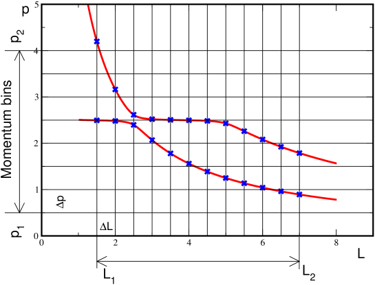
Figure 1: Schematic plot describing the construction of the probability distribution from the energy levels.

• Choose the first $N$ energy levels (e.g., $N=2$ in Fig. 1); choose the interval $L\in[L_{1},L_{2}]$ and slice this interval into equal parts with length $\Delta L$. For each value of $L=L_{1}$, $L=L+\Delta L$, etc determine $p_{n}(L),~{}n=1\cdots N$.

• Choose a corresponding momentum interval $p\in[p_{1},p_{2}]$ and introduce equal-size momentum bins with length $\Delta p$.

• Count, how many times the eigenvalue $p_{n}(L),~{}n=1\cdots N$ is contained in a particular bin, if $L$ runs from $L_{1}$ to $L_{2}$. This number gives the unnormalized probability distribution for the momentum bin chosen. Normalizing this distribution in the interval $[p_{1},p_{2}]$ yields finally the probability distribution $W(p)$ we are looking for. The normalization condition is given by

  $$\sum_{k=0}^{M_{P}}W(p_{1}+k\Delta p)\Delta p=1\,,\quad M_{P}=\frac{p_{2}-p_{1}}{\Delta p}-1\,.$$ (34)

It is clear that in case of a pronounced avoided level crossing, the probability distribution $W(p)$ must be strongly peaked around the resonance energy. The exact shape of $W(p)$ can be predicted on the basis of Lüscher’s formula. To this end, note that, in the limit of infinitesimally small $L-$ and $p-\,$bins, $W(p)$ is given by

$$W(p)=C\sum_{n=1}^{N}\frac{1}{p^{\prime}_{n}(L)}\,,$$ (35)

where $C$ is a normalization constant.

For simplicity, we consider here the scattering in the partial wave with $L=1,~{}J=\frac{3}{2}$ and neglect the (small) mixing to higher partial waves. Using table 1 and Eq. (32), the relation between the finite-volume energy spectrum and the phase shift $\delta(p)$ takes the form

$$\delta(p)=-\phi(\kappa)+\pi n,\quad\quad\phi(\kappa)=-\arctan\frac{\pi^{3/2}\kappa}{Z_{00}(1;\kappa^{2})}\,,\quad\quad\kappa=\frac{pL}{2\pi}\,,$$ (36)

where the integer $n$ labels the energy levels $p_{n}(L)$, which are the solutions of the above equation.

Differentiating now Eq. (36) with respect to $L$ and substituting into Eq. (35), we obtain

$$W(p)=C\sum_{n=1}^{N}\left(\frac{L_{n}(p)}{p}+\frac{2\pi\delta^{\prime}(p)}{p\phi^{\prime}(\kappa_{n}(p))}\right)\,.$$ (37)

where $\kappa_{n}(p)$ and $L_{n}(p)$ are the solutions of Eq. (36) for a given $p$. It is seen that $W(p)$ defined by Eq. (37) is closely related to the so-called “density of states in a finite volume,” see e.g. Ref. [46].

In the vicinity of the resonance, $\delta^{\prime}(p)$ is strongly peaked. Substituting a Breit-Wigner parameterization for $\delta(p)$ and assuming that all other factors smoothly depend on the momentum $p$, we may verify that in the vicinity of the resonance the function $W(p)$ follows the Breit-Wigner form for the scattering cross section, with the same width.

A useful parameterization of $W(p)$ can be obtained by using the following approximation of the function $\phi(\kappa)$, which is valid in a large interval of arguments [20]

$$\phi(\kappa)=\pi c\kappa^{2}\,,\qquad c\simeq 1\,.$$ (38)

Solving Lüscher’s equation, we obtain

$$L_{n}(p)=\frac{1}{p}\sqrt{4\pi(\pi n-\delta(p))}$$ (39)

and

$$W(p)=\frac{C}{p}\,\sum_{n=1}^{N}\biggl{(}\frac{\sqrt{4\pi(\pi n-\delta(p))}}{p}+\frac{2\pi\delta^{\prime}(p)}{\sqrt{4\pi(\pi n-\delta(p))}}\biggr{)}\,.$$ (40)

In order to suppress the (large) background, related to the free motion of the $\pi N$ pair, we consider in the following the so-called subtracted probability distribution $W(p)-W_{0}(p)$, where $W_{0}(p)$ is determined from Eq. (37) with $\delta(p)=0$ and $L_{n}(p)$ corresponding to the free energy levels.

It is interesting to consider the infinite-volume limit of the probability distribution. Note that in this limit the number of energy levels per fixed momentum bin goes to infinity. Consequently, the number of levels $N$ in Eq. (36) can be chosen very large. In this case, in the expression for the quantity $L_{n}(p)$ which is determined through the solution of Lüscher’s equation

$$L_{n}(p)=\frac{2\pi}{p}\phi^{-1}\left(\pi n-\delta(p)\right)\,,$$ (41)

the phase shift obeys the inequality $\delta(p)\ll\pi n$ for the large majority of terms in the sum over energy levels. Expanding in a Taylor series, we get

$$L_{n}(p)=\frac{2\pi}{p}\,\bar{\kappa}_{n}-\frac{2\pi}{p}\delta(p)\frac{1}{\phi^{\prime}(\bar{\kappa}_{n})}+O(\delta^{2})~{},$$ (42)

with $\bar{\kappa}_{n}$ is the solution of the equation $\phi(\bar{\kappa}_{n})=\pi n$. Using, in addition, $\kappa_{n}=\bar{\kappa}_{n}+O(\delta)$, the unnormalized probability distribution for $N\to\infty$ takes the form

$$C^{-1}W(p)=\frac{2\pi}{p^{2}}\sum_{n=1}^{N}\bar{\kappa}_{n}+\frac{2\pi}{p}\sum_{n=1}^{N}\frac{1}{\phi^{\prime}(\bar{\kappa}_{n})}\left(\frac{\delta(p)}{p}-\delta^{\prime}(p)\right)+O(\delta^{2})~{}.$$ (43)

The first term exactly coincides with the free background. Subtracting this background and taking into account the fact that the quantity $\sum_{n=1}^{N}(\phi^{\prime}(\bar{\kappa}_{n}))^{-1}$ does not depend on the phase $\delta(p)$, we obtain

$$C^{-1}W(p)-C_{0}^{-1}W_{0}(p)\propto\frac{1}{p}\left(\frac{\delta(p)}{p}-\delta^{\prime}(p)\right)\,.$$ (44)

In other words, in the infinite-volume limit this quantity is determined by the elastic phase shift alone.

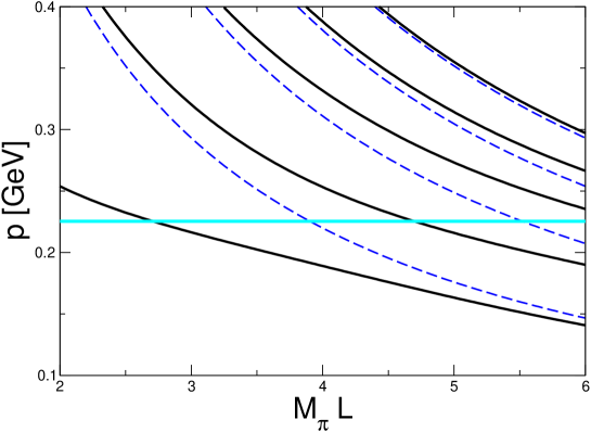
Figure 2: Volume dependence of the spectrum of the Hamiltonian (solid lines), predicted by using Lüscher’s formula with input experimental $P_{33}$ phase shift. The center-of-mass momentum $p$ vs the box size $L$ is shown. For comparison, the free energy levels for the $\pi N$ system are given (dashed lines). The horizontal line marks the position of the $\Delta$ resonance. It is seen that the avoided level crossing is completely washed out.

5 Analysis of synthetic data

In this section we will implement the method discussed in the previous section for analyzing data. In the absence of lattice QCD data we will use synthetic data on the spectrum of the Hamiltonian, which are produced by using experimentally measured phase shifts [47] in Lüscher’s formula. If in the future unquenched lattice calculations are performed at the physical quark masses, the results must agree with the above synthetic data set.

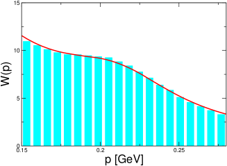
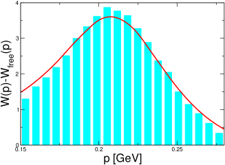
Figure 3: Unsubtracted (left panel) and subtracted (right panel) probability distributions. Only the lowest energy level has been included in the analysis ($N=1$). The solid lines correspond to the prediction made by using Lüscher’s formula with an approximation $\phi(\kappa)\simeq\pi\kappa^{2}$ (see the text for details). A clear resonance-like structure is observed in the subtracted distribution.

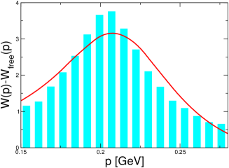
Figure 4: The same as in Fig. 3 but obtained only from 5 data points corresponding to $M_{\pi}L=1.4,~{}2.55,~{}3.7,~{}4.85,~{}6$. The values of the function $p(L)$ between the data points are obtained using Spline interpolation. Only the lowest energy level is analyzed ($N=1$). The interval in the variable $p$ is the same as in Fig. 3. It is seen that 5 data points do not provide a very good accuracy over this interval in $L$: the subtracted probability distribution is rather different from the theoretical prediction made on the basis of Lüscher’s formula.

The calculated spectrum, obtained by substituting the resonant $P_{33}$ partial wave phase shift into Lüscher’s formula, is shown in Fig. 2. In this figure, the relative momentum of the $\pi N$ system $p(L)$, corresponding to the discrete energy levels of the Hamiltonian in a finite box, is plotted against the box size $L$ (in units of $M_{\pi}^{-1}$). It is seen that the structure of the energy levels is smooth: the avoided level crossing has been completely washed out due to the relatively large width of $\Delta$. However, in the same figure we also plot the free energy levels, demonstrating that in the vicinity of the resonance a continuous rearrangement of the spectrum takes place.

This rearrangement can be made explicitly visible by performing the analysis of the energy spectrum, using the probability distribution method introduced above. Constructing, as described above, the unsubtracted probability distribution $W(p)$ from the lowest energy level yields the plot shown on the left panel of Fig. 3. The resonance is seen as a barely distinguishable shoulder around $p\simeq 0.22~{}\mbox{GeV}$. This result, which obviously reflects the washing-out of the avoided level crossing in Fig. 2, casts justified doubts on the feasibility of a clean extraction of the $\Delta$-resonance parameters from the data. The picture, however, completely changes once the subtraction of the background due to free $\pi N$ pairs has been performed, see the right panel in Fig. 3. The resonance-like structure in the subtracted distribution is clearly visible, allowing one to finally conclude that the determination of the resonance parameters from the data is indeed possible. On both plots the solid curves correspond to the theoretical prediction made on the basis of Lüscher’s formula. In order to simplify the numerical calculations, the curves were constructed by using the approximation $\phi(\kappa)\simeq\pi\kappa^{2}$, which works very well for all relevant values of the variable $\kappa$. Since these curves are shown for the demonstrative purposes only, a better accuracy is not needed here.

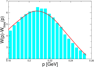
Figure 5: The subtracted probability distribution for 10 data points equally distributed in the interval $M_{\pi}L=1.4\cdots 6$ (left panel). The same with 5 data points, $M_{\pi}L=1.9\cdots 4.5$ (right panel). In both cases, only the lowest energy level has been included in the analysis ($N=1$). The agreement with the theoretical curve, based on Lüscher’s formula, is much better than for Fig. 4 (right panel).

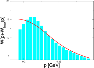
Figure 6: A non-uniform choice of the data points $M_{\pi}L=1.4,~{}1.6,~{}1.8,~{}2.8,~{}3.9$. The momentum interval is chosen to be $p\in[0.21,0.35]~{}\mbox{GeV}$. It is immediately seen that the subtracted probability distribution deviates from the theoretically predicted behavior in the interval where the data points are sparse (large volumes or small momenta).

Up to now, we have dealt with the exact solution of Lüscher’s equation for the energy spectrum that on the lattice corresponds to measuring this spectrum at infinite accuracy and at all values of $L$. The situation in real calculations is different. Here one expects to get at most a few data points for different volumes. Our next aim is to mimic this situation in the calculations with the synthetic data and check whether the extraction of the resonance parameters is still possible. The probability distribution method, which we are using, is equivalent to Lüscher’s approach and provides just a nice tool to visualize the final result.

In order to achieve the goal formulated above, we first perform the analysis in the same momentum interval as in Fig. 3, but using 5 uniformly distributed data points, located at $M_{\pi}L=1.4,~{}2.55,~{}3.7,~{}4.85,~{}6$. The values of $p(L)$ between these data points were reconstructed by using the interpolation procedure with cubic splines. The result for the unsubtracted and subtracted probability distributions is shown in Fig. 4. It is clear that providing only 5 data points at this quite large interval of the variable $L$ does not ensure a very high accuracy: the shape of the resonance comes out distorted. Moreover, one might expect that if even less data points are included in the analysis (see, e.g. [37]), the determined resonance parameters will include large systematic uncertainty which is very hard to control.

There can be two possible ways out. One may try to gradually increase the number of data points, or one may try to reduce the size of the momentum and volume interval just to an immediate proximity of the resonance. Both possibilities have been tried, as shown in Fig. 5. The left panel of this figure corresponds to using 10 data points instead of 5 in the same interval, whereas the right panel corresponds to reducing the interval to $M_{\pi}L\in[1.9,4.5]$, respectively. In both cases one observes a clear improvement as compared to the case shown in Fig. 4. Note also that the data points should not not be uniformly distributed in $L$, but have indeed to be concentrated on both sides of the resonance. Otherwise, one may arrive to the picture shown in Fig. 6, where we show the probability distribution, obtained from the following data points: $M_{\pi}L=1.4,~{}1.6,~{}1.8,~{}2.8,~{}3.9$. It is seen that the probability distribution significantly deviates from the exact theoretical prediction in that part of the interval, where the data points are sparse.

Finally, we have applied the method of probability distributions to the simultaneous analysis of the first two energy levels. The figure 7 contains the information about 10 data points, uniformly distributed in the interval $M_{\pi}L\in[2,6.5]$. The resulting resonance shape is again in good agreement with the theoretical prediction, made on the basis of Lüscher’s formula. Note that the resonance parameters extracted from the analysis of the different energy levels must of course coincide. In case the data from the excited levels are also available, checking the stability of the resonance parameters might enable one to verify a posteriori, whether the volumes, used in the calculation, are large enough to justify the application of Lüscher’s approach.

Last but not least, the lattice data on the measured spectrum always come with errors. Our method provides an easy tool to render the analysis transparent in this case as well. The procedure is described below.

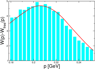
Figure 7: The result of the analysis of the lowest two energy levels ($N=2$) with 10 data points, $M_{\pi}L=2\cdots 6.5$. The resonance structure reasonably reproduces the theoretical prediction on the basis of Lüscher’s formula.

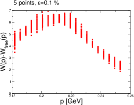
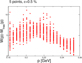
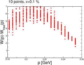
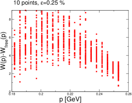
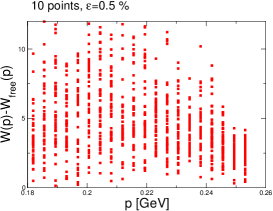
Figure 8: Probability distributions, obtained from the data that contain errors (see the text for the details). The central data points are the same as in Fig. 5. As seen from the figure, the resonance structure is effectively washed out already at a relative error of $0.5\%$ in the data or even earlier.

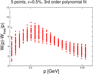
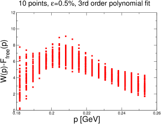
Figure 9: The same as in Fig. 8 at a relative error $\varepsilon=0.5\%$. A polynomial fit to the random data was used prior to producing the probability distribution. The improvement as compared to Fig. 8 is clearly visible. The peak is washed out approximately at $\varepsilon\simeq 0.75\%\cdots 1\%$.

We start from the data equidistantly distributed in the interval $M_{\pi}L\in[1.9,4.5]$ (5 or 10 data points, as in Fig. 8). From each data point $E_{i}=E(L_{i})$ we further produce a statistical sample of 50 data points at a same $L_{i}$, which are normally distributed around the central value $E_{i}$ with the standard deviation $\sigma_{i}=\varepsilon E_{i}$. The figure 8 shows the probability distributions obtained from these randomly produced data, for three different values of $\varepsilon=0.1\%,0.25\%,0.5\%$. Spline interpolation is used between data points. It is evident that the nice resonance structure, which was seen in the probability distribution (data with no errors), is washed out already at quite small values of the relative error assigned. Interestingly enough, the increase of the number of data points does not lead to an improved accuracy. The reason for this is that we treat the neighboring data points to be statistically independent. If the distance between the neighboring points is decreased, the fluctuations in the derivative of the eigenvalues increase and this leads to the increase of the statistical noise in the probability distribution (see Fig. 8).

These statistical fluctuations can be suppressed to some extent if we perform a smooth (e.g. polynomial) interpolation of random data prior to calculation of the probability distribution. This is demonstrated in Fig. 9 where the random data on the spectrum were first fitted as $p(L)=a_{0}+a_{1}L+a_{2}L^{2}+a_{3}L^{3}$ prior to producing the probability distribution. The situation clearly improves, especially in the case of 10 data points. Still, from Figs. 8 and 9 one has to conclude that a very accurate measurement of the spectrum is indeed needed to reliably extract the properties of the $\Delta$-resonance.

6 Conclusions

• Within the covariant non-relativistic effective field theory [43] we have derived Lüscher’s formula for scattering of spin-1/2 and spin-$0$ particles. The partial-wave expansion is performed, and the cubic symmetry on the lattice is used to reduce the resulting matrix equations.

• The notion of probability distribution for the finite-volume spectrum of the Hamiltonian is introduced. It is shown that near the resonance energy the probability distribution behaves similar to the scattering cross section in the infinite volume: it produces a Breit-Wigner peak at the resonance energy with the same width.

• The probability distribution, which is directly constructed from the energy levels, does not contain any prior bias. For this reason, the analysis carried out with the use of this method can be used to judge whether a clean extraction of the resonance parameters from the available data is possible.

• The probability distribution does not carry more or less physical information than Lüscher’s formula. The advantage of the probability distribution is its visual transparency. The choice of the method in the actual analysis is dictated by convenience.

• In the present paper we apply the method of probability distribution to the case of the $\Delta$-resonance. We observe that the distribution after subtracting the background corresponding to the free motion of the $\pi N$ pair develops a nice resonance structure in accordance with the exact prediction based on Lüscher’s formula – even though the avoided level crossing is completely washed out.

• It is possible to achieve a satisfactory description of the resonance position and shape even with few data points, provided they are chosen close enough to the resonance and are measured very accurately. Measurement of only the ground state suffices (inclusion of the excited levels provides additional check on the results). To conclude, the results of the paper clearly demonstrate that the extraction of the resonance parameters from the measurement of the finite-volume energy spectrum by using Lüscher’s method is indeed a feasible although difficult task.

Acknowledgments

We are grateful to J. Gasser, H. Krebs, J. Negele, F. Niedermayer, H. Petry, G. Schierholz, U.-J. Wiese and U. Wenger for useful discussions.

Appendix A Basis vectors of the cubic group

In this appendix we collect the basic formulae for the representations of the cubic group, which are needed for partial diagonalization of Lüscher’s formula.

Consider first shortly the case without spin. The group $O$ of the symmetries of the 3-dimensional cube has 24 elements (no reflections included), which fall into 5 conjugacy classes: $I$ (identity), $3C_{2}$, $8C_{3}$, $6C_{4}$ and $6C_{2}^{\prime}$ (see, e.g. [45, 48]). We find it convenient to parametrize the group elements by specifying three Euler angles $\alpha,\beta,\gamma$. Alternatively, the element can be parametrized, e.g., by specifying the axis ${\bf n}$ and the rotation angle $\omega$. The table A.1 collects the values of the group parameters.

Class	$i$	${\bf n}$	$\omega$	$\alpha$	$\beta$	$\gamma$
$I$	1	any	$0$	$0$	$0$	$0$
$8C_{3}$	2	$(1,1,1)$	$-2\pi/3$	$-\pi/2$	$-\pi/2$	$0$
	3	$(1,1,1)$	$2\pi/3$	$0$	$\pi/2$	$\pi/2$
	4	$(-1,1,1)$	$-2\pi/3$	$0$	$-\pi/2$	$-\pi/2$
	5	$(-1,1,1)$	$2\pi/3$	$\pi/2$	$\pi/2$	$0$
	6	$(-1,-1,1)$	$-2\pi/3$	$-\pi/2$	$\pi/2$	$0$
	7	$(-1,-1,1)$	$2\pi/3$	$0$	$-\pi/2$	$\pi/2$
	8	$(1,-1,1)$	$-2\pi/3$	$0$	$\pi/2$	$-\pi/2$
	9	$(1,-1,1)$	$2\pi/3$	$\pi/2$	$-\pi/2$	$0$
$6C_{4}$	10	$(1,0,0)$	$-\pi/2$	$-\pi/2$	$-\pi/2$	$\pi/2$
	11	$(1,0,0)$	$\pi/2$	$\pi/2$	$-\pi/2$	$-\pi/2$
	12	$(0,1,0)$	$-\pi/2$	$0$	$-\pi/2$	$0$
	13	$(0,1,0)$	$\pi/2$	$0$	$\pi/2$	$0$
	14	$(0,0,1)$	$-\pi/2$	$-\pi/2$	$0$	$0$
	15	$(0,0,1)$	$\pi/2$	$\pi/2$	$0$	$0$
$6C^{\prime}_{2}$	16	$(0,1,1)$	$-\pi$	$-\pi/2$	$-\pi/2$	$-\pi/2$
	17	$(0,-1,1)$	$-\pi$	$-\pi/2$	$\pi/2$	$-\pi/2$
	18	$(1,1,0)$	$-\pi$	$-\pi/2$	$-\pi$	$0$
	19	$(1,-1,0)$	$-\pi$	$0$	$\pi$	$-\pi/2$
	20	$(1,0,1)$	$-\pi$	$0$	$\pi/2$	$-\pi$
	21	$(-1,0,1)$	$-\pi$	$0$	$-\pi/2$	$-\pi$
$3C_{2}$	22	$(1,0,0)$	$-\pi$	$\pi$	$\pi$	$0$
	23	$(0,1,0)$	$-\pi$	$0$	$-\pi$	$0$
	24	$(0,0,1)$	$-\pi$	$0$	$0$	$-\pi$

Table A.1: Parameterization of the elements of cubic group. The vector ${\bf n}$ should be normalized to unity.

The irreducible representations of the rotation group $D^{L}$, $L=0,1,\cdots$ are defined in the $2L+1$-dimensional space spanned on the basis vectors $|LM\rangle$. These representations are reducible under the cubic group $O$ and can be decomposed into the irreducible representations of the latter denoted by $\Gamma=A_{1},A_{2},E,T_{1}~{}\mbox{and}~{}T_{2}$. The dimension of these representations $N(\Gamma)$ is equal to 1,1,2,3,3, respectively.

In order to construct the basis of the irreducible representations, we consider the linear operator $P_{\alpha\beta}^{\Gamma,L}$, whose matrix elements in the space spanned by the vectors $|LM\rangle$ are given by

$$(P_{\alpha\beta}^{\Gamma,L})_{MM^{\prime}}=\sum_{i=1}^{24}(R_{i}^{\Gamma})^{*}_{\alpha\beta}\,D^{L}_{MM^{\prime}}(\alpha_{i},\beta_{i},\gamma_{i})\,,$$ (A.1)

where $D^{L}_{MM^{\prime}}(\alpha_{i},\beta_{i},\gamma_{i})$ are Wigner $D$-functions, and $(R_{i}^{\Gamma})_{\alpha\beta}$, $\alpha,\beta=1\cdots N(\Gamma)$ denote the matrices of the irreducible representations of cubic group

• $A_{1}$ is the trivial 1-dimensional representation $R_{i}=1$.

• $R_{i}=-1$ for the conjugacy classes $6C_{4}$ and $6C_{2}^{\prime}$, $R_{i}=1$ otherwise.

• The matrices in this representation are two-dimensional and real:

  $$R_{i} = {\bf 1}\quad\mbox{for}\quad i=1,22,23,24,$$

  $$R_{i} = \sigma_{3}\quad\mbox{for}\quad i=14,15,18,19,$$

  $$R_{i} = -\cos\frac{\pi}{3}\,{\bf 1}+i\sin\frac{\pi}{3}\,\sigma_{2}\quad\mbox{for}\quad i=2,5,6,9,$$

  $$R_{i} = -\cos\frac{\pi}{3}\,{\bf 1}-i\sin\frac{\pi}{3}\,\sigma_{2}\quad\mbox{for}\quad i=3,4,7,8,$$

  $$R_{i} = -\cos\frac{\pi}{3}\,\sigma_{3}-\sin\frac{\pi}{3}\,\sigma_{1}\quad\mbox{for}\quad i=10,11,16,17,$$

  $$R_{i} = -\cos\frac{\pi}{3}\,\sigma_{3}+\sin\frac{\pi}{3}\,\sigma_{1}\quad\mbox{for}\quad i=12,13,20,21.$$ (A.2)

• $(R_{i})_{\alpha\beta}=\exp\biggl{(}-i{\bf n}^{(i)}{\bf J}\,\omega_{i}\biggr{)}_{\alpha\beta}=\cos\omega_{i}\delta_{\alpha\beta}+(1-\cos\omega_{i})n_{\alpha}^{(i)}n_{\beta}^{(i)}-\sin\omega_{i}\varepsilon_{\alpha\beta\gamma}n_{\gamma}^{(i)}$, where $(J_{\gamma})_{\alpha\beta}=-i\varepsilon_{\alpha\beta\gamma}$ denote the group generators.

• The matrices are the same as in the irreducible representation $T_{1}$, except the change of sign for the conjugacy classes $6C_{4}$ and $6C_{2}^{\prime}$.

The basis vectors of the irreducible representations are obtained by acting with the linear operator given by Eq. (A.1) at a fixed $\beta$ and varying $\alpha$ on an arbitrary vector $\phi_{M}$ from the space spanned by the vectors $|LM\rangle$

$$(e_{\alpha}^{\Gamma,L,\beta})_{M}={\cal N}\,\sum_{M^{\prime}=-L}^{L}(P_{\alpha\beta}^{\Gamma,L})_{MM^{\prime}}\phi_{M^{\prime}}\,,\quad\quad\alpha=1\cdots N_{\Gamma}\,,\quad\quad\beta~{}\mbox{fixed}\,,$$ (A.3)

where ${\cal N}$ denotes the normalization constant. It is fixed so that the basis vectors obey the orthonormality condition

$$\sum_{M}(e_{\alpha^{\prime}}^{\Gamma^{\prime},L,\beta})^{*}_{M}\,(e_{\alpha}^{\Gamma,L,\beta})_{M}=\delta_{\alpha^{\prime}\alpha}\delta_{\Gamma^{\prime}\Gamma}\,.$$ (A.4)

If the representation $\Gamma$ is not contained in $D^{L}$, the action of the projection operator on $\phi_{M}$ gives 0. The equations (A.3) and (A.4) do not fix a common phase of the basis vectors, belonging to the same representation labeled with $L,\Gamma$ – this can be freely chosen. If a representation $\Gamma$ enters more than once in $D^{L}$, an additional orthogonalization of the basis vectors, belonging to the same representation, is necessary. Inclusion of parity is trivial. The basis vectors are simultaneously the eigenvectors of $S_{2}$ with the eigenvalue $P=(-)^{L}$.

In table A.2 we list the basis vectors of the irreducible representations of the cubic group up to $L=4$, obtained from Eq. (A.3). The phases are chosen so that after the partial diagonalization of Lüscher’s equation, the entries of table E.2 in Ref. [19] are reproduced.

Note also that our basis differs from the one given in Ref. [49] and can not be reduced to it with a single unitary transformation for all $L$. We have also checked that the use of the basis from Ref. [49] does not lead to Eq. (31): e.g., the different irreducible representations turn out not to be orthogonal.

Our basis vectors can be transformed into those listed in Ref. [50] by unitary transformations. Since in that article the basis vectors of the same irreducible representation, belonging to different values of $L$, are not fully displayed, we can not carry out this comparison to the end.

$\Gamma$	$L$	$\alpha$	Basis vectors
$A_{1}^{+}$	$0$	1	$|0,0\rangle$
$T_{1}^{-}$	$1$	1	$\frac{1}{\sqrt{2}}\,(|1,-1\rangle-|1,1\rangle)$
		2	$\frac{i}{\sqrt{2}}\,(|1,-1\rangle+|1,1\rangle)$
		3	$|1,0\rangle$
$T_{2}^{+}$	$2$	1	$-\frac{1}{\sqrt{2}}\,(|2,-1\rangle+|2,1\rangle)$
		2	$\frac{i}{\sqrt{2}}\,(|2,-1\rangle-|2,1\rangle)$
		3	$-\frac{1}{\sqrt{2}}\,(|2,-2\rangle-|2,2\rangle)$
$E^{+}$	$2$	1	$|2,0\rangle$
		2	$\frac{1}{\sqrt{2}}\,(|2,-2\rangle+|2,2\rangle)$
$T_{1}^{-}$	$3$	1	$\frac{\sqrt{5}}{4}\,(|3,-3\rangle-|3,3\rangle)-\frac{\sqrt{3}}{4}\,(|3,-1\rangle-|3,1\rangle)$
		2	$\frac{-i\sqrt{5}}{4}\,(|3,-3\rangle+|3,3\rangle)-\frac{i\sqrt{3}}{4}\,(|3,-1\rangle+|3,1\rangle)$
		3	$|3,0\rangle$
$T_{2}^{-}$	$3$	1	$-\frac{\sqrt{3}}{4}\,(|3,-3\rangle-|3,3\rangle)-\frac{\sqrt{5}}{4}\,(|3,-1\rangle-|3,1\rangle)$
		2	$\frac{-i\sqrt{3}}{4}\,(|3,-3\rangle+|3,3\rangle)+\frac{i\sqrt{5}}{4}\,(|3,-1\rangle+|3,1\rangle)$
		3	$\frac{1}{\sqrt{2}}\,(|3,-2\rangle+|3,2\rangle)$
$A_{2}^{-}$	$3$	1	$\frac{1}{\sqrt{2}}\,(|3,-2\rangle-|3,2\rangle)$
$T_{1}^{+}$	$4$	1	$-\frac{1}{4}\,(|4,-3\rangle+|4,3\rangle)-\frac{\sqrt{7}}{4}\,(|4,-1\rangle+|4,1\rangle)$
		2	$\frac{i}{4}\,(|4,-3\rangle-|4,3\rangle)-\frac{i\sqrt{7}}{4}\,(|4,-1\rangle-|4,1\rangle)$
		3	$\frac{1}{\sqrt{2}}\,(|4,-4\rangle-|4,4\rangle)$
$T_{2}^{+}$	$4$	1	$\frac{\sqrt{7}}{4}\,(|4,-3\rangle+|4,3\rangle)-\frac{1}{4}\,(|4,-1\rangle+|4,1\rangle)$
		2	$\frac{i\sqrt{7}}{4}\,(|4,-3\rangle-|4,3\rangle)+\frac{i}{4}\,(|4,-1\rangle-|4,1\rangle)$
		3	$\frac{1}{\sqrt{2}}\,(|4,-2\rangle-|4,2\rangle)$
$E^{+}$	$4$	1	$-\frac{\sqrt{42}}{12}\,(|4,-4\rangle+|4,4\rangle)+\frac{\sqrt{15}}{6}\,|4,0\rangle$
		2	$-\frac{1}{\sqrt{2}}\,(|4,-2\rangle+|4,2\rangle)$
$A_{1}^{+}$	$4$	1	$\frac{\sqrt{30}}{12}\,(|4,-4\rangle+|4,4\rangle)+\frac{\sqrt{21}}{6}\,|4,0\rangle$

Table A.2: The normalized basis of the irreducible representations of the cubic group: integer values of the angular momentum.

In order to include the particles with spin, one has to consider the double cover of $O$ denoted by ${}^{2}O$, which can be constructed by adding a negative identity for $\pm 2\pi$ rotations to the group $O$ [45]. One ends up with a group of 48 elements divided into 8 conjugacy classes (see table A.3) and, accordingly, with 8 irreducible representations. In addition to the previously considered 5, one has 3 new representations denotes as $\Gamma=G_{1},G_{2},H$ with the dimension $N(\Gamma)=2,2,4$, respectively. In case of the half-integer total momentum $J$, one needs to consider only these additional even-dimensional representations.

Class	$i$	${\bf n}$	$\omega$	Class	$i$	${\bf n}$	$\omega$
$I$	1	any	$0$	$8C_{3}$	28	$(1,1,1)$	$4\pi/3$
$6C_{4}$	2	$(1,0,0)$	$\pi$		29	$(-1,1,1)$	$4\pi/3$
	3	$(0,1,0)$	$\pi$		30	$(-1,-1,1)$	$4\pi/3$
	4	$(0,0,1)$	$\pi$		31	$(1,-1,1)$	$4\pi/3$
	5	$(1,0,0)$	$-\pi$		32	$(1,1,1)$	$-4\pi/3$
	6	$(0,1,0)$	$-\pi$		33	$(-1,1,1)$	$-4\pi/3$
	7	$(0,0,1)$	$-\pi$		34	$(-1,-1,1)$	$-4\pi/3$
$6C^{\prime}_{8}$	8	$(1,0,0)$	$\pi/2$		35	$(1,-1,1)$	$-4\pi/3$
	9	$(0,1,0)$	$\pi/2$	$12C^{\prime}_{4}$	36	$(0,1,1)$	$\pi$
	10	$(0,0,1)$	$\pi/2$		37	$(0,-1,1)$	$\pi$
	11	$(1,0,0)$	$-\pi/2$		38	$(1,1,0)$	$\pi$
	12	$(0,1,0)$	$-\pi/2$		39	$(1,-1,0)$	$\pi$
	13	$(0,0,1)$	$-\pi/2$		40	$(1,0,1)$	$\pi$
$6C_{8}$	14	$(1,0,0)$	$3\pi/2$		41	$(-1,0,1)$	$\pi$
	15	$(0,1,0)$	$3\pi/2$		42	$(0,1,1)$	$-\pi$
	16	$(0,0,1)$	$3\pi/2$		43	$(0,-1,1)$	$-\pi$
	17	$(1,0,0)$	$-3\pi/2$		44	$(1,1,0)$	$-\pi$
	18	$(0,1,0)$	$-3\pi/2$		45	$(1,-1,0)$	$-\pi$
	19	$(0,0,1)$	$-3\pi/2$		46	$(1,0,1)$	$-\pi$
$8C_{6}$	20	$(1,1,1)$	$2\pi/3$		47	$(-1,0,1)$	$-\pi$
	21	$(-1,1,1)$	$2\pi/3$	$J$	48	any	$2\pi$
	22	$(-1,-1,1)$	$2\pi/3$
	23	$(1,-1,1)$	$2\pi/3$
	24	$(1,1,1)$	$-2\pi/3$
	25	$(-1,1,1)$	$-2\pi/3$
	26	$(-1,-1,1)$	$-2\pi/3$
	27	$(1,-1,1)$	$-2\pi/3$

Table A.3: Parameterization of the elements of the double cover of the cubic group. The vector ${\bf n}$ should be normalized to unity.

The matrices of the irreducible representations $G_{1},G_{2},H$ are given by [45]

• $(R_{i})_{\alpha\beta}=\exp\biggl{(}-\frac{i}{2}\,{\bf n}^{(i)}\mbox{\boldmath$\sigma$}\,\omega_{i}\biggr{)}_{\alpha\beta}=\delta_{\alpha\beta}\cos\frac{\omega_{i}}{2}-i{\bf n}^{(i)}\mbox{\boldmath$\sigma$}_{\alpha\beta}\sin\frac{\omega_{i}}{2}$.

• the matrices are the same except change the sign in the conjugacy classes $6C_{8},6C_{8}^{\prime}$ and $12C_{4}^{\prime}$.

• the matrices $(R_{i})_{\alpha\beta}=\exp\biggl{(}-i{\bf n}^{(i)}{\bf J}^{\frac{3}{2}}\,\omega_{i}\biggr{)}_{\alpha\beta}$ where ${\bf J}^{\frac{3}{2}}_{\alpha\beta}$ denote the group generators in spin-3/2 case.

The counterpart of Eq. (A.1) in case of the half-integer total momentum $J$ is

$$(P_{\alpha\beta}^{\Gamma,J})_{MM^{\prime}}=\sum_{i=1}^{48}(R_{i}^{\Gamma})^{*}_{\alpha\beta}\,D^{J}_{MM^{\prime}}(\alpha_{i},\beta_{i},\gamma_{i})\,.$$ (A.5)

Acting with the linear operator $P_{\alpha\beta}^{\Gamma,J}$ on an arbitrary linear combination of the basis vectors $|JM\rangle^{\pm}$ defined in section 3, we obtain the basis of the irreducible representations $G_{1},G_{2}$ and $H$. Inclusion of parity is again trivial, since the basis vectors $|JM\rangle^{\pm}$ are the eigenvectors of parity, with the eigenvalue $P=\pm 1=(-)^{L}$. Up to the value $J=\frac{7}{2}$, these basis vectors are listed in table A.4

$\Gamma^{\pm}$	$J$	$\alpha$	Basis vectors
$G1^{\pm}$	$1/2$	1	$|\frac{1}{2}~{}\frac{1}{2}\rangle^{\pm}$
		2	$|\frac{1}{2}~{}-\frac{1}{2}\rangle^{\pm}$
$G1^{\pm}$	$7/2$	1	$\frac{\sqrt{15}}{6}\,|\frac{7}{2}~{}-\frac{7}{2}\rangle^{\pm}+\frac{\sqrt{21}}{6}\,|\frac{7}{2}~{}\frac{1}{2}\rangle^{\pm}$
		2	$\frac{-\sqrt{21}}{6}\,|\frac{7}{2}~{}-\frac{1}{2}\rangle^{\pm}\par-\frac{\sqrt{15}}{6}\,|\frac{7}{2}~{}\frac{7}{2}\rangle^{\pm}$
$G2^{\pm}$	$5/2$	1	$\frac{\sqrt{30}}{6}\,|\frac{5}{2}~{}-\frac{3}{2}\rangle^{\pm}-\frac{\sqrt{6}}{6}\,|\frac{5}{2}~{}\frac{5}{2}\rangle^{\pm}$
		2	$-\frac{\sqrt{6}}{6}\,|\frac{5}{2}~{}-\frac{5}{2}\rangle^{\pm}+\frac{\sqrt{30}}{6}\,|\frac{5}{2}~{}\frac{3}{2}\rangle^{\pm}$
$G2^{\pm}$	$7/2$	1	$-\frac{1}{2}\,|\frac{7}{2}~{}-\frac{3}{2}\rangle^{\pm}+\frac{\sqrt{3}}{2}\,|\frac{7}{2}~{}\frac{5}{2}\rangle^{\pm}$
		2	$-\frac{\sqrt{3}}{2}\,|\frac{7}{2}~{}-\frac{5}{2}\rangle^{\pm}+\frac{1}{2}\,|\frac{7}{2}~{}\frac{3}{2}\rangle^{\pm}$
$H^{\pm}$	$3/2$	1	$|\frac{3}{2}~{}\frac{3}{2}\rangle^{\pm}$
		2	$|\frac{3}{2}~{}\frac{1}{2}\rangle^{\pm}$
		3	$|\frac{3}{2}~{}-\frac{1}{2}\rangle^{\pm}$
		4	$|\frac{3}{2}~{}-\frac{3}{2}\rangle^{\pm}$
$H^{\pm}$	$5/2$	1	$\frac{-\sqrt{30}}{6}\,|\frac{5}{2}~{}-\frac{5}{2}\rangle^{\pm}-\frac{\sqrt{6}}{6}\,|\frac{5}{2}~{}\frac{3}{2}\rangle^{\pm}$
		2	$|\frac{5}{2}~{}\frac{1}{2}\rangle^{\pm}$
		3	$-~{}|\frac{5}{2}~{}-\frac{1}{2}\rangle^{\pm}$
		4	$\frac{\sqrt{6}}{6}\,|\frac{5}{2}~{}-\frac{3}{2}\rangle^{\pm}+\frac{\sqrt{30}}{6}\,|\frac{5}{2}~{}\frac{5}{2}\rangle^{\pm}$
$H^{\pm}$	$7/2$	1	$\frac{1}{2}\,|\frac{7}{2}~{}-\frac{5}{2}\rangle^{\pm}+\frac{\sqrt{3}}{2}\,|\frac{7}{2}~{}\frac{3}{2}\rangle^{\pm}$
		2	$\frac{\sqrt{21}}{6}\,|\frac{7}{2}~{}-\frac{7}{2}\rangle^{\pm}-\frac{\sqrt{15}}{6}\,|\frac{7}{2}~{}\frac{1}{2}\rangle^{\pm}$
		3	$-\frac{\sqrt{15}}{6}\,|\frac{7}{2}~{}-\frac{1}{2}\rangle^{\pm}+\frac{\sqrt{21}}{6}\,|\frac{7}{2}~{}\frac{7}{2}\rangle^{\pm}$
		4	$\frac{\sqrt{3}}{2}\,|\frac{7}{2}~{}-\frac{3}{2}\rangle^{\pm}+\frac{1}{2}\,|\frac{7}{2}~{}\frac{5}{2}\rangle^{\pm}$

Table A.4: Basis functions of irreducible representations of ${}^{2}O$ in terms of the functions $|JM\rangle^{\pm}$ defined in section 3.

Using this basis to partially diagonalize Lüscher’s equation, we finally arrive at the results displayed in table 1.

References

• [1] D. G. Richards et al. [LHPC Collaboration], Nucl. Phys. Proc. Suppl.  109A (2002) 89 [arXiv:hep-lat/0112031].
• [2] C. M. Maynard and D. G. Richards [UKQCD Collaboration], Nucl. Phys. Proc. Suppl.  119 (2003) 287 [arXiv:hep-lat/0209165].
• [3] C. Gattringer et al. [BGR Collaboration], Nucl. Phys.  B 677 (2004) 3 [arXiv:hep-lat/0307013]; D. Brömmel et al. [Bern-Graz-Regensburg Collaboration], Phys. Rev.  D 69 (2004) 094513 [arXiv:hep-ph/0307073].
• [4] S. Sasaki, T. Blum and S. Ohta, Phys. Rev.  D 65 (2002) 074503 [arXiv:hep- lat/0102010];     S. Sasaki, Prog. Theor. Phys. Suppl.  151 (2003) 143 [arXiv:nucl-th/0305014]; K. Sasaki and S. Sasaki, Phys. Rev.  D 72 (2005) 034502 [arXiv:hep-lat/0503026]; K. Sasaki, S. Sasaki and T. Hatsuda, Phys. Lett.  B 623 (2005) 208 [arXiv:hep-lat/0504020].
• [5] J. M. Zanotti et al. [CSSM Lattice Collaboration], Phys. Rev.  D 65 (2002) 074507 [arXiv:hep-lat/0110216]; J. M. Zanotti et al. [CSSM Lattice collaboration], Phys. Rev.  D 68 (2003) 054506 [arXiv:hep-lat/0304001].
• [6] B. G. Lasscock et al., Phys. Rev.  D 76 (2007) 054510 [arXiv:0705.0861 [hep-lat]].
• [7] W. Melnitchouk et al., Phys. Rev.  D 67 (2003) 114506 [arXiv:hep-lat/0202022].
• [8] L. Zhou and F. X. Lee, Phys. Rev.  D 74 (2006) 034507 [arXiv:hep-lat/0604023].
• [9] N. Mathur et al., Phys. Lett.  B 605 (2005) 137 [arXiv:hep-ph/0306199].
• [10] D. Guadagnoli, M. Papinutto and S. Simula, Phys. Lett.  B 604 (2004) 74 [arXiv:hep-lat/0409011].
• [11] C. Alexandrou et al. [ETM Collaboration], arXiv:0710.1173 [hep-lat].
• [12] R. W. Gothe [CLAS Collaboration], AIP Conf. Proc.  814 (2006) 278.
• [13] R. Beck, “Recent Results on Hadron Spectroscopy from ELSA and MAMI,” U. Thoma, “Recent results from baryon spectroscopy,” talks given ar XII. International Conference on Hadron Spectroscopy (Hadron07), LNF-INFN, 8-13 October 2007.
• [14] C. McNeile, arXiv:hep-lat/0307027.
• [15] D. B. Leinweber et al. Lect. Notes Phys.  663 (2005) 71 [arXiv:nucl-th/0406032].
• [16] For a recent review see, e.g., C. Michael, PoS LAT2005 (2006) 008 [arXiv:hep-lat/0509023].
• [17] C. Gattringer, arXiv:0711.0622 [hep-lat].
• [18] M. Lüscher, Commun. Math. Phys.  105 (1986) 153.
• [19] M. Lüscher, Nucl. Phys. B 354 (1991) 531.
• [20] M. Lüscher, Nucl. Phys. B 364 (1991) 237.
• [21] M. Lüscher, DESY-88-156 Lectures given at Summer School ’Fields, Strings and Critical Phenomena’, Les Houches, France, Jun 28 - Aug 5, 1988
• [22] P. van Baal, arXiv:hep-ph/0008206; P. van Baal, Nucl. Phys. Proc. Suppl.  20 (1991) 3.
• [23] U.-J. Wiese, Nucl. Phys. Proc. Suppl.  9 (1989) 609.
• [24] T. A. DeGrand, Phys. Rev. D 43 (1991) 2296.
• [25] K. Rummukainen and S. A. Gottlieb, Nucl. Phys. B 450 (1995) 397 [arXiv:hep-lat/9503028].
• [26] N. H. Christ, C. Kim and T. Yamazaki, Phys. Rev. D 72 (2005) 114506 [arXiv:hep-lat/0507009].
• [27] C. H. Kim, C. T. Sachrajda and S. R. Sharpe, Nucl. Phys. B 727 (2005) 218 [arXiv:hep-lat/0507006].
• [28] S. R. Beane, P. F. Bedaque, A. Parreno and M. J. Savage, Nucl. Phys. A 747 (2005) 55 [arXiv:nucl-th/0311027].
• [29] S. R. Beane, P. F. Bedaque, A. Parreno and M. J. Savage, Phys. Lett. B 585 (2004) 106 [arXiv:hep-lat/0312004].
• [30] S. R. Beane et al. arXiv:hep-lat/0612026.
• [31] S. R. Beane, P. F. Bedaque, K. Orginos and M. J. Savage, Phys. Rev. Lett.  97 (2006) 012001 [arXiv:hep-lat/0602010].
• [32] S. Sasaki and T. Yamazaki, Phys. Rev.  D 74 (2006) 114507 [arXiv:hep-lat/0610081].
• [33] C. Michael, Nucl. Phys. B 327 (1989) 515.
• [34] R. D. Loft and T. A. DeGrand, Phys. Rev. D 39 (1989) 2692.
• [35] L. Lellouch and M. Lüscher, Commun. Math. Phys.  219 (2001) 31
[arXiv:hep-lat/0003023].
• [36] T. Yamazaki and N. Ishizuka, Phys. Rev. D 67 (2003) 077503 [arXiv:hep-lat/0210022].
• [37] S. Aoki et al. [CP-PACS Collaboration], Phys. Rev.  D 76 (2007) 094506 [arXiv:0708.3705 [hep-lat]].
• [38] V. Bernard, U.-G. Meißner and A. Rusetsky, Nucl. Phys.  B 788 (2008) 1 [arXiv:hep-lat/0702012].
• [39] E. Jenkins and A. V. Manohar, Phys. Lett.  B 259 (1991) 353.
• [40] T. R. Hemmert, B. R. Holstein and J. Kambor, J. Phys. G 24 (1998) 1831 [arXiv:hep-ph/9712496].
• [41] V. Bernard, M. Lage, U.-G. Meißner and A. Rusetsky, Talk presented at NSTAR workshop, 5-8 September 2007, Bonn, Eur. Phys. J. A 35 (2008) 281.
• [42] V. Bernard, D. Hoja, U.-G. Meißner and A. Rusetsky, in preparation.
• [43] G. Colangelo, J. Gasser, B. Kubis and A. Rusetsky, Phys. Lett.  B 638 (2006) 187 [arXiv:hep-ph/0604084]; M. Bissegger et al. Phys. Lett.  B 659 (2008) 576 [arXiv:0710.4456 [hep-ph]].
• [44] J. Gasser, V. E. Lyubovitskij and A. Rusetsky, Phys. Rept.  456 (2008) 167 [arXiv:0711.3522 [hep-ph]].
• [45] R. C. Johnson, Phys. Lett. B 114 (1982) 147.
• [46] C. J. D. Lin, G. Martinelli, C. T. Sachrajda and M. Testa, Nucl. Phys.  B 619 (2001) 467 [arXiv:hep-lat/0104006].
• [47] See, e.g. CNS Data Analysis Center [SAID], http://gwdac.phys.gwu.edu
• [48] J. E. Mandula, G. Zweig and J. Govaerts, Nucl. Phys.  B 228 (1983) 91; J. E. Mandula and E. Shpiz, Nucl. Phys.  B 232 (1984) 180.
• [49] S. L. Altmann and A. P. Cracknell, Rev. Mod. Phys. 37 (1965) 19
• [50] D. Lee, arXiv:0804.3501 [nucl-th], to appear in Prog. Nucl. Part. Phys.