Spin-flip scattering in time-dependent transport through a quantum dot:
Enhanced spin-current and inverse tunneling magnetoresistance

Abstract

We study the effects of spin-flip scatterings on the time-dependent transport properties through a magnetic quantum dot attached to normal and ferromagnetic leads. The transient spin-dynamics as well as the steady-state tunneling magnetoresistance (TMR) of the system are investigated. The absence of a definite spin quantization axis requires the time-propagation of two-component spinors. We present numerical results in which the electrodes are treated both as one-dimensional tight-binding wires and in the wide-band limit approximation. In the latter case we derive a transparent analytic formula for the spin-resolved current, and transient oscillations damped over different time-scales are identified. We also find a novel regime for the TMR inversion. For any given strength of the spin-flip coupling the TMR becomes negative provided the ferromagnetic polarization is larger than some critical value. Finally we show how the full knowledge of the transient response allows for enhancing the spin-current by properly tuning the period of a pulsed bias.

I Introduction

Single-electron spin in nanoscale systems is a promising building block for both processors and memory storage devices in future spin-logic applications.loss1 In particular great attention has been given to quantum dots (QDs), which are among the best candidates to implement quantum bit gates for quantum computation.loss In these systems the spin coherence time can be orders of magnitude longer than the charge coherence times,time1 ; time2 ; time3 ; time4 a feature which allows one to perform a large number of operations before the spin-coherence is lost. Another advantage of using QDs is the possibility of manipulating their electronic spectrum with, e.g., external magnetic fields and gate voltages, and fine-tuning the characteristic time-scales of the system.

For practical applications, it is important to achieve full control of the ultrafast dynamics of QD systems after the sudden switch-on of an external perturbation. To this end the study of the time evolution of spin-polarized currents and the characterization of the spin-decoherence time is crucial. The theoretical study of the transient regime is also relevant in the light of recent progresses in the time-resolution of dynamical responses at the nanoscale. Novel techniques like transient current spectroscopytransient and time-resolved Faraday rotationtransient2 ; transient3 allow us to follow the microscopic dynamics at the sub-picosecond time-scale. These advances may open completely new scenarios with respect to those at the steady-state. For instance, transient coherent quantum beats of the spin dynamics in semiconductor QD’s have been observed after a circularly polarized optical excitation,transient2 ; transient3 and theoretically addressed by Souza.souza We also mention a recent experiment on split-gate quantum point contacts in which the measured quantum capacitance in the transient regime was six orders of magnitude larger than in the steady-state.transient4

Another attracting feature of magnetic QDs is their use as spin-devices in magnetic tunnel junctions (MTJs). Different orientations of the polarization of ferromagnetic leads results in spin-dependent tunneling rates and hence in a nonvanishing tunneling magnetoresistance (TMR). In recent experimentstmrinversion ; tmrinversion2 ; tmrinversion3 the inverse TMR effect (TMR $<0$) has been observed and various models have been proposed to address such phenomenon.tsymbal ; tmrneg1 ; tmrneg2

In this paper we study the time-dependent transport through a single level quantum dot connected to normal and ferromagnetic leads. In order to get a sensible transient regime, we adopt the so-called partition-free approach, in which the electrode-QD-electrode system is assumed to be in equilibrium before the external bias is switched on.cini ; stefanucci Spin-symmetry breaking terms (like spin-flip scatterings and spin-dependent dot-leads hoppings) are includedsouza3 and this requires the time-propagation of a genuine two-component spinor.

Explicit calculations are performed both in the case of non-interacting one-dimensional (1D) leads of finite length and in the wide-band-limit approximation (WBLA). In the WBLA we derive a closed analytic formula for the exact spin-resolved time-dependent current, which can be expressed as the sum of a steady-state and a transient contribution. The latter consists of a term which only contains transitions between the QD levels and the electrochemical potentials (resonant-continuum), and a term which only contains intra-dot transitions (resonant-resonant). Remarkably these two terms are damped over two different time-scales, with the resonant-continuum transitions longer lived than the resonant-resonant transitions. We further show that, going beyond the WBLA, extra transitions occur. These involve the top/bottom of the 1D electrode bands and might be relevant for narrow-band electrodes.

For QDs connected to normal leads we study the quantum beat phenomenon in the presence of intra-dot spin-flip coupling of strength $V_{sf}$. We show that the amplitude of the beats is suppressed independently of the structure of the leads (WBLA and 1D leads). In addition we show how to engineer the spin-polarization of the total current by exploiting the full knowledge of the time-dependent response of the system. By applying a periodic pulse of proper period, we provide numerical evidence of oscillating spin-polarizations with amplitude two orders of magnitude larger than in the DC case.

Finally, in the case of ferromagnetic electrodes we study the steady-state TMR and the conditions for its inversion. Treating the leads in the WBLA we derive a simple formula for the TMR in linear response. Noticeably, in the presence of spin flip interactions there is a critical value of the polarization of the ferromagnetic leads above which the TMR is negative even for symmetric contacts to the left/right leads. This provides an alternative mechanism for the TMR inversion. The above scenario is qualitatively different with 1D leads, e.g., the TMR can be negative already for $V_{sf}=0$.

The paper is organized as follows. In Section II we introduce the lead-QD-lead model. In Section III we employ the WBLA and derive an exact formula for the time-dependent current in the presence of spin-symmetry breaking terms. We present explicit results both for normal and ferromagnetic leads, focussing on transient quantum beats (normal) and the TMR (ferromagnetic). In Section IV we address the above phenomena in the case of 1D leads and engineer the dynamical spin responses. Here we also describe the numerical framework employed to compute the time-dependent evolution of the system. The summary and main conclusions are drawn in Section V.

II Model

We consider the system illustrated in Fig.1 which consists of a single-level QD contacted with 1D Left ($L$) and Right ($R$) electrodes. The latter are described by the tight-binding Hamiltonian

$$H_{\alpha} = \sum_{\sigma=\uparrow,\downarrow}\sum_{j=1}^{N}\left(\varepsilon_{\alpha j\sigma}c^{\dagger}_{\alpha j\sigma}c_{\alpha j\sigma}\right.$$ (1)

$$+ \left.V_{0}c^{\dagger}_{\alpha j\sigma}c_{\alpha j+1\sigma}+V_{0}^{*}c^{\dagger}_{\alpha j+1\sigma}c_{\alpha j\sigma}\right)\,,$$

where $N$ is the number of sites of lead $\alpha=L,R$, the nearest-neighbor hopping integral is $V_{0}$ and $c^{(\dagger)}_{\alpha i\sigma}$ is the annihilation (creation) operator of an electron on site $i$ of the lead $\alpha$ with spin $\sigma$. In the case of ferromagnetic leads, we distinguish between two configurations, one with parallel (P) and the other with antiparallel (AP) magnetization of the two leads. In order to model these two different alignments we use the Stoner prescription according to which the on-site energies are

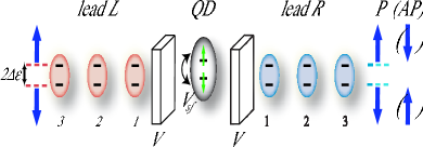
Figure 1: (Colour online) Schematic illustration of the model Hamiltonian. The lead $L$ with majority spin $\uparrow$ electrons and the lead $R$ with majority spin $\uparrow$ ($\downarrow$) electrons in the P (AP) configurations are separated from the QD by tunnel barriers which are accounted for with a renormalized hopping $V$. The energy-spin-splitting is $2\Delta\varepsilon$ in the leads and $2E_{z}$ in the QD. Spin-flip scatterings of strength $V_{sf}$ occur in the QD.

$$\varepsilon_{\alpha j\sigma} = (-1)^{\delta_{\sigma,\downarrow}}\Delta\varepsilon\quad\quad\quad\quad\quad\quad\mathrm{P\quad}$$

$$\varepsilon_{\alpha j\sigma} = (-1)^{\delta_{\alpha,L}}(-1)^{\delta_{\sigma,\downarrow}}\Delta\varepsilon\quad\quad\;\mathrm{AP\quad}$$ (2)

where $2\Delta\varepsilon$ is the band spin splitting. In the above model the P configuration corresponds to a majority-spin electron with spin $\uparrow$ in both leads, while in the AP configuration the majority-spin electron have spin $\uparrow$ in lead $L$ and spin $\downarrow$ in lead $R$. The case of normal leads corresponds to $\Delta\varepsilon=0$. The Hamiltonian of the quantum dot reads

$$H_{QD}=\sum_{\sigma}\varepsilon_{d\sigma}d^{\dagger}_{\sigma}d_{\sigma}+V_{sf}d^{\dagger}_{\uparrow}d_{\downarrow}+V_{sf}^{*}d^{\dagger}_{\downarrow}d_{\uparrow}\,,$$ (3)

where $d^{(\dagger)}_{\sigma}$ annihilates (creates) an electron on the QD with spin $\sigma$ and $V_{sf}$ is responsible for intra-dot spin-flip scatterings. The on-site energy $\varepsilon_{d\sigma}=\varepsilon_{d}+\sigma E_{z}/2$, $\sigma=\pm 1$, where $E_{z}$ is an intra-dot energy splitting. The quantum dot is connected to the leads via the tunneling Hamiltonian

$$H_{T}=\sum_{\alpha=L,R}\sum_{\sigma\sigma^{\prime}}\left(V_{d\sigma,\alpha\sigma^{\prime}}d^{\dagger}_{\sigma}c_{\alpha 1\sigma^{\prime}}+V_{d\sigma,\alpha\sigma^{\prime}}^{*}c^{\dagger}_{\alpha 1\sigma^{\prime}}d_{\sigma}\right)\,.$$ (4)

with $V_{d\sigma,\alpha\sigma^{\prime}}$ the amplitude for an electron in the QD with spin $\sigma$ to hop to the first site of lead $\alpha$ with spin $\sigma^{\prime}$. Alternatively, one can express $H_{T}$ in terms of the one-body eigenstates of $H_{\alpha}$ labelled by $(\alpha,k,\sigma)$,

$$H_{T}=\sum_{\alpha=L,R}\sum_{k=1}^{N}\sum_{\sigma\sigma^{\prime}}\left(V_{d\sigma,\alpha k\sigma^{\prime}}d^{\dagger}_{\sigma}c_{\alpha k\sigma^{\prime}}+V_{d\sigma,\alpha k\sigma^{\prime}}^{*}c^{\dagger}_{\alpha k\sigma^{\prime}}d_{\sigma}\right)\,,$$ (5)

with $V_{d\sigma,k\alpha\sigma^{\prime}}=\sqrt{2/(N+1)}\,V_{d\sigma,\alpha\sigma^{\prime}}\,\sin k$.

Putting all terms together the Hamiltonian of the whole system in equilibrium reads

$$H_{0}=H_{L}+H_{R}+H_{QD}+H_{T}\,.$$ (6)

In the next two Sections we study out-of-equilibrium properties of the system described in Eq.(6), after a sudden switch-on of a bias voltage $U_{\alpha}(t)$ in lead $\alpha=L,R$. We calculate the time-dependent spin-polarized current $I_{\alpha\sigma}(t)$ flowing between the QD and lead $\alpha$. $I_{\alpha\sigma}(t)$ is defined as the variation of the total number of particles $N_{\alpha\sigma}$ of spin $\sigma$ in lead $\alpha$,

$$I_{\alpha\sigma}(t)\equiv\frac{d}{dt}N_{\alpha\sigma}=2\Re\sum_{k,\sigma^{\prime}}V_{\alpha k\sigma,d\sigma^{\prime}}\,G^{<}_{d\sigma^{\prime},\alpha k\sigma}(t,t)\,,$$ (7)

where $G^{<}_{d\sigma^{\prime},\alpha k\sigma}$ is the dot-lead lesser Green’s function of the contacted non-equilibrium system, and $\Re$ stands for the real part. Unless otherwise stated, the current is computed at the $L$ interface and the short-hand notation $I_{\sigma}=I_{L\sigma}$ is used for the spin-polarized current while $I_{tot}=I_{\uparrow}+I_{\downarrow}$ and $I_{spin}=I_{\uparrow}-I_{\downarrow}$ denote the total current and spin current respectively. We further specialize to constant biases $U_{\alpha}(t)=U_{\alpha}$, except in Section IV.2 where the bias is a periodic pulse. Therefore we define $U\equiv U_{L}$, while the value of $U_{R}$ is either 0 or $-U$. The numerical simulations have been performed using dot-leads hoppings independent of $\alpha$ (symmetric contacts). We show that, despite the symmetry between $L$ and $R$ leads, the sign of the steady-state TMR can be inverted, a property which has been so far ascribed to strongly asymmetric tunneling barriers.tsymbal ; rlxh.2007 Moreover we specialize Eq.(4) to the case $V_{d\uparrow,\alpha\uparrow}=V_{d\downarrow,\alpha\downarrow}\equiv V$, and $V_{d\uparrow,\alpha\downarrow}=V_{d\downarrow,\alpha\uparrow}=0$. However we note that spin-flip scatterings are accounted for by considering a finite intra-dot $V_{sf}$ which is taken to be real in this work. If not otherwise specified, the initial Fermi energy $E_{F}$ of both leads is set to 0 (half-filled electrodes). In the numerical calculations below all energies are measured in units of $V_{0}$ ($4V_{0}$ is the bandwidth of the leads), times are measured in units of $\hbar/V_{0}$ and currents in units of $eV_{0}/\hbar$ with $e$ the electron charge.

III Results in the wide band limit approximation

Here we study the model introduced in the previous Section within the WBLA. This approximation has been mostly used to study spinless electrons and a closed formula for the exact time-dependent current has been derived.jahuo ; stefanucci Below we generalize these results to systems where the spin symmetry is broken. The retarded Green’s function projected onto the QD can be expressed in terms of the embedding self-energy

$$\Big{(}\Sigma(\omega)\Big{)}_{\sigma\sigma^{\prime}}=\sum_{\nu=\uparrow,\downarrow}\,\sum_{\alpha=L,R}\Big{(}\Sigma_{\alpha\nu}(\omega)\Big{)}_{\sigma\sigma^{\prime}}$$ (8)

which is a $2\times 2$ matrix in spin space. In Eq.(8) $(\Sigma_{\alpha\nu})_{\sigma\sigma^{\prime}}$ accounts for virtual processes where an electron on the QD hops to lead $\alpha$ by changing its spin from $\sigma$ to $\nu$, and hops back to the QD with final spin $\sigma^{\prime}$. Exploiting the Dyson equation the expression of $(\Sigma_{\alpha\nu})_{\sigma\sigma^{\prime}}$ is

$$\Big{(}\Sigma_{\alpha\nu}(\omega)\Big{)}_{\sigma\sigma^{\prime}}=\sum_{k}\,V_{d\sigma,\alpha k\nu}\,g_{\alpha k\nu}(\omega)\,V_{\alpha k\nu,d\sigma^{\prime}}\,,$$ (9)

where $g_{\alpha k\nu}=(\omega-\varepsilon_{\alpha k\nu}-U_{\alpha}+i\eta)^{-1}$ is the retarded Green’s function of the uncontacted $\alpha$ lead expressed in term of the one-particle eigenenergies $\varepsilon_{\alpha k\nu}$. In the WBLA Eq.(9) becomes

$$\Big{(}\Sigma_{\alpha\nu}(\omega)\Big{)}_{\sigma\sigma^{\prime}}\approx-\frac{i}{2}\Big{(}\Gamma_{\alpha\nu}\Big{)}_{\sigma\sigma^{\prime}}\,,$$ (10)

i.e., the self-energy is independent of frequency. The $2\times 2$ matrices $\Gamma$’s have the physical meaning of spin-dependent tunneling rates and account for spin-flip processes between the leads and the QD. We wish to point out that each $\Gamma$ matrix must be positive semi-definite for a proper modeling of the WBLA. Indeed, given an arbitrary two dimensional vector $(v_{\uparrow},v_{\downarrow})$ one finds

$$\sum_{\sigma,\sigma^{\prime}}v^{*}_{\sigma}\Big{(}\Gamma_{\alpha\nu}\Big{)}_{\sigma\sigma^{\prime}}v_{\sigma^{\prime}}=2\pi\sum_{k}\delta(\omega-\varepsilon_{\alpha k\nu}-U_{\alpha})\Big{|}\sum_{\sigma}V_{d\sigma,\alpha k\nu}v_{\sigma}\Big{|}^{2}\,.$$ (11)

The above condition ensures the damping of all transient effects in the calculation of local physical observables.

Proceeding along similar lines as in Ref.stefanucci, one can derive an explicit expression for spin-polarized current $I_{\alpha\sigma}(t)$ defined in Eq.(7),

$$I_{\alpha\sigma}(t)=I_{\alpha\sigma}^{s}+\int\frac{d\omega}{2\pi}\,f(\omega)\,\mathrm{Tr}\Big{[}T_{\alpha}(\omega,t)\Gamma_{\alpha\sigma}\Big{]}\,,$$ (12)

$f(\omega)$ being the Fermi distribution function. In the above equation $I_{\alpha\sigma}^{s}$ is the steady-state polarized current which for $\alpha=L$ reads

$$I_{L\sigma}^{s} = \int\frac{d\omega}{2\pi}\,\Big{(}f(\omega-U_{L})-f(\omega-U_{R})\Big{)}$$

$$\times \mathrm{Tr}\Big{[}\frac{1}{\omega-H_{QD}+\frac{i}{2}\Gamma}\Gamma_{R}\frac{1}{\omega-H_{QD}-\frac{i}{2}\Gamma}\Gamma_{L\sigma}\Big{]}$$

with $\Gamma_{\alpha}=\sum_{\sigma}\Gamma_{\alpha\sigma}$ and $\Gamma=\sum_{\alpha}\Gamma_{\alpha}$. The steady current at the right interface $I_{R\sigma}^{s}$ is obtained by exchanging $L\leftrightarrow R$ in the r.h.s. of Eq.(LABEL:ssl). We observe that $I_{R\sigma}^{s}\neq-I_{L\sigma}^{s}$ since the spin current is not conserved in the presence of spin-flip interactions. The second term on the r.h.s. of Eq.(12) describes the transient behavior and is expressed in terms of the quantity

$$T_{\alpha}(\omega,t) = \sum_{\beta}U_{\beta}\frac{e^{i(\omega+U_{\beta}-H_{QD}+\frac{i}{2}\Gamma)t}}{(\omega-H_{QD}+\frac{i}{2}\Gamma)(\omega+U_{\beta}-H_{QD}+\frac{i}{2}\Gamma)}\Big{[}i\delta_{\alpha,\beta}-\Gamma_{\beta}\,\frac{1}{\omega+U_{\beta}-H_{QD}+\frac{i}{2}\Gamma}\Big{]}+{\rm h.c.}$$ (14)

$$- \sum_{\beta}U_{\beta}^{2}\frac{e^{-i(H_{QD}-\frac{i}{2}\Gamma)t}}{(\omega-H_{QD}+\frac{i}{2}\Gamma)(\omega+U_{\beta}-H_{QD}+\frac{i}{2}\Gamma)}\,\Gamma_{\beta}\,\frac{e^{i(H_{QD}+\frac{i}{2}\Gamma)t}}{(\omega-H_{QD}-\frac{i}{2}\Gamma)(\omega+U_{\beta}-H_{QD}-\frac{i}{2}\Gamma)}\,.$$

Few remarks about Eq.(14) are in order. In linear response theory only the contribution of the first line remains. Such contribution is responsible for transient oscillations which are exponentially damped over a timescale $|\tau_{j}|$ and have frequencies $\omega_{\alpha j}\sim|E_{F}+U_{\alpha}-h_{j}|$, where $h_{j}+i\tau_{j}^{-1}$, $j=1,2$, are the two eigenvalues of $H_{QD}+i\Gamma/2$. These oscillations originate from virtual transitions between the resonant levels of the QD and the Fermi level of the biased continua (resonant-continuum). No information about the intra-dot transitions (resonant-resonant) is here contained. Resonant-resonant transitions are instead described by the contribution of the second line of Eq.(14) which yields oscillations of frequency $\omega_{1,2}=|h_{1}-h_{2}|$ damped as $\exp(-t/\tau_{1,2})$ with $\tau_{1,2}^{-1}=|\tau_{1}|^{-1}+|\tau_{2}|^{-1}$. Finally, it is straightforward to verify that for $\Gamma_{\alpha}$ and $H_{QD}$ both diagonal in spin space, Eq.(12) decouples into two identical formulae (but with different parameters), which exactly reproduce the well-known spinless result.jahuo ; stefanucci

Below we consider diagonal matrices $\Gamma_{\alpha\nu}$, in agreement with the discussion at the end of Section II. Thus, all spin-flip scatterings occur in the quantum dot. The ferromagnetic nature of the leads is accounted for by modeling the $\Gamma$ matrices asrud

$$\mathrm{P} \quad\left\{\begin{array}[]{ccc}\Big{(}\Gamma_{\alpha\uparrow}\Big{)}_{\uparrow\uparrow}&=&\Gamma_{0\alpha}(1+p)\quad\quad\alpha=L,R\\ \Big{(}\Gamma_{\alpha\downarrow}\Big{)}_{\downarrow\downarrow}&=&\Gamma_{0\alpha}(1-p)\quad\quad\alpha=L,R\\ \end{array}\right.$$ (17)

$$\mathrm{AP} \quad\left\{\begin{array}[]{ccc}\Big{(}\Gamma_{L\uparrow}\Big{)}_{\uparrow\uparrow}&=&\Gamma_{0L}(1+p)\\ \Big{(}\Gamma_{L\downarrow}\Big{)}_{\downarrow\downarrow}&=&\Gamma_{0L}(1-p)\\ \Big{(}\Gamma_{R\uparrow}\Big{)}_{\uparrow\uparrow}&=&\Gamma_{0R}(1-p)\\ \Big{(}\Gamma_{R\downarrow}\Big{)}_{\downarrow\downarrow}&=&\Gamma_{0R}(1+p)\\ \end{array}\right.$$ (22)

where all the remaining matrix elements are vanishing and $0<p<1$ is proportional to the polarization of the leads. Moreover we assume that $\Gamma_{0\alpha}\equiv\Gamma_{0}$ does not depend on $\alpha$, yielding a Left/Right symmetry in absence of ferromagnetism.

III.1 Normal case: quantum beats

In this Section we consider a quantum dot with an intra-dot energy splitting $E_{z}$ between the $\uparrow$ and $\downarrow$ levels, and an intra-dot spin-flip energy $V_{sf}$. The QD is coupled to $L$ and $R$ normal electrodes, $p=0$. The spin splitting $E_{z}$ leads to two different transient frequencies and produces coherent quantum beats in both the total and spin currents.souza The effect of spin-flip scatterings on the coherent oscillations is studied.

To make contact with Ref.souza, , we consider the same parameters, i.e. $U_{L}=0$, $U_{R}=200$, $\varepsilon_{d\sigma}=\theta(t)U_{R}/2+\sigma E_{z}/2$ with $E_{z}=10$, $\Gamma_{0}=1$ and inverse temperature $\beta=100$. However the intra-dot spin-flip coupling $V_{sf}$ is, in our case, non zero. In Fig.2 we show the time-dependent current $I_{tot}(t)$ and the discrete Fourier transform,stefanucci2 $I_{tot}(\omega)$, of $I_{tot}(t)-I_{tot}(\infty)$ for different values of $V_{sf}=0,\,10,\,20$. The spin current $I_{spin}(t)$ is displayed in Fig.3. The small tunneling rate $\Gamma$ leads to a very long transient regime, a property which allows us to observe well defined structures in the Fourier spectrum of the current. At $V_{sf}=0$ the frequencies of both $I_{\uparrow}(t)$ and $I_{\downarrow}(t)$ are $\omega_{\alpha 1}=\omega_{\alpha 2}=|U_{R}/2\pm E_{z}/2|=95,105$, in agreement with the results of Ref.souza, . This is confirmed by the Fourier analysis of $I_{tot}$ which is displayed in panel b) of Fig.2. As $V_{sf}$ is increased the frequencies of the transient oscillations change according to $|U_{R}/2\pm\sqrt{E_{z}^{2}/4+V_{sf}^{2}}|$, see panels d) and f) of Fig.2, and the amplitude of the quantum beats in $I_{tot}$ and $I_{spin}$ is suppressed. Such suppression is due to the fact that the Hamiltonian of the whole system is spin-diagonal if we choose the quantization axis along

$$\hat{\xi}=\hat{z}\cos\theta+\hat{x}\sin\theta\,,$$ (23)

with $\cos\theta=E_{z}/\sqrt{E_{z}^{2}+4V_{sf}^{2}}$. This follows from the invariance of the normal electrode Hamiltonians ($p=0$) and of the tunneling Hamiltonian ($\Gamma_{\alpha\sigma}=\Gamma_{0}\mbox{\boldmath$1$}_{2\times 2}$) under rotations in spin-space. Therefore, the time-dependent spin current measured along $\hat{z}$ is smaller the larger $V_{sf}$ is. Of course the spin current measured along the quantization axis $\hat{\xi}$ is not suppressed by changing $V_{sf}$.

Despite the quantum beats phenomenon and its suppression with increasing $V_{sf}$ are well captured within the WBLA, only a sub-set of transient frequencies can be predicted in this approximation. To describe transitions between the top/bottom of the electrode bands and the resonant levels requires a more realistic treatment of the leads Hamiltonian, see Section IV.

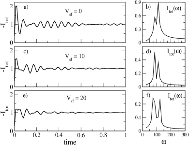
Figure 2: $I_{tot}(t)$ and $I_{tot}(\omega)$ for $V_{sf}=0$ [panels a)-b)], $V_{sf}=10$ [panels c)-d)], $V_{sf}=20$ [panels e)-f)]. The discrete Fourier transform is calculated using 50 equidistant points of $I_{tot}(t)-I_{tot}(\infty)$ with $t$ in the range (0.5,1). The rest of the parameters are $U_{L}=0$, $U_{R}=200$, $\varepsilon_{d\sigma}=\theta(t)U_{R}/2+\sigma E_{z}/2$ with $E_{z}=10$, $\Gamma_{0}=1$ and inverse temperature $\beta=100$.

Figure 3: (Colour online) $I_{spin}(t)$ for $V_{sf}=0,\,10,\,20$ and the same parameters as in Fig.2.

III.2 Ferromagnetic case: TMR

The finite spin-polarization $p$ of the electrodes breaks the invariance of $H_{L}$ and $H_{R}$ under rotations in spin-space. Thus the one-particle states become true spinors for nonvanishing $V_{sf}$. Using Eq.(LABEL:ssl) we calculate the steady-state total currents both in the P and AP configurations, which we denote as $I_{P}$ and $I_{AP}$, and study the TMR,

$$\mathrm{TMR}=\frac{I_{P}-I_{AP}}{I_{AP}}\,.$$ (24)

For $V_{sf}=0$ the TMR is always positive and its sign can be inverted only during the transient regime at sufficiently low temperatures.souza The positiveness of the steady state TMR is due to the fact that $\Gamma_{0L}=\Gamma_{0R}$. It is possible to show that for $\Gamma_{0L}\gg\Gamma_{0R}$ (or $\Gamma_{0L}\ll\Gamma_{0R}$) and $\varepsilon_{d\sigma}=0$, the $\mathrm{TMR}\approx-p^{2}$ in linear response theory yielding the so-called resonant inversion of the TMR.tsymbal

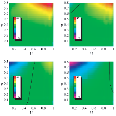
Figure 4: (Colour online) Contour plot of the TMR at the steady-state in units of $10^{-2}$ as a function of $U$ and $p$ for different values of $V_{sf}=0.3$ (top-left), 0.33 (top-right), 0.4 (bottom-left), 0.47 (bottom right). The boundary TMR $=0$ is displayed with a black line. The remaining parameters are $\Gamma_{0}=0.5$, $\varepsilon_{d\sigma}=0$, $\beta=100$.

In Fig.4 we display the contour plot of the TMR in the parameter space spanned by the bias voltage $U=U_{L}=-U_{R}$ and the polarization $p$ for different values of the spin-flip energy $V_{sf}$ and for $E_{z}=0$, $\Gamma_{0}=0.5$ and $\beta=100$. We observe that by increasing $V_{sf}$, a region of negative TMR appears and becomes wider the larger $V_{sf}$ is. The region in which the TMR is appreciably different from zero ($|\mathrm{TMR}|\gtrsim 0.05$ ) is confined to the high magnetization regime, i.e. $p\gtrsim 0.4$. The minimum of the TMR is reached for the largest value of $V_{sf}$ at small $U$ and large $p$, see panel d) of Fig.4. For small biases the sign inversion of the TMR can be understood by calculating the currents $I_{P}$ and $I_{AP}$ in linear response. By expanding Eq.(LABEL:ssl) to first order in $U$ and using the $\Gamma$ matrices of Eq.(22) one can show that to leading order in the bias

$$\mathrm{TMR}=p^{2}\frac{(1-p^{2})\Gamma_{0}^{4}-(1-p^{2})\Gamma_{0}^{2}V_{sf}^{2}-2V_{sf}^{4}}{[V_{sf}^{2}+(1-p^{2})\Gamma_{0}^{2}][(1+p^{2})V_{sf}^{2}+(1-p^{2})\Gamma_{0}^{2}]}\,.$$ (25)

For any given $V_{sf}$ and $\Gamma_{0}$ the denominator in the above expression is positive while the numerator can change sign. The regions of posite/negative TMR are displayed in the left side of Fig.5. For $\Gamma_{0}^{2}<2V_{sf}^{2}$ the TMR is negative independent of the polarization $p$. This follows from the fact that the tunneling time is larger than the time for an electron to flip its spin, thus favoring the AP alignment. Along the boundary $\Gamma_{0}^{2}=2V_{sf}^{2}$ the TMR is zero only for $p=0$ and negative otherwise. In the region $\Gamma_{0}^{2}>2V_{sf}^{2}$ there exists a critical value of the polarization,

$$p_{c}=\sqrt{1-\frac{2V_{sf}^{4}}{\Gamma_{0}^{4}-\Gamma_{0}^{2}V_{sf}^{2}}}\,,$$ (26)

such that the TMR is positive for $p>p_{c}$ and negative for $p<p_{c}$. It is worth to emphasize that at the boundary $V_{sf}=0$ the TMR is positive for any finite value of $p$ and zero for $p=0$. This analysis clearly shows that the sign of the TMR can be reversed without resorting to asymmetric couplings $\Gamma_{L}\neq\Gamma_{R}$, provided spin-flip processes are included. The right side of Fig.5 displays the TMR as a function of the polarization for different values of the ratio $V_{sf}^{2}/\Gamma_{0}^{2}<1/2$ (region of TMR inversion).

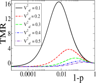
Figure 5: (Colour online) Left panel: in the region $\Gamma_{0}^{2}<2V_{sf}^{2}$ the TMR is always negative while in the region $\Gamma_{0}^{2}>2V_{sf}^{2}$ the TMR changes sign depending on the value of the polarization $p$. Right panel: TMR as a function of $p$ for $\Gamma_{0}=1$ and different values of $V_{sf}$.

We also have investigated the temperature dependence of the TMR. This is relevant in the light of practical applications, where a large TMR is desirable at room temperature. The increase of temperature tends to suppress the negative values of the TMR while the positive values remain almost unaffected. When $\beta\approx 1$ the region of the TMR inversion disappears. The positiveness of the TMR at high temperatures has been already observed in Ref.rud, .

In the next Section we provide an exact treatment of the 1D leads and illustrate differences and similarities with the results obtained so far.

IV Results for one-dimensional leads

The numerical results contained in this Section are obtained by computing the exact time-evolution of the system in Eq.(6) with a finite number $N$ of sites in both $L$ and $R$ leads. finiteleads1 ; finiteleads2 ; finiteleads3 Let us define the biased Hamiltonian at positive times as

$$H_{bias}(t)=H_{0}+H(t)$$ (27)

with

$$H(t)=\theta(t)\sum_{\sigma=\uparrow,\downarrow}\sum_{j=1}^{N}U_{\alpha}(t)c^{\dagger}_{\alpha j\sigma}c_{\alpha j\sigma}\,.$$ (28)

Both $H_{0}$ and $H_{bias}$ have dimension $2(2N+1)$, where the factor of 2 accounts for the spin.

We use the partition-free approachcini and specialize to a sudden switching of a constant bias. Accordingly, we first calculate the equilibrium configuration by numerically diagonalizing $H_{0}$, and then we evolve the lesser Green’s function as

$$G^{<}(t,t^{\prime})=ie^{-iH_{bias}t}f(H_{0})e^{iH_{bias}t^{\prime}}\,,$$ (29)

with $f$ the Fermi distribution function. The spin-polarized current flowing across the bond $m-n$ is then calculated from

$$I_{m,n,\sigma}(t)=2\sum_{\sigma^{\prime}}[H_{0}]_{m\sigma;n\sigma^{\prime}}\,\Im\{-i[G^{<}(t,t)]_{n\sigma^{\prime};m\sigma}\}\,,$$ (30)

where $[\dots]_{m\sigma;n\sigma^{\prime}}$ denotes the matrix element associated to site $m$ with spin $\sigma$ and site $n$ with spin $\sigma^{\prime}$, while $\Im$ stands for the imaginary part. The above approach allows us to reproduce the time evolution of the infinite-leads system provided one evolves up to a time $T_{max}\approx 2N/v$, where $v$ is the maximum velocity for an electron with energy within the bias window. Indeed for $t\gtrsim T_{max}$ high-velocity electrons have time to propagate till the far boundary of the leads and back yielding undesired finite-size effects in the calculated current, see Fig.6. For this reason we set $N$ much larger than the time at which the steady state (or stationary oscillatory state in the case of AC bias) is reached. We tested this method by comparing our numerical results against the ones obtained in Refs.stefanucci3, ; stefanucci2, where the leads are virtually infinite, and an excellent agreement was found for $t\lesssim T_{max}$. Moreover, the value of the current at the steady-state agrees with the Landauer formula with high numerical accuracy.

Below we study the spin-polarized current at the left interface $I_{\sigma}=I_{1L,d,\sigma}$ flowing between the first site of the lead $L$ ($m=1L$) and the QD ($n=d$) with spin $\sigma$. We stress that our approach is not limited to the calculation of the current through a specific bond, as we have access to the full lesser Green’s function. Sensible electron densities and currents in the vicinity of the QD can be extracted and their calculation requires the same computational effort.

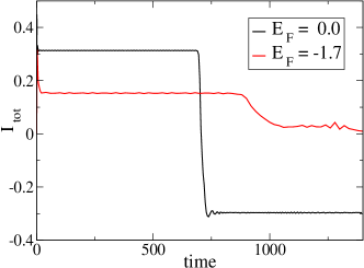
Figure 6: (Colour online) $I_{\uparrow}(t)$ at zero temperature for $N=700$, $U_{L}=0.5$, $U_{R}=0$, $E_{F}=0$ ($T_{max}\approx 700$), and $E_{F}=-1.7$ ($T_{max}\approx 870$). The rest of the parameters are $\varepsilon_{d\sigma}=0$, $V=-1$, $V_{sf}=0$. The current reaches a well-defined steady state before the occurrence of finite-size effect ($t\gtrsim T_{max}$).

IV.1 Normal case: quantum beats

We study the quantum beats phenomenon for normal 1D leads ($\Delta\varepsilon=0$) and intra-dot spin-splitting $E_{z}$ for different values of the spin relaxation energy $V_{sf}$. The comparison between the results obtained within the WBLA and with 1D tight-binding leads will turn out to be very useful to elucidate advantages and limitations of the former approach.

In Fig.7 we show the time-dependent currents $I_{tot}(t)$ and its discrete Fourier transform $I_{tot}(\omega)$ at zero temperature using the parameters $U_{L}=0.7$, $U_{R}=0$, $V=0.03$, $\varepsilon_{d\sigma}=\theta(t)U_{L}/2+\sigma E_{z}/2$, with $E_{z}=0.04$, for different values of $V_{sf}=0,\,0.05,\,0.1$. The spin-current for the same parameters is displayed in Fig.8. The value of the dot-lead hopping $V$ corresponds to an effective (energy-dependent) tunneling rate $\Gamma$ of the order of $10^{-3}$. Thus both the bias and the energy spin-splitting are of the same order of magnitude as the ones used in Section IV if measured in units of $\Gamma$. As expected the current reaches a steady-state in the long time limit, since the bias is constant and $H_{bias}$ does not have bound states.finiteleads2 ; stefbound However, the weak links between the QD and the leads allows us to study a pseudo-stationary regime, in which the current displays well-defined quantum beats.

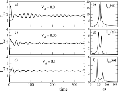
Figure 7: (Colour online) $I_{tot}(t)$ and $I_{tot}(\omega)$ for $V_{sf}=0$ [panels a)-b)], 0.05 [panels c)-d)], 0.1 [panels e)-f)] obtained with a bias $U_{L}=0.7$, $U_{R}=0$ applied to leads of length $N=450$. The discrete Fourier transform is calculated using 280 equidistant points of $I_{tot}(t)-I_{tot}(\infty)$ with $t$ in the range (70,350). The rest of the parameters are $V=0.03$, $\varepsilon_{d\sigma}=\theta(t)U_{L}/2+\sigma E_{z}/2$, $E_{z}=0.04$ and zero temperature.

Figure 8: (Colour online) $I_{spin}(t)$ for the same system parameters of Fig.7.

At $V_{sf}=0$, the dominant frequency of the spin-polarized current $I_{\uparrow}$ is $\omega^{0}_{\uparrow}=|U_{L}/2+E_{z}/2|\approx 0.37$ while $I_{\downarrow}$ oscillates with a dominant frequency $\omega^{0}_{\downarrow}=|U_{L}/2-E_{z}/2|\approx 0.33$, see panel b) of Fig.7. As in the WBLA, the difference between $\omega_{\uparrow}$ and $\omega_{\downarrow}$ leads to quantum beats in both $I_{tot}$ and $I_{spin}$ [see panel a) of Fig.7 and Fig.8]. For nonvanishing $V_{sf}$ the two fundamental frequencies $\omega^{0}_{\sigma}$ renormalizes as $\omega^{0}_{\sigma}\rightarrow\omega_{\sigma}=|U_{L}/2+\sigma\sqrt{E_{z}^{2}/4+V_{sf}^{2}}|$. The system Hamiltonian is no longer diagonal along the quantization axis $\hat{z}$ and $I_{\sigma}$ acquires the second frequency $\omega_{-\sigma}$ besides the original (but renormalized) one $\omega_{\sigma}$. We also observe that as $V_{sf}$ increases, the amplitude of the quantum beats in $I_{tot}$ and $I_{spin}$ is suppressed, similarly to what happen by treating the leads in the WBLA.

We would like to end this Section by pointing out that, for leads with a finite bandwidth the current might display extra oscillation frequencies corresponding to transitions either from or to the top/bottom of the bands, an effect which cannot be captured within the WBLA. We have investigated this scenario by changing the input parameters in such a way that the transitions from the resonant level of the QD to the bottom of the band are energetically favored. We set $U_{R}=0.4$, $U_{L}=0$, $E_{z}=0$, $E_{F}=-1.8$, $\varepsilon_{d}=-0.5$, $V=0.02$ and $V_{sf}=0$. The corresponding (spin-independent) current and its Fourier spectrum are shown in Fig.9. One can clearly see two well defined peaks at energies $\omega_{1}\approx 1.3$ and $\omega_{2}\approx 1.5$. As expected, one of these frequencies corresponds to a transition from the resonant level to the Fermi energy of the $L$ lead, i.e. $|E_{F}-\varepsilon_{d}|=1.3$. Transitions between the resonant level and the Fermi energy of the $R$ lead, i.e. $|E_{F}+U_{R}-\varepsilon_{d}|=0.9$, are strongly suppressed since the current is measured at the $L$ interface. Thus the second peak has to be ascribed to a transition which involves the bottom of the band $E_{B}=-2$, specifically the transition of energy $|E_{B}-\varepsilon_{d}|=1.5$. This kind of features in the Fourier spectra of the transients points out the limitations of the WBLA and might be experimentally observed in QD’s connected to narrow-band electrodes.

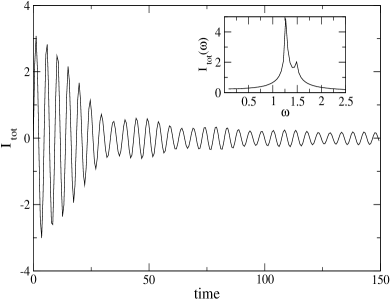
Figure 9: $I_{tot}(t)$ in units of $10^{-6}$ for $U_{R}=0.4$, $U_{L}=0$ applied to leads of length $N=250$. The inset shows $I_{tot}(\omega)$ in units of $10^{-5}$ calculated using 138 equidistant points of $I_{tot}(t)-I_{tot}(\infty)$ with $t$ in the range (12,150). The rest of the parameters are $E_{z}=0$, $E_{F}=-1.8$, $\varepsilon_{d}=-0.5$, $V=0.02$, $V_{sf}=0$ and zero temperature.

IV.2 Normal case: engineering the spin-polarization

In this Section we exploit the full knowledge of the time-dependent response of the system in order to engineer the spin-polarization of the total current. In particular we are interested in maintaining the polarization ratio

$$r(t)=2\frac{I_{tot}(t)I_{spin}(t)}{I_{tot}^{2}(t)+I_{spin}^{2}(t)}$$ (31)

above some given value in a sequence of time windows of desired duration. The quantity $r$ is $\pm 1$ for fully polarized currents and zero for pure charge or spin currents.

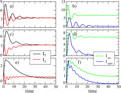
Figure 10: (Colour online) Currents in units of $10^{-2}$ for $U_{L}=-U_{R}=1$ applied to leads of length $N=120$ for different values of $E_{z}=0.1$ [panels a)-b)], 0.6 [panels c)-d)], 2 [panels e)-f)]. The rest of the parameters are $V=0.2$, $V_{sf}=0$ and zero temperature.

In Fig.10 we show the time-dependent currents $I_{\uparrow}(t)$ and $I_{\downarrow}(t)$ as well as $I_{tot}(t)$ and $I_{spin}(t)$ at zero temperature for different values of $E_{z}=0.1,\,0.6,\,2$ and $U_{L}=-U_{R}=1$, $V=0.2$, and $V_{sf}=0$. In the long-time limit the values of $r$ increases steadily as $E_{z}$ is increased, and remains below $10^{-1}$ for $E_{z}\lesssim 2$. The polarization ratio can, however, be much larger in the transient regime and its maximum has a nontrivial dependence on $E_{z}$. At finite values of $E_{z}$ there is an initial unbalance of the spin up and down densities. This implies that for small times $I_{\downarrow}$ is suppressed and delayed with respect to $I_{\uparrow}$, since spin $\uparrow$ electrons can freely flow while there cannot be any spin $\downarrow$ flow before the initial spin $\downarrow$ electrons have left the QD.souza This is the so called Pauli blockade phenomenon and is responsible for a recoil of $I_{\downarrow}$ during the rise of $I_{\uparrow}$. In panel a)-b) of Fig.10 we consider the case $E_{z}=0.1$. Both $I_{\uparrow}$ and $I_{\downarrow}$ overshoot their steady-state value and oscillate with rather sharp maxima and minima during the initial transient, see panel a) of Fig.10. However, the oscillation frequencies are very similar (small $E_{z}$) and the time at which $I_{\uparrow}$ has a maximum in correspondence to a minimum of $I_{\downarrow}$ occurs when the amplitude of their oscillations is already considerably damped. On the other hand, for $E_{z}=0.6$, see panel c)-d) of Fig.10, there is a synergy between the Pauli blockade phenomenon and the frequency mismatch. At small $t$ such synergy generates large values of the ratio $r\approx 1$ despite $r(t\rightarrow\infty)$ is vanishingly small. By increasing further the value of $E_{z}$ we observe a long overshoot of $I_{\uparrow}$ while $I_{\downarrow}$ oscillates with high frequency, see panel e)-f) of Fig.10 where $E_{z}=2$. The ratio $r(t)$ is a smooth decreasing function of time for $t\gtrsim 3$ and approaches the value of about $10^{-2}$ for $t\rightarrow\infty$. This behavior differs substantially from the one obtained for $E_{z}=0.6$ where $r(t)$ has a sharp peak for $0\lesssim t\lesssim 3$ and is very small otherwise. Below we show how one can exploit this kind of transient regimes to maintain persistently a large value of $r$.

We consider the optimal case $E_{z}=0.6$ and apply a pulsed bias with period $T$ and amplitude $U_{L}=-U_{R}=1$ in lead $L$ and $R$ respectively. The period $T$ of $H_{bias}$ is tailored to maintain the polarization ratio $r(t)$ above $\sim 0.5$ in a finite range of the period. For time-dependent biases Eq.(29) has to be generalized, as the evolution operator is no longer the exponential of a matrix. We discretize the time and calculate the lesser Green’s function according to

$$G^{<}(t_{n},t_{n})\approx e^{-iH_{bias}(t_{n})\Delta t}\,G^{<}(t_{n-1},t_{n-1})\,e^{iH_{bias}(t_{n})\Delta t}\,,$$ (32)

where $t_{n}=n\Delta t$, $\Delta t$ is the time step, $n$ is a positive integer and $G^{<}(0,0)=if(H_{0})$.

In Fig.11 we plot two time-dependent responses for $T=6$ and $T=8$. The pulsed bias produces an alternate $I_{tot}$ and $I_{spin}$ whose amplitude depends on $T$. We note that the amplitude of $I_{tot}$ is of the same order of magnitude of the steady state value $I_{tot}(t\rightarrow\infty)$ attained in Fig.10 panel d) for constant bias. On the contrary the amplitude of $I_{spin}$ is two orders of magnitude larger than the corresponding steady-state value. The polarization $r$ cannot be maintained as large as $r\approx 1$ (maximum value of $r$ during the transient) due to an unavoidable damping. However, the value of $r$ is above 0.5 in a time window of 1.4 for $T=6$ (with a maximum value $r\sim 0.75$) and $2.6$ for $T=8$ (with a maximum value $r\sim 0.9$) in each period, see Fig.11.

Figure 11: (Colour online) $I_{tot}(t)$ and $I_{spin}(t)$ in units of $10^{-2}$ for a pulsed bias of period $T=6$ (top-left panel) and $T=8$ (bottom-left panel) of amplitude $U_{L}=-U_{R}=1$ applied to leads of length $N=120$. The polarization ratio $r(t)$ is displayed in the right panel. The rest of the parameters are the same as in Fig.10. The dotted lines in the left panel denote the pulsed bias in the left lead in units of $10^{-1}$. The numerical calculations have been performed with $\Delta t=0.1$.

IV.3 Ferromagnetic case: TMR

The spin-dependent band-structure of the leads introduces another frequency dependence in the currents. Both $I_{\uparrow}$ and $I_{\downarrow}$ display a coherent oscillation of frequency $\omega_{1,2}=|h_{1}-h_{2}|=2\sqrt{E_{z}^{2}/4+V_{sf}^{2}}$, where $h_{1,2}$ are the eigenvalues of the isolated QD. Such behavior cannot be observed in the normal case, as the model is diagonal along the quantization axis $\hat{\xi}$ of Eq.(23) and no transitions between states of opposite polarization along $\hat{\xi}$ can occur. In Fig.12 we display the spin-up current at zero temperature in the P configuration for $\Delta\varepsilon=1.5$, $U_{L}=1$, $U_{R}=0$, $\varepsilon_{d\sigma}=\theta(t)U_{L}/2+\sigma E_{z}/2$, $E_{z}=0.04$, $V=0.02$, and $V_{sf}=0.1$. Besides the frequencies $\omega_{L1}=|E_{F}+U_{L}-h_{1}|\approx 0.6$ and $\omega_{L2}=|E_{F}+U_{L}-h_{2}|\approx 0.4$ already discussed in Section III.1, one can see the appearance of the new frequency $\omega_{1,2}\approx 0.2$.

Figure 12: $I_{\uparrow}(t)$ in units of $10^{-4}$ for $U_{L}=1$, $U_{R}=0$ applied to leads of length $N=350$. The inset shows the discrete Fourier transform $I_{\uparrow}(\omega)$ calculated using 265 equidistant points of $I_{\uparrow}(t)-I_{\uparrow}(\infty)$ with $t$ in the range (35,300). The rest of the parameters are $\varepsilon_{d\sigma}=\theta(t)U_{L}/2+\sigma E_{z}/2$, $E_{z}=0.04$, $V=0.02$, $V_{sf}=0.1$ and zero temperature.

Next, we study the steady-state regime in both the P and AP configurations and calculate the TMR for different values of the bias voltage $U$, the band spin splitting $\Delta\varepsilon$ and the spin-flip energy $V_{sf}$. Analogies and differences with the case of wide-band leads will be discussed.

In Fig.13 we display the contour plot of the TMR in the parameter space spanned by the bias voltage $U=U_{L}=-U_{R}$ and the band-spin-splitting $\Delta\varepsilon$ at inverse temperature $\beta=100$, $V=0.5$, $\varepsilon_{d\sigma}=0$ and for $V_{sf}=0,\,0.25,\,0.5$. In the left panel we show the TMR for $V_{sf}=0$. We can see that despite the dot-leads link is symmetric, there is a finite region at small bias and intermediate $\Delta\varepsilon$ in which the TMR $<0$, although rather small ($\approx-0.05$). This is a new scenario for the TMR inversion and stems from the finite bandwidth of the leads (we recall that TMR $>0$ for $V_{sf}=0$ in the WBLA). The largest positive value of the TMR (TMR $\approx 0.7$) occurs for large magnetization and bias, as expected.

As $V_{sf}$ is increased (central and right panels of Fig.13) the region of positive TMR widens, which is an opposite behavior to the one in the WBLA. However, we note that the largest value of negative TMR occur at small $U$ and large $\Delta\varepsilon$ (TMR $\approx-0.2$, see right panel of Fig.13) and that the TMR changes sign abruptly as $U$ is increased, a feature which is in common with the WBLA. The positive values of the TMR reduce with respect to the case $V_{sf}=0$. This property is due to the presence of spin-flip scatterings which close conducting channels in the P configuration and open new ones in the AP configuration, thus suppressing the difference $I_{P}-I_{AP}$.

Finally we have investigated the dependence of the above scenario on temperature. It is observed that the qualitative picture described in Fig.13 survives down to $\beta\approx 10$. Increasing further the temperature the TMR behaves similarly to the WBLA.

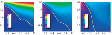
Figure 13: (Colour online) Contour plot of the TMR at the steady-state in units of $10^{-2}$ as a function of $U$ and $\Delta\varepsilon$ for different values of $V_{sf}=0$ (left), 0.25 (center), 0.5 (right). The boundary TMR $=0$ is displayed with a white line. The remaining parameters are $V=0.5$, $\varepsilon_{d\sigma}=0$, $\beta=100$ and the length of the leads is $N=100$.

V Summary and conclusions

The ultimate goal of future QD-based devices is the possibility to generate spin-polarized currents, control their spin-coherence time, and achieve high TMR after the application of high-frequency signals. This calls for a deep understanding of the time-dependent responses in these systems.

In this paper we have calculated spin-dependent out-of-equilibrium properties of lead-QD-lead junctions. Realistic transient responses are obtained within the partition-free approach. The time-dependent current is calculated for QDs connected to ferromagnetic leads and in the presence of an intra-dot spin flip interaction. This requires the propagation of a two-component spinor.

For 1D leads, we evolve exactly a system with a finite number $N$ of sites in each lead. If $N$ is sufficiently large, reliable time-evolutions are obtained during a time much larger than all the characteristic time-scales of the infinite system.finiteleads1 ; finiteleads2 ; finiteleads3 By comparing our results against the ones obtained with leads of infinite length,stefanucci3 ; stefanucci2 we have verified that our method is accurate and robust, beside being very easy to implement.

We have solved analytically the time-dependent problem in the WBLA and derived a closed formula for the spin-polarized current. Such formula generalizes the one obtained in the spin-diagonal case and has a transparent interpretation.souza ; souza2 We stress, however, that within the WBLA, transitions involving the top or the bottom of the leads band are not accounted for. The latter may be relevant to characterize, e.g, the coherent beat oscillations when the device is attached to narrow-band electrodes.

Furthermore we have shown how to engineer the transient response of the system to enhance the spin-polarization of the current through the QD. This is achieved by controlling parameters like, e.g., the external magnetic field, the transparency of the contacts, and imposing a pulsed bias of optimal period. It is shown that by exploiting the synergy between the Pauli-blockade phenomenon and the resonant-continuum frequency mismatch, one can achieve an AC spin-polarization two orders of magnitude larger than the DC one.

We also have employed the Stoner model to describe ferromagnetic leads and computed the steady-state TMR. We have found a novel regime of negative TMR, in which the geometry of the tunnel junction is not required to be asymmetric and a finite intra-dot spin-flip interaction turns out to be crucial. For any given $V_{sf}$ there is a critical value of the ferromagnetic polarization above which the TMR is negative. The magnitude of the TMR is very sensitive to temperature variations and the TMR inversion phenomenon disappears as $\beta$ approaches the damping-time of the system.

We would like to stress that our approach is not limited to 1D electrodes and can be readily generalized to investigate multi-terminal devices consisting of several multi-level QDs. Finally, owning to the fact that the propagation algorithm is based on a one-particle scheme, it prompts us to include electron-electron interactions at any mean-field level or within time-dependent density functional theory.rg.1984

VI Acknowledgements

E.P. is financially supported by Fondazione Cariplo n. Prot. 0018524. This work is also partially supported by the EU Network of Excellence NANOQUANTA (NMP4-CT-2004-500198).

References

- (1) D. D. Awschalom, D. Loss, and N. Samarth, Semiconductor Spintronics and Quantum Computation (Nanoscience and Technology Series), edited by K. von Klitzing, H. Sakaki, and R. Wiesendanger (Springer, Berlin, 2002).
- (2) D. Loss and D. P. DiVincenzo, Phys. Rev. A 57, 120 (1998).
- (3) J.M. Kikkawa, I.P. Smorchkova, N. Samarth, and D.D. Awschalom, Science 277, 1284 (1997).
- (4) J.M. Kikkawa and D.D. Awschalom, Phys. Rev. Lett. 80, 4313 (1998).
- (5) J. M. Elzerman et al., Nature (London) 430, 431 (2004).
- (6) M. Kroutvar et al., Nature (London) 432, 81 (2004).
- (7) T. Fujisawa, Y. Tokura and Y. Hirayama, Phys. Rev. B 63, R081304 (2001).
- (8) J. A. Gupta, D. D. Awschalom, X. Peng, and A. P. Alivisatos, Phys. Rev. B 59, R10421 (1999).
- (9) A. Greilich, R. Oulton, E. A. Zhukov, I. A. Yugova, D. R. Yakovlev, M. Bayer, A. Shabaev, Al. L. Efros, I. A. Merkulov, V. Stavarache, D. Reuter, and A. Wieck, Phys. Rev. Lett. 96, 227401(2006).
- (10) F. M. Souza, Phys. Rev. B 76 205315 (2007).
- (11) B, Naser, D.K. Ferry, J. Heeren, and J.L. Reno, J.P. Bird, Appl. Phys. Lett. 89, 083103 (2006).
- (12) M. Sharma, S.X. Wang, and J.H. Nickel, Phys. Rev. Lett. 82, 616 (1999).
- (13) J. M. De Teresa, A. Barthélémy, A. Fert, J. P. Contour, F. Montaigne, and P. Seneor, Science 286, 507 (1999).
- (14) A. N. Pasupathy, R. C. Bialczak, J. Martinek, J. E. Grose, L. A. K. Donev, P. L. McEuen, and D. C. Ralph, Science 306, 86 (2004).
- (15) E. Y. Tsymbal, A. Sokolov, I. F. Sabirianov, and B. Doudin, Phys. Rev. Lett. 90 186602 (2003).
- (16) T.-S. Kim, Phys. Rev. B 72, 024401 (2005).
- (17) Y. Ren, Z.-Z. Li, M.-W. Xiao, and A. Hu, Phys. Rev. B 75, 054420 (2007).
- (18) M. Cini, Phys. Rev. B 22, 5887 (1980).
- (19) G. Stefanucci and C. O. Almbladh, Phys. Rev. B 69, 195318 (2004).
- (20) F. M. Souza, A. P. Jauho, J. C. Egues, arXiv:cond-mat/08020982 (unpublished).
- (21) Y. Ren, Z.-Z. Li, M.-W. Xiao, and A. Hu, Phys. Rev. B 75, 054420 (2007).
- (22) A.-P. Jauho, N.S. Wingreen, and Y. Meir, Phys. Rev. B 50, 5528 (1994).
- (23) W. Rudzińsky, and J. Barnaś, Phys. Rev. B 64 085318 (2001).
- (24) G. Stefanucci, S. Kurth, A. Rubio, and E. K. U. Gross, Phys. Rev. B 77, 075339 (2008).
- (25) N. Bushong, N. Sai, and M. Di Ventra, Nano Lett. 5, 2569 (2005).
- (26) A. Dhar, and D. Sen, Phys. Rev. B 73, 085119 (2006).
- (27) A. Agarwal and D. Sen, J. Phys.: Condens. Matter 19, 046205 (2007).
- (28) S. Kurth, G. Stefanucci, C.-O. Almbladh, A. Rubio, and E. K. Gross, Phys. Rev. B 72, 035308 (2005).
- (29) G. Stefanucci, Phys. Rev. B 75, 195115 (2007).
- (30) F. M. Souza, S. A. Leão, R. M. Gester, and A. P. Jauho, Phys. Rev. B 76 125318 (2007).
- (31) E. Runge and E. K. U. Gross, Phys. Rev. Lett. 52, 997 (1984).