Production and decays of the light pseudoscalar boson
at the LHC
in the simplest little Higgs model
Abstract
In many extensions of the standard model, the Higgs sector often contains an additional pseudoscalar boson. A good example is the SU(3) simplest little Higgs model, which accommodates a light pseudoscalar boson with quite different characteristics from those in other multi-Higgs-doublet models. We study various phenomenological signatures of the at the LHC. In particular, we calculate in details both production and decays in the Drell-Yan type channel , and in the associated production with a pair, . We emphasize the decay mode of the boson when its mass is below the threshold. We show that production is in fact large enough to give a sizable number of events while suppressing the backgrounds. We also comment on the direct gluon fusion process and the indirect decay from the heavy quark ().
I Introduction
One of the primary goals of the CERN Large Hadron Collider (LHC) is to understand the electroweak symmetry breaking, which is vital in explaining the origin of the fermion and gauge boson masses. In the standard model (SM), one single Higgs doublet is introduced to trigger the electroweak symmetry breaking, of which the by-product is a scalar boson known as the Higgs boson. Although the SM does not predict the mass of the Higgs boson (), we have direct, indirect, and theoretical bounds on . The most up-to-date search has placed a lower bound of 114.4 GeV LEP on . The precision measurements from LEP and SLD collaborations have placed an upper bound on GeV (at one-sided 95% C.L.) prec , which is much lighter than the theoretical one (the so-called triviality bound) of about 1 TeV. The consensus is that the Higgs boson is rather light.
The SM by itself cannot provide any theoretical framework to guarantee the lightness of the Higgs boson. Very often small masses are protected by some symmetries, e.g., the chiral symmetry to protect fermion masses and the gauge symmetry to protect gauge boson masses. There are no such symmetries in the SM to protect the scalar boson masses. A recent class of models, dubbed the little Higgs models, has been developed based on the idea that the lightness of the Higgs boson is attributed to its being a pseudo Nambu-Goldstone boson (pNGB) LH . Armed by the collective symmetry breaking idea, little Higgs models can explain the little hierarchy problem. The Higgs boson mass is radiatively generated with quadratic divergence emerging at two loop level: The Higgs boson mass around 100 GeV and the 10 TeV cut-off are possible without fine-tuning. The one-loop level quadratic divergences from the SM gauge boson and top-quark loops are canceled by those from new heavy gauge boson and heavy -quark loops, respectively. According to the global symmetry breaking pattern little Higgs models can be classified into two categories: (i) the product group models where the diagonal breaking of two (or more) gauge groups leads to the SM gauge group, and (ii) the simple group models where a single larger gauge group is broken into the SM gauge group. The most studied product group model is the littlest Higgs model littlest while that for the simple group model is the simplest little Higgs model simplest . In this work, we focus on the simplest little Higgs (SLH) model, which generates the least fine tuning in explaining the low Higgs mass fine-tuning .
A special feature of the simplest little Higgs model is the presence of a light pseudoscalar boson, denoted by . The model is based on [SU(3) U(1) global symmetry with its diagonal subgroup SU(3) U(1)X gauged. The vacuum expectation values (VEV) of two SU(3)-triplet scalar fields, , spontaneously break both the global symmetry and the gauge symmetry. Uneaten pNGB’s consist of a SU(2)L doublet and a pseudoscalar . In Ref. cheung-song it was pointed out that the boson in the original model is massless, which is problematic for production in rare and decays, - mixing, and , as well as for the cosmological axion limit. One of the simplest remedies was suggested by introducing a term into the scalar potential by hand simplest ; Kaplan:Schmaltz ; Kilian:pseudo-scalar . This term then determines the mass. The mass of is not theoretically constrained, but there exists an experimental constraint from non-observation in the decay . It excludes pseudoscalar bosons with mass below 5–7 GeV heavyQ . It has been also shown that a sizable portion of parameter space kinematically allows the decay , which can relieve the constraint on the direct search bound on the Higgs boson mass cheung-song ; cheung-song-yan .
In this work, we focus on production and decays of a light boson at the LHC. The decay pattern of is quite similar to that of the SM Higgs boson. A few distinctive features are (i) the does not decay into and , (ii) has a rather large branching ratio into , and (iii) the dominant decay mode is if kinematically allowed. The largest production channel for is gluon fusion, but the decay of will be buried under QCD backgrounds while will not likely stand out of the Drell-Yan background. The fusion does not contribute to production. Associated production with pair and with the Higgs boson could be the most useful channels to search for the .
The organization is as follows. In the next section, we describe briefly the simplest little Higgs model with the term. We calculate the decays and production of the boson in Sec. III and IV, respectively. We study the detection of the boson in Sec. V and VI. We then conclude in Sec. VII.
II simplest group model with the term
The SU(3) simplest little Higgs model is based on global symmetry with its diagonal subgroup gauged. The symmetry breaking of is generated by aligned VEVs of two complex SU(3) triplet scalar fields, and . Out of the 10 degrees of freedom in and , five are eaten by the SU(3) symmetry breaking. Remained five degrees of freedom in are parameterized as a nonlinear sigma model with
| (1) |
where and
| (2) |
Radiatively generated VEV of the Higgs boson field triggers the SM electroweak symmetry breaking (EWSB): The Higgs boson is defined by . Without resort to any expansion, and have the following closed form cheung-song :
| (3) |
Note that in is only a phase factor. Explicit form of are also useful for later discussions:
| (7) | |||||
| (11) |
The covariant derivative term is
| (12) |
where and is the tangent of the electroweak mixing angle. Detailed expressions for is referred to Ref. smoking . As and develop their VEVs, the 5 degrees of freedom appear as the longitudinal component of the heavy gauge bosons, including a gauge boson and a complex SU(2) doublet , with masses
| (13) |
For convenience we separate the Lagrangian in Eq. (12) into three terms:
Using Eq. (3) it is easy to see that the first term is just the kinetic term of the Higgs boson and :
| (15) |
The last term leads to the masses for the gauge bosons as well as the coupling of the Higgs boson with two gauge boson. Since is only a phase factor in , the -dependence in disappears. From Eqs. (3) and (7), the second term leads to only the --, --, and -- couplings:
where .
The fermion sector in this model should be extended since the gauged SU(3) symmetry promotes the SM fermions into SU(3) triplets. The Yukawa interaction of the third generation quarks is determined by the little Higgs mechanism which cancels the largest contribution of the top quark to the radiative Higgs mass . However negligible contributions to of the first two generation quarks and all generation leptons leave some ambiguity in fermion embedding. In the literature, two kinds of fermion embedding have been discussed, the “universal” embedding smoking , and the “anomaly-free” embedding kong . In this paper we focus on the anomaly-free embedding case. The universal embedding case has almost the same Yukawa couplings of , except that the first two generation heavy quarks are up-type while those in the anomaly-free embedding are down-type.
The quark Yukawa interactions for the third generation and for the first two generations are given by smoking
| (17) | |||||
| (18) |
where ; are SU(3) indices; and ; runs over ; runs over .
The mass eigenstate (, ) are the mixture of (, ), where and ,
| (19) |
where the quark sector is the same as the quark sector. The mixing angles are
| (20) |
where and .
The heavy quark masses (, , ) and the SM quark masses are
| (21) |
Small masses of and are satisfied simply by the condition , which implies
| (22) |
Accepting this simplification, this model has the following five parameters:
| (23) |
In Ref. cheung-song , it is shown that proper EWSB prefers rather large around 10.
Focused on , we put its Yukawa couplings as
| (24) |
where the index includes all of the SM fermions and heavy fermions, is the fermion mass, is the Higgs VEV, and is the heavy top partner. We ignore -- and -- couplings due to their small mixing angles in Eq.(22). The parameter indicates the ratio of the Yukawa coupling to the SM Higgs Yukawa coupling, given by
| (27) |
where .
III Decay
For , the decays dominantly into a pair of SM fermions that is kinematically allowed. The decay rate of is
| (28) |
where , and is the color factor of the fermion . Since has a factor of , a pseudoscalar boson with mass just above twice of a fermion mass has larger decay rate. Since the decay rate is proportional to the fermion mass, boson with mainly decays into a pair. In the following calculation of decay widths, we use the running mass of the quarks evaluated at the scale to calculate the Yukawa coupling, but not in the phase space factor. This is why the partial width into is smaller than that into .
As in the Higgs boson case, the radiative decay rates of into and are also important. Since has no coupling with the charged gauge bosons, the partial decay widths into and are, respectively,
| (29) | |||||
| (30) |
where , and are, respectively, the color factor and the electric charge of the fermion running in the loop. The dimensionless loop factor is
| (31) |
with
| (32) |
(a) (b)
(c)
For above the threshold the dominant decay mode is into the pair. However, due to huge QCD background it is very difficult to identify the boson in this mode, unless it is produced associated with some leptonic final states. The same difficulty is expected for . On the other hand, the decay mode into could be useful, especially for . In this mass range, about 50% branching ratio is possible for . We shall concentrate on this mode in Sec. V.
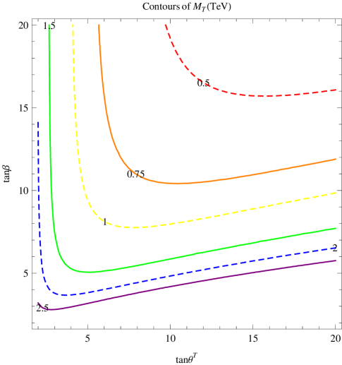
In Fig. 1, we show the dependence of on and . We have set TeV and TeV. Since proper EWSB can be achieved by large around 10, the heavy top mass is somewhat sensitive to : For , is relatively light below 1 TeV; for , becomes heavier above 1 TeV.
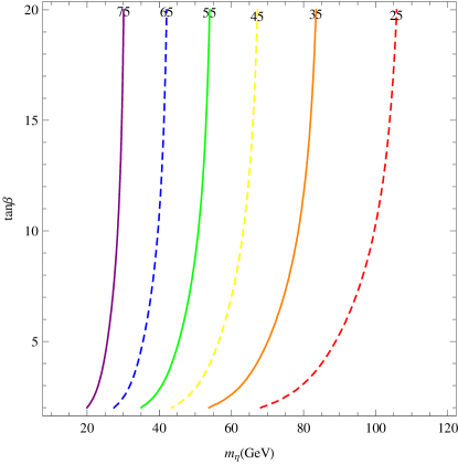
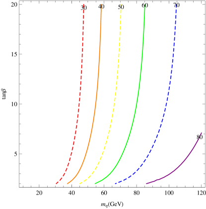
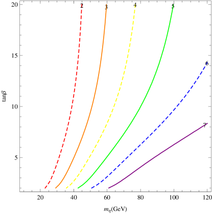
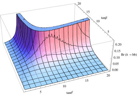
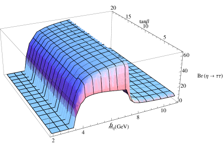
In Fig. 2 (a)–(c), we show the contours of Br, Br, and Br, respectively, in (, ) plane. The presented value for and is in unit of , while that for is in unit of . We vary GeV, and . The branching ratios are quite sensitive to , but relatively insensitive to . As in Fig. 1, we used GeV, TeV and TeV.
(a) (b)
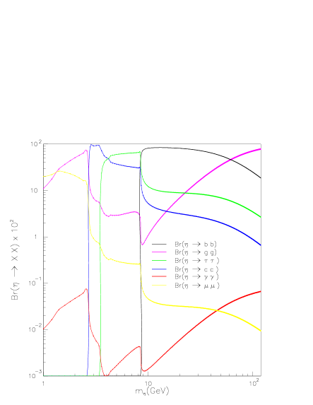
In Fig. 3, we show the branching ratios for the dominant decay modes of . For Br is the largest, whereas in the range Br is the largest. For , the largest is Br, followed by Br. When GeV, Br becomes dominant. As further increases, however, Br takes over. This is due to the enhancement from the contributions of heavy , and , which are non-decoupled in the triangle loops. Such an enhancement is helpful for production at the LHC via gluon fusion. On the other hand, Br is only at the level in most of the parameter space. This is due to the absence of the -coupling with charged gauge bosons.
IV production at the LHC
Main production channels for at the LHC are, in the order of the size of cross sections,
-
1.
gluon fusion: ;
-
2.
fusion: ;
-
3.
associated production with : ;
-
4.
associated production with : ; and
-
5.
decay from : and .
The resulting cross sections are to be compared in subsection F.
IV.1 Gluon fusion
For gluon fusion the cross section at hadron collider with the c.m. energy for the LHC) is
| (33) |
where , is the parton distribution function of a gluon inside a proton, and
| (34) |
IV.2 fusion
For the fusion the cross section is
where
| (36) |
IV.3 associated production
The process of is mediated by , , and gauge bosons. Since the gauge coupling of with the SM fermion is suppressed by and , we ignore it in the following. The interaction Lagrangian is parameterized by
| (37) |
where , , , and
| (38) | |||||
| (39) |
Here and .
For the process of
| (40) |
the parton level differential cross section is
| (41) |
where is the scattering angle of with respect to the incoming quark in the parton c.m. frame, , and . The effective couplings are
| (42) |
The cross section of collision is then
where is the parton density of inside the hadron .
IV.4 associated production
There are two contributing subprocesses:
The latter dominates at the LHC energy because of large gluon luminosity. We write down the helicity amplitudes in the appendix, and use FORM to evaluate the square of the amplitudes.
IV.5 In the decay
A pair of is produced by QCD interactions, similar to a top-quark pair. When the is heavy enough, single- production is kinematically advantageous SingleT . In little Higgs models, the heavy quark decays dominantly into , , and smoking . When neglecting final-state masses over , the partial decay rates are
| (44) |
where
| (45) |
Here . If these are the only decay modes of , the branching ratios of would show simple relation of . However the SLH model allows another important decay mode of . Its partial decay rate is
| (46) |
Since EWSB prefers large so that is suppressed if is not as large as , this decay mode can be important. For example, two benchmark points in Ref.cheung-song-yan have sizable decay rate of : in the SHL-A case and in the SHL-B case.

In Fig. 4, we show the production cross section of a single heavy top at the LHC, multiplied by its branching ratio for . We fix and vary and in the range between 6 and 12. We have included the single- production as well as the single- production. As stressed in Ref.SingleT , the non-negligible process of with its charge-conjugated production is also included. Only for very optimal case of around 500 GeV, the production from the decay can reach 1 pb.
IV.6 Comparisons
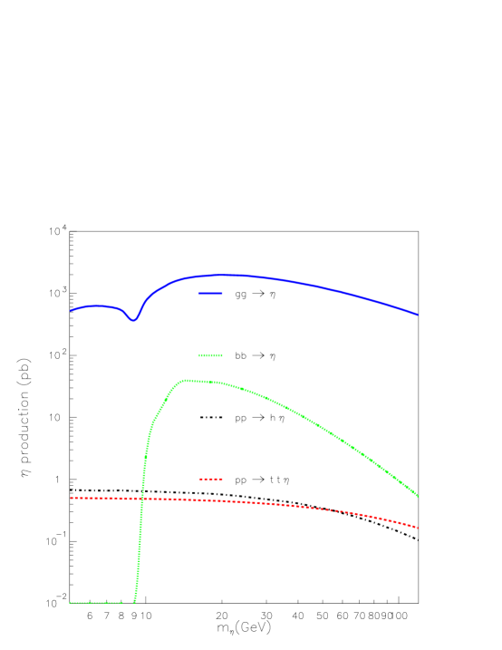
In Fig. 5, we show the production cross sections against the mass of the for various production channels at the LHC. The most dominant production channel is the gluon fusion, followed by the fusion. In both channels, there is only in the final state, which will decay into either a pair or pair depending on . Both modes suffer, respectively, from large QCD background and the Drell-Yan background. We do not consider these two production channels in the subsequent sections. In the associated production of , one has the addition decay to put the handle on. We will study this channel in detail in the next section. Another channel of interest is the . We will consider the signal-background in Sec. VI. Finally, one should not ignore the ’s from the decay of the heavy . As long as is not too heavy such that its production rate is sizable, we expect enough ’s from decays.
V The signal and background of the process
In this section, we study the signal and backgrounds of the production associated with the Higgs boson. To enhance the signal, we consider the following mass ranges of and where the subsequent decay of and are important:
| (47) |
Then production has the dominant decay mode of without missing transverse energy. The kinematic cuts imposed on ’s and ’s are
| (48) |
The reconstruction efficiencies of and are taken as and , respectively. The rejection rates of gluon and light quarks faking are taken as , while the rejection rate of quark faking is taken as tau . To simulate the detector effects, we smear the energies of the jets and ’s with the following Gaussian resolutions
| (49) | |||||
| (50) |
where are measured in GeV. We also introduce the following invariant mass cuts on and to suppress the backgrounds:
| (51) |
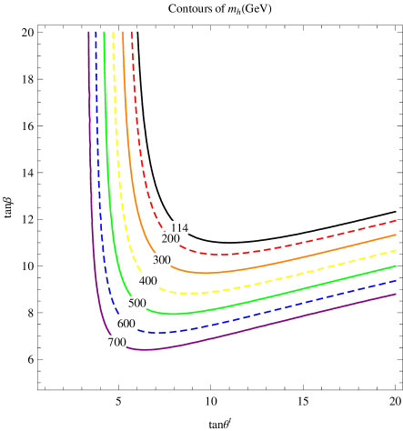
To further suppress the background from , we reject events with the missing transverse energy GeV, which is about the threshold of the missing transverse energy signature of CMS and ATLAS detectors. We observe that this cut can reduce the background by . For Fig. 6, we present the Higgs mass and its branching ratio into in the plane of and with fixed . The branching ratio Br is given in Fig. 7, which is almost insensitive to the value of .
(a) (b)
In order to simulate the signal, we select the following benchmark point:
| (52) |
The relevant physics quantities corresponding to this benchmark point are GeV, Br, GeV, GeV, Br and Br. The -- coupling in Eq. (II) is about at the benchmark point. The small branching ratio of is due to the small . At this benchmark point, the is quite heavy and does not appreciably contribute to .
We have several comments on the decay properties of and in the mass region .
-
1.
The main decay channels of are and . The branching ratio of is the largest due to the fact that QCD corrections to Br encoded in the running mass make it substantially smaller than that of Br, even though the pole mass of charm quark is close to tau pole mass and this channel has a color factor of 3. In this mass region, the branching ratio Br is not sensitive to the parameter .
-
2.
The mass of Higgs is not sensitive to the change of due to the smallness of .
-
3.
The decay mode of is small unlike the case in Refs. cheung-song ; cheung-song-yan , because here the mass of is small and the decay rate is proportional to .
(a) (b)
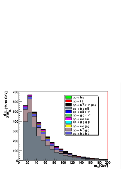
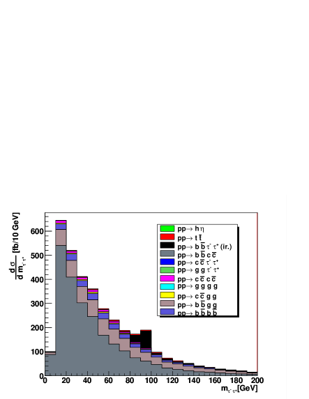
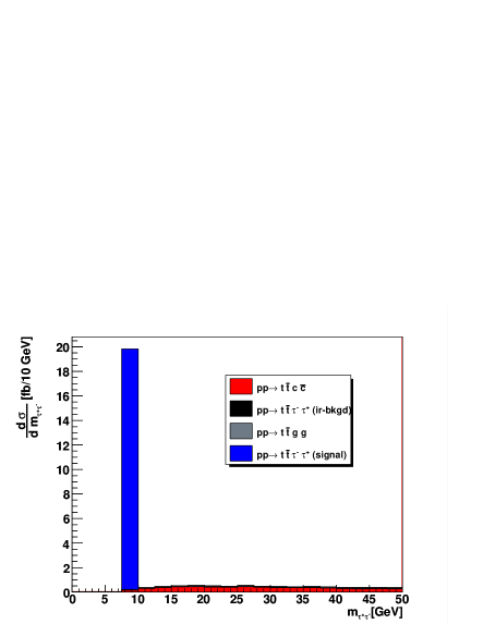
In Fig. 8, we show the signal and various backgrounds in both and invariant mass distributions. It is clear that the signal is buried under the background and can hardly be seen. From these two plots, we can identify that the is the most dominant background. In order to separate the signal of it is crucial to enhance the rejection factor for quark faking . The final signal and background rates are tabulated in Table 1.
| Background processes | Cross Section (fb) |
| Signal processes | Cross Section (fb) |
A few more comments on the signal are in order here.
-
1.
The raw cross section of is around pb. With the branching ratios of Br and Br, the signal is around fb. After imposing the cuts on , , and , the signal is reduced to fb. In addition, the cuts on ’s and ’s further reduce the signal to fb, because most of events are lost due to the cut on the not-so-energetic ’s and the cut in each signal event. Considering the reconstruction efficiencies and the invariant mass cuts given in Eq. (51), the final reconstructed cross section is fb.
-
2.
When we fix and increase , we find that the final reconstructed cross section decreases. For instance when we take GeV, the reconstructed cross section is only fb. This reduction is not only due to the decrease of the cross section but also due to the onset of the mode .
-
3.
Unlike MSSM and NMSSM, there is no dramatic enhancement due to large for the than the chosen benchmark point in Eq.(52). First the parameter has an upper bound by the validity of perturbation expansion cheung-song . Second, the coupling of -- is around half of , which is almost the maximum value in the allowed parameter space. Third, the branching ratio of Br cannot change drastically with the increase of . This is to be compared with the MSSM and NMSSM model cases where both the -- coupling and the branching ratio of Br might be enhanced by factors of and , respectively.
VI The signal and backgrounds of
In this section we study the signal and backgrounds of , focused on the benchmark point in Eq. (52). For simplicity we first assume that the reconstruction efficiency of the top quark is percent and can be fully reconstructed. We can focus on the analysis of the signal and the most direct backgrounds at the and level. The majority of backgrounds comes from with , among which is the most serious background. This is because of poor rejection factor of the charm quark, which behaves similarly to a -jet. Another source of background is , which is irreducible but essentially small because the ’s are produced mostly off a virtual photon or a boson.
We note that the invariant mass cut on is very crucial for signal event selection. It removes most of irreducible backgrounds, in which the two ’s are emitted from a virtual photon, , or a Higgs boson. It also suppresses the background effectively. In Fig. 9, we show the spectrum of for both the signal and the major backgrounds. It is obvious that the signal clearly stands out of the backgrounds.
| Background processes | Cross Section (fb) |
| Signal processes | Cross Section (fb) |
In Table 2, we show the cross sections of major backgrounds and signal after cuts. Here we comment on the signal in more detail. The total cross section of the process is about fb. After imposing the kinematic cuts on the ’s, the cross section is reduced to about fb. Including the reconstruction efficiency of ’s, it further reduces to about fb. Note that we have only analyzed down to the and level. If we take the top-quark decays into account, there should be more backgrounds such as jets and jets. However, these backgrounds are electroweak in nature and thus much smaller than the QCD production of .
The signal-to-background ratio seems quite promising. However, we still need to apply the top quark reconstruction and identification efficiencies. For a simple estimate of the top quark reconstruction, we should include the reconstruction efficiency of two jets and two ’s. With one of the ’s decaying leptonically ( and ) while the other one decaying hadronically, the reduction factor is therefore
| (53) |
where is the -tagging efficiency. Thus, the more realistic reconstructed cross section of is estimated to be fb. Even taking into account the selection cuts for the decay products of the top quark, we should still have enough signal events per LHC year.
VII Conclusions
We have performed a comprehensive study on the decays and production of the pseudoscalar boson of the simplest little Higgs model at the LHC. We focus on the mass range of such that the dominant decay mode is , followed by and . The decay branching ratio into is only of the order of .
The dominant production channel is gluon fusion (), followed by fusion (). However, the sole in the final state may be buried under the Drell-Yan background in this invariant mass region. We have therefore focused on the associated production channels of and . We have shown that production is in fact large enough to give a sizable number of events while suppressing the backgrounds, the majority of which comes from . On the other hand, suffers severely from the background. Unless experiments can achieve a very high rejection factor for charm quark, this channel remains pessimistic.
Appendix A Helicity amplitudes for and
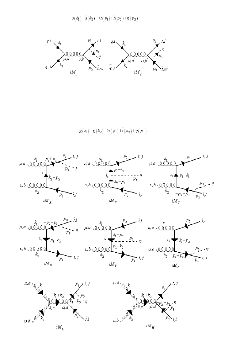
For the process of
there are two contributing Feynman diagrams, as shown in Fig. 10. Here the 4-momenta and the color indices () are given in parenthesis. The amplitudes are
where and the interaction Lagrangian is .
There are eight Feynman diagrams, as depicted in Fig. 10, contributing to the subprocess
where are color indices. The -channel-like helicity amplitudes are
| (54) |
The -channel-like ones are
| (55) |
The -channel-line ones are
where the constant factors are given by
Appendix B Decay of
The heavy gauge boson decays into the SM fermions () and into the Higgs and bosons (). We neglect the decay of since the vertex is suppressed by , without enhancement. In spite of non-suppressed -- and -- couplings, the mass relation of does not allow the decay of . Decay rates are
| (56) | |||||
where . We refer the expression of and ’s for to Eq. (38). Other couplings are
| (57) | |||||
Acknowledgements.
The work of JS is supported by the Korea Research Foundation Grant (KRF-2005-070-c00030). The work of KC, PT, and QSY is supported by the NSC under grant no. NSC 96-2628-M-007-002-MY3 and the NCTS.References
- (1) R. Barate et al. [LEP Working Group for Higgs boson searches], Phys. Lett. B 565, 61 (2003).
- (2) The LEP Electroweak Working Group, the latest result is in http://lepewwg.web.cern.ch/LEPEWWG/
- (3) N. Arkani-Hamed, A. G. Cohen and H. Georgi, Phys. Lett. B 513, 232 (2001); N. Arkani-Hamed, A. G. Cohen, E. Katz, A. E. Nelson, T. Gregoire and J. G. Wacker, JHEP 0208, 021 (2002); N. Arkani-Hamed, A. G. Cohen and H. Georgi, Phys. Lett. B 513, 232 (2001); M. Perelstein, arXiv:hep-ph/0512128.
- (4) N. Arkani-Hamed, A. G. Cohen, E. Katz and A. E. Nelson, JHEP 0207, 034 (2002);
- (5) M. Schmaltz, JHEP 0408, 056 (2004).
- (6) J. A. Casas, J. R. Espinosa and I. Hidalgo, JHEP 0503, 038 (2005).
- (7) K. Cheung and J. Song, Phys. Rev. D 76, 035007 (2007) [arXiv:hep-ph/0611294].
- (8) D. E. Kaplan and M. Schmaltz, JHEP 0310, 039 (2003).
- (9) W. Kilian, D. Rainwater and J. Reuter, Phys. Rev. D 71, 015008 (2005); Phys. Rev. D 74, 095003 (2006) [arXiv:hep-ph/0609119].
- (10) N. Brambilla et al. [Quarkonium Working Group], arXiv:hep-ph/0412158; W. M. Yao et al. [Particle Data Group], J. Phys. G 33 (2006) 1; R. Balest et al. [CLEO Collaboration], Phys. Rev. D 51, 2053 (1995).
- (11) K. Cheung, J. Song and Q. S. Yan, Phys. Rev. Lett. 99, 031801 (2007) [arXiv:hep-ph/0703149].
- (12) T. Han, H. E. Logan and L. T. Wang, JHEP 0601, 099 (2006).
- (13) O. C. W. Kong, arXiv:hep-ph/0307250; O. C. W. Kong, J. Korean Phys. Soc. 45, S404 (2004).
- (14) K. Cheung, C. S. Kim, K. Y. Lee and J. Song, arXiv:hep-ph/0608259.
- (15) G. Bagliesi et al., “Tau jet reconstruction and tagging at high level trigger and off-line,” CERN-CMS-NOTE-2006-028, Jan 2006.