sourav.sur@uleth.ca and saurya.das@uleth.ca
Multiple kinetic k-essence, phantom barrier crossing and stability
Abstract
We investigate models of dark energy with purely kinetic multiple k-essence sources that allow for the crossing of the phantom divide line, without violating the conditions of stability. It is known that with more than one kinetic k-field one can possibly construct dark energy models whose equation of state parameter crosses (the phantom barrier) at recent red-shifts, as indicated by the Supernova Ia and other observational probes. However, such models may suffer from cosmological instabilities, as the effective speed of propagation of the dark energy density perturbations may become imaginary while the barrier is crossed. Working out the expression for we show that multiple kinetic k-essence fields do indeed lead to a crossing dark energy model, satisfying the stability criterion as well as the condition (in natural units), which implies that the dark energy is not super-luminal. As a specific example, we construct a phantom barrier crossing model involving three k-fields for which is a constant, lying between and . The model fits well with the latest Supernova Ia Union data, and the best fit shows that crosses at red-shift , whereas the dark energy density nearly tracks the matter density at higher red-shifts.
pacs:
98.80.-k, 95.36.+x, 98.80.JK1 Introduction
The late-time accelerated expansion of the universe is now well established through the observations of the luminosity distance – red-shift relation for type Ia Supernovae (SNIa) [1, 2, 3, 4, 5, 6, 7, 8]. Measurements of the cosmic microwave background (CMB) temperature fluctuations by the Wilkinson Microwave Anisotropy Probe (WMAP) [9, 10] as well as the large scale red-shift data from the Sloan Digital Sky Survey (SDSS) [11] further indicate that the universe is very nearly spatially flat and consists of about of dark energy (DE) which drives the cosmic acceleration. The value of the DE equation of state (EoS) parameter, i.e., the ratio of pressure to energy density of DE, , should be less than to maintain this acceleration. Although the simplest candidate for DE is a cosmological constant (), for which , there are serious theoretical problems associated with it [12]. needs to be extremely fine tuned so that the DE at present is small compared to the Planck scale. A fine tuning is also required to keep the (-) dark energy density comparable with the present critical density , while the acceleration begins only in the recent past — the coincidence problem. From the observational point of view, although there are indications that is very close to at present, combined studies of SNIa, CMB and baryon acoustic oscillation (BAO) peaks do actually point toward a dynamical DE with EoS parameter slowly varying with red-shift . More specifically, the so-called CDM model, which consists of and cold dark matter as dominant components, although consistent with the low- observational data, does not produce sufficiently good fits with the data at relatively higher (). Accordingly, there have been a large number of model-independent and model-dependent DE parameterizations explored in the literature [13, 14, 15, 16, 17]. Extensive studies reveal that in parameterizing the DE to produce good fits with the observational data, it is always desirable to have no inherent restriction imposed on from the underlying theory. For instance, it is not desirable to have always , which is required for the theoretical consistency of many popular DE models, such as quintessence, tachyon, dilaton, etc. For the reviews on various dynamical aspects of DE, see [18].
Within the scope of minimally coupled canonical scalar field DE models, such as quintessence [19], the crossing from to can never happen and there is a need of more than one scalar field, at least one of which is of phantom nature, i.e., carries a wrong sign in front of the kinetic term [20]. For this reason the line is commonly known as the phantom divide line (PDL). Phantom fields violate the dominant energy condition, and therefore could give rise to classical instabilities [21]. Moreover, since the phantom energy density is unbounded from below, the quantum mechanical stability is in jeopardy. The vacuum is unstable against the decay into ghosts and positive energy particles, which couple to gravitons producing further decay into cosmic gamma rays [22]. In an expanding Friedmann universe, the extremely repulsive (anti-gravitating) nature of the phantom fields pose more problems as the phantom energy density generically tends to infinity in finite time in future leading to the so-called “Big Rip” singularity [23], as well as some other mild singularities. For a general categorization of these singularities see for instance [24].
Apart from the coupled quintessence and phantom models, commonly known as the quintom models [25], there are various other models in which the phantom barrier crossing is shown to be achieved in a consistent way. Notable among these are the scalar-tensor models [26], brane-world models [27], string-inspired dilatonic ghost condensate models [28], quantum-corrected Klein-Gordon models with quartic potential [29], coupled DE models [30], modified gravity models [31], H-essence (complex scalar) models [32], etc. In this work, we focus on the so-called k-essence models [33, 34], which incorporate a natural generalization of quintessence via a Lagrangian with non-linear dependence on the kinetic term(s) for the scalar field(s). For such models is not constrained to be and may in principle cross the PDL. However, it has been argued by Vikman [35] that in the case of a single field k-essence model, with a Lagrangian of the form , where is the kinetic term of the scalar field , the PDL crossing either leads to instabilities against cosmological perturbations or is realized by a discrete set of phase space trajectories111There are however some counter-arguments and counter-examples set in [36, 37] and it is shown that for a generalized single field k-essence Lagrangian of the form stable PDL crossing is indeed possible for some specific functional form of and .. For a multiple k-essence model, involving more than one k-fields , with kinetic terms , the PDL crossing is shown to be possible even when the Lagrangian is purely a function of the kinetic terms, [38]. However, the stability of such a model against cosmological perturbations have not been explored in the literature.
A major difficulty in dealing with the equations of scalar-type cosmological perturbations for multiple scalar fields is that these equations are extremely coupled in the curvature and isocurvature modes, even when the scalar fields are only minimally coupled to gravity [39, 40, 41, 42]. For multiple k-essence, the perturbation equations are complicated further, however there are some specific cases in which the expression for the speed of propagation of the curvature perturbations could be obtained and the stability analysis could be performed [43, 44]. For example, when the k-essence Lagrangian is , where and [43], the propagation speed is simply given by the well-known result of Garriga and Mukhanov [45], i.e., . On the other hand, in the multi-field Dirac-Born-Infeld (DBI) inflationary scenario, the propagation speed for the Lagrangian , is given in a homogeneous background by [44]. However, none of these expressions for will hold for the most general Lagrangian , corresponding to the non-interacting fields . A comprehensive study of the curvature perturbation equations reveals that one can, in principle, obtain the expression of for the multi k-field Lagrangian [46], leaving aside the isocurvature modes which couple weakly with the curvature mode in the large-scale limit [40, 41].
In this paper we first investigate whether the multiple kinetic k-essence DE models that allow the PDL crossing is cosmologically stable, i.e., the speed of propagation of the DE density perturbations satisfies the condition . It is also relevant to check whether (in natural units), so that the DE perturbations do not travel faster than light [47]. However, the requirement is not potentially stringent, because it has been argued that causal paradoxes do not necessarily arise even when [48]. We find that in most circumstances (including the model described in [38]) where dynamically varies with time, the PDL crossing is associated with a flip of sign of , thus giving rise to violent instability. An appropriate choice for in a stable DE model is therefore a constant whose value lies between and . Imposing this condition on we work out the constraint on the field configuration. As a specific example we try to construct a stable PDL crossing DE model using this constraint and with the least number of model parameters possible, so as to determine these parameters with less uncertainties by fitting with the observational data. While within the scope of two k-fields the stability constraint leads to complicated field solutions, we construct a reasonably simpler model involving three k-fields for which stable PDL crossing is possible.
We constrain the parameters of the model using the most recent data-set released by the Supernova Cosmology Project (SCP) team [7], viz., the “Union” compilation, which consists of SNIa reduced to usable data points after various selection cuts. Marginalizing over the Hubble constant , we find that the best fit value of the present matter density parameter , whereas the best fit DE EoS parameter crosses the PDL at red-shift , fairly in agreement with found in many model-independent DE parameterizations [49]. The minimized value of the statistic is found to be about , which shows an improvement of over the minimized for the CDM model found with the Union data-set [8]. The minimized per degree of freedom for the model discussed in this paper is , which is also marginally better than that found in [6] for the CDM model using the older SNIa data-set complied by Riess et al [4]. Additionally, we see that the best fit value of the DE density almost tracks the matter density over sufficiently longer red-shift range in the past until becoming dominant after . Thus the model provides a possible resolution of the coincidence problem. Extrapolation of the best fit to future epochs shows a tendency of to turn back towards after reaching a minimum value. Thus the phantom regime appears to be transient and future singularities, such as the Big Rip, may be avoided.
The present model also differs from the usual quintom model [25] implemented using two (or possibly more) scalar fields, (at least) one of which has a negative definite kinetic energy density (i.e., phantom), and as such the EoS parameter is less than , whereas the other field(s) has(have) positive definite kinetic energy (quintessence-type) and EoS parameter(s) greater than . The negative energy field comes to dominate at late times and is responsible for the PDL crossing. In the three-field k-essence model which we study, two of the k-fields have positive definite energy density, whereas the energy density of the third k-field is negative for a sufficiently longer time in the past and present, but may become positive in distant future, as found by extrapolating the best fit model parameters to future (negative) red-shifts. In that sense the third k-field may not be regarded as equivalent to an eternal phantom, and quantum mechanical instabilities may be avoided. None of the fields have EoS parameter less than , unlike quintom models. Moreover, the negative energy k-field is not responsible for the super-acceleration (), it is a positive energy k-field that causes the PDL crossing, again in contrast with what happens in quintom models.
This paper is organized as follows: in sec. 2 we describe the general framework of multiple k-essence DE models assuming that there are no mutual interactions between the individual k-fields. In sec. 3 we consider the simplistic case of purely kinetic multiple k-essence and show that only for more than one dynamical k-fields the PDL crossing is possible, although the field configuration is severely constrained by the stability criterion. We work out this constraint and choose the value of the speed of propagation of the DE density perturbations to be a constant, in order to have a stable PDL crossing multiple kinetic k-essence DE model. In sec. 4 we construct a specific multiple k-field model for which is constant, and crosses the PDL in recent past. In sec. 5 we fit this model with the Union SNIa data [7], to reconstruct phenomenologically the multiple k-essence Lagrangian. We conclude with a summary and open questions in sec. 6. In the Appendix, we work out the equations of scalar-type cosmological perturbations for a multiple k-essence field configuration so as to find the expression for the propagation speed .
2 General Formalism
Let us consider the following action in dimensions:
| (1) |
where is the gravitational coupling constant, is the Lagrangian density for perfect fluid matter, are a set of mutually non-interacting scalar fields, and where stands for the kinetic term of the scalar field :
| (2) |
is the k-essence Lagrangian density for the field .
We assume the space-time structure to be described by a spatially flat Robertson-Walker (RW) line-element
| (3) |
where is the scale factor which is normalized to unity at the present epoch . In such a space-time, the kinetic term reduces to , where the over-dot stands for . The field equations are the Friedmann equations given by
| (4) |
where is the Hubble expansion rate, and are the perfect fluid energy density and pressure respectively, and are the k-essence energy density and pressure respectively, given by
| (5) |
Considering the perfect fluid matter in the form of pressure-less dust (), the field equations integrate to give the matter energy density as , where is the present value of . From Eq.(4) one obtains the expression for the normalized Hubble rate:
| (6) |
where is the present value of the Hubble parameter and , are the present values of the critical density and matter density parameter respectively.
The equations of motion of the scalar fields are given as
| (7) |
and the mutually non-interacting individual field components satisfy the continuity equation:
| (8) |
where are the EoS parameters for the individual fields . The EoS parameter for the k-essence DE is thus given by
| (9) |
Using Eqs. (4) and (6) one can express the total EOS parameter in terms of :
| (10) |
The deceleration parameter is given by
| (11) |
For an accelerated expansion of the universe () the total EOS parameter should be less than , and as can be observed from Eq. (10), is further less than . Although the observations favour the value of to be very close to that for a cosmological constant (i.e., ) at present and in recent past, extensive studies show that better fits with observational data require a dynamical DE with substantially greater than at relatively higher red-shifts (). Moreover, for consistent statistical data fits it is not desirable to always have a theoretical restriction such as . In other words, the dynamical DE models that allow the PDL crossing are most suited for analyzing the observational data so as to determine the cosmic evolution history over the entire red-shift range that is probed. While such a crossing in minimally coupled scalar field DE models is associated with violent cosmological instabilities, one has to ensure that the instabilities never occur in the multiple k-essence DE models. For such models the expression of the square of the speed of propagation of curvature perturbations is found to be (see the Appendix for detailed derivation)
| (12) |
In the case of a single k-field (, say) the above Eq. (12) reduces to the well-known result [45]. The value of must be non-negative, for the stability of a model, and always be less than unity (in natural units) so that the DE perturbations do not travel faster than light.
In the next section we examine the plausibility of a stable PDL crossing in the multiple k-essence scenario, considering for simplicity the k-field Lagrangian to be purely kinetic in nature.
3 Purely kinetic multiple k-essence
When the k-essence Lagrangian is purely a function of the kinetic terms , i.e., , the equations of motion (7) for the scalar fields can be integrated at once to give
| (13) |
However, remembering that in Robertson-Walker space-time, one may observe that the expressions (5), (9) and (12), for , and respectively, remain invariant under a field redefinition . Hence the constants can effectively be set to unity, for all , and the above equation can be rewritten as
| (14) |
Now, using the definitions (5) of and , we can express the DE EoS parameter , Eq. (9), and the square of the propagation speed of perturbations , Eq. (12), as
| (15) |
For a transition from to , the quantity needs to vanish at the PDL cross-over scale factor .
In the case of a single scalar field , say, and , the PDL crossing implies that , i.e., either or or both must vanish. This is clearly not possible for any finite value of since from Eq.(14) we have .
For more than one k-fields the PDL crossing is in principle possible whenever the quantity at , i.e., , by Eq. (14). However, from Eq. (15) we find that the change of sign of as the line is crossed, implies a change of sign of sign of as well, unless the numerator and denominator of exactly cancel each other to give a value which never flips sign. For example, if is a function of some numerical power of , i.e., (for all ), as has been considered in ref. [38], there is always a flip of sign of associated with the PDL crossing. Therefore unless one chooses to be such a function of which does not change sign for any value of , instabilities are bound to be there even in multiple k-essence DE models. Moreover, we must have in order that the DE perturbations do not travel faster than light. The simplest possible choice of , appropriate for a stable and non-super-luminal DE model is
| (16) |
Of course, the limiting case implies a non-propagating DE (for example, due to a cosmological constant). For dynamic DE models we have .
Let us now denote
| (17) |
Eq. (14) reduces to
| (18) |
and the DE energy density takes the form
| (19) |
From these equations we find
| (20) |
where prime denotes . Eqs. (15) for and reduce to
| (21) |
We rewrite the expression for in the form
| (22) |
where the arbitrary functions satisfy the relation . With the choice (constant), we therefore have
| (23) |
While from Eq. (21) we see that the PDL crossing requires at , a stable k-field configuration is the one that solves the above equation (23). In the next section we construct a cosmologically stable PDL crossing DE model by suitably choosing a specific field configuration and a reasonably simplified ansatz to solve for , and . We fit the solutions to the latest SNIa Union data [7] in the subsequent section, show the plausible tracking of the dark energy density to the matter density in the past, avoidance of future singularities, and finally reconstruct the multiple kinetic k-essence Lagrangian.
4 Cosmologically stable PDL crossing multiple kinetic k-essence model
4.1 Two k-field configuration
Let us first consider a field configuration involving only two scalar fields:
| (24) |
From Eq. (23) we have
| (25) |
Let us assume a power-law solution for as
| (26) |
Plugging this in Eq. (20) and integrating, and using Eq. (19), we get the expressions for the energy density and the pressure corresponding to the field as
| (27) |
where is a constant.
Substituting Eq. (26) in Eq. (25) and eliminating we obtain
| (28) |
Integrating this we get the algebraic equation
| (29) |
where is an integration constant.
We look for the simplest possible solutions of the above equation (29), so that the cosmological quantities and (and hence the normalized Hubble expansion rate ) have reasonably simple forms which we can fit with the observational data.
Let us first take into account the cases or for either of which Eq. (29) is linear in . However, for , Eq. (29) gives , i.e., , which can never change sign for any finite value of . Therefore we rule out as a possible choice for a PDL crossing DE model. For , on the other hand, we obtain from Eqs. (26) and (29) that constant, i.e., the corresponding fields and are non-dynamical, and PDL crossing never happens either. Hence we rule out the choice as well.
We next consider the case for which Eq. (29) is quadratic in . Corresponding to , we have . The solution of Eq. (29) is given by
| (30) |
where we denote . From Eqs. (26) and (30) we see once again that the expression for cannot change sign, i.e., the PDL crossing is not possible.
We are therefore left with the choices of the parameter which render Eq. (29) to be cubic, quartic or even higher order algebraic equation in 222There are also the choices and for which Eq. (29) is quadratic in and respectively. However, the solution for corresponding to these choices is not qualitatively different from that corresponding to shown above. The PDL crossing can never take place either.. The solutions for are however very complicated and leads to messy expressions for the corresponding energy density. An inspection of Eq. (29) also reveals that the choices of for which Eq. (29) is even order (quadratic, quartic, etc.) in , can be ruled out anyway, because can in no way change sign when the power is an even integer. In a separate work which is in progress [50] we examine the cases for which Eq. (29) is cubic or higher order in . In the present paper, however, we choose to work with a simpler alternative by introducing one more k-field, in a way that Eq. (29) remains quadratic in , and the above solution (30) could be used.
4.2 Three k-field configuration
Let us now consider the following configuration that involves three scalar fields:
| (31) |
From Eq. (23) we have
| (32) |
The solution for is
| (33) |
whence from Eqs. (19) and (20) we find the energy density and the pressure corresponding to the field as
| (34) |
where is a constant.
Once again, we assume the power-law solution (26) for , so that the energy density and the pressure corresponding to the field are given by (27), and is related to through the relation (29). Similar to the case of two k-fields, it is easy to show that the PDL crossing never happens for three k-fields as well, if the parameter or so that Eq. (29) is linear in . We therefore resort to the choice for which Eq. (29) is quadratic in and the solution for is given by Eq. (30). Using Eqs. (26), (33) and (30) we obtain
| (35) |
For a PDL crossing at , , which implies that the parameters and should satisfy the relation
| (36) |
Thus a smooth crossing from a regime to a regime is indeed possible for the choice , provided one of the parameters and must be negative with respect to the other, i.e., . However, a negative value of implies an eternally negative definite kinetic energy density for the field . A negative value , on the other hand, does not necessarily imply a negative energy density for the field , which is derived below. We therefore choose to work with .
Let us now set , so that the DE perturbations are slowly propagating with speed , and for which Eq. (20) could be integrated easily. Using Eqs. (19) and (20) one then obtains the expressions for the energy density and pressure components due to the field as
| (37) |
where is a constant and we denote . Using Eqs. (27), (34) and (4.2) we write the expressions for the total dark energy density () and total pressure (), for the choice , as
| (38) |
where .
Now, from Eq. (6) we express the normalized Hubble rate () as
| (39) |
where and . Eliminating using the condition that at the present epoch , and , we obtain
| (40) | |||||
One may observe that the parameter should not be greater than in order that is real, and the model to be valid. Moreover, for positive fractional values of , for which the PDL crossing could take place, the range of validity of the model is up to a finite time in the future at which the scale factor is . Therefore, the lesser the positive fractional value of , the more the model could be extended to future epochs.
In what follows, we fit this model with the observational data so as to determine the parameters and , and finally reconstruct the Lagrangian components and using the best fit values of the parameters.
5 Fitting the model with observational data
We use the most recent SNIa data released by the SN Cosmology Project (SCP) team, viz., the Union data-set [7]. It consists of a total of SN samples analyzed from various sources, reduced to most reliable data points after different outlier rejection cuts and selection tests. These Union data includes large samples of SNIa from the older data-sets by Perlmutter et al, Tonry et al, Riess et al, and others [1, 2, 3, 4], SN Legacy Survey (SNLS) [5], as well as the distant SN observed by the Hubble Space Telescope (HST). The range of data extends up to red-shift , and the full data can be obtained at http://supernova.lbl.gov/Union.
These data provide the extinction-corrected distance modulus, given by
| (41) |
where is the apparent magnitude of the source SN and is the absolute magnitude. Theoretically, the apparent magnitude is expressed as
| (42) |
where is the Hubble free luminosity distance, which for a spatially flat universe is defined in terms of the present matter density parameter and the set of theoretical model parameters as
| (43) |
is the magnitude zero point offset given by
| (44) |
where is the Hubble constant in units of Km s-1 Mpc-1.
The theoretical distance modulus is defined by
| (45) |
where
| (46) |
is a nuisance parameter, independent of the data points, and has to be uniformly marginalized over (i.e., integrated out).
The likelihood of and the theoretical model parameters are determined by minimizing the quantity
| (47) |
where , are the total uncertainties on the data points. For the Union data-set [7] .
Now, the marginalization with respect to can be done by the following two-step procedure [51]:
2. Substituting this value of in Eq. (48) we obtain
| (50) |
Now instead of minimizing in Eq. (47), one can minimize in Eq. (50) with respect to and , since both the minimized values would be the same.
In the case of the three k-field () model discussed above, corresponding to the choice , we find good fits to the SNIa data for positive fractional values of , and with the negative sign of square roots appearing in the expression for in Eq. (40). We fit the observational data for two parametric choices of and , for which the model remains valid up to sufficiently large future red-shifts and respectively.
: With this choice we get the minimized value of for the Union data-set [7], and the best fit values . The minimized is better by from that found with the Union data for the two-parameter flat CDM model [7, 8]. The minimized per degree of freedom (dof) is also improved by from that found in ref. [6] by fitting the flat CDM model with the older SNIa gold data-set [4].
: With this choice we get the minimized , which is improved further by than that obtained for the previous choice (). The best fit values of the present matter density parameter and the model parameters are obtained as: .
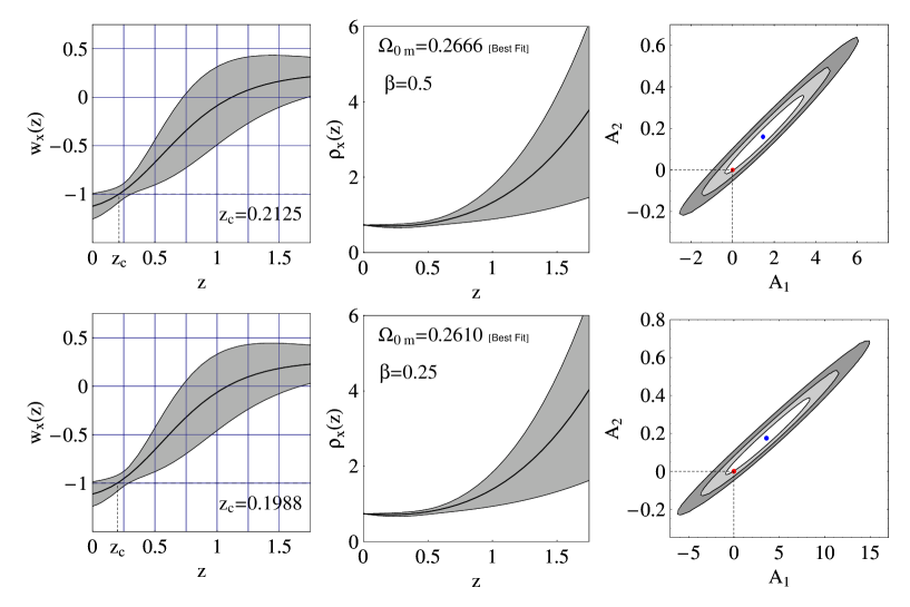
The evolution of and (in units of ), alongwith the corresponding errors, for , as well as the and contours are shown in Fig. 1, for both the choices and . One may also have the and contour plots for either choice, however for brevity we have suppressed those plots. The cases and are potentially not much distinct. The vs plots show that the value at which the best fit crosses is for and for . Both these values of are fairly in agreement with those obtained for popular model-independent ansatze for [13], [14], [15], [16], etc. The cosmological constant (corresponding to ), is found to be about away from the best fit result for both the choices and .
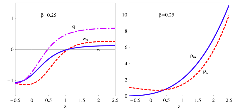
The left panel of Fig. 2 shows the variations of the DE EoS parameter , the total EoS parameter , Eq. (10), and the deceleration parameter , Eq. (11), for the best fit parameters , extrapolated to the red-shift range . The transition from the decelerating () phase to the accelerating () phase occurs at and the values of both and are greater than at present (). Whereas the present value of , there is a tendency that would turn back from a minimum value towards the cosmological constant value () in distant future (). Thus the phantom () phase may be transient, so that future singularities, such as the Big Rip, may be avoided. The right panel of Fig. 2 shows the variations of the matter density and the extrapolated best fit DE density (both in units of the present critical density ) with , for . The DE density is found to almost track the matter density for higher red-shifts, until equalling it at and dominant thereafter333For very high red-shifts () we find that extrapolated exceeds once again and the DE becomes more and more dominant as we go further and further in the past. However, the best fit model parameters, which give rise to such a variation of , are found by fitting the Union data available only up to . Therefore the extrapolation of to such high red-shifts, using these parametric values, cannot be trusted with much confidence after all.. Thus the model apparently resolves the coincidence problem, side by side providing a PDL crossing DE. The extrapolation of the best fit to future epochs also show that the DE density, though dominant, does not run away to very high values, causing Big Rip-like singularities. Both the plots of Fig. 2 correspond to the choice , for which the model fits better with the Union data, as mentioned above.
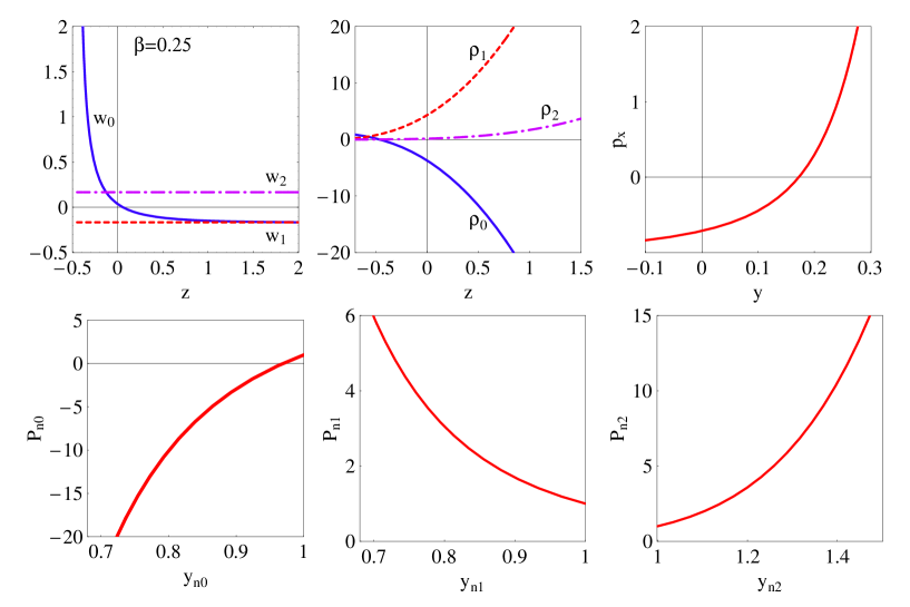
All the plots of Fig. 3 also correspond to the choice . The upper left panel of Fig. 3 shows the extrapolated best fit variations of the EoS parameters corresponding to the individual fields () with red-shift , for . While and are negative and positive constants equal in magnitude, the EoS parameter increases from a negative constant value (equal to ) in distant past, crosses zero in very recent past () and then goes on increasing with positive values. The upper middle panel of Fig. 3 shows the extrapolated best fit variations of the individual field energy densities with , for . and are positive definite and decreases with time (i.e., with decreasing ). is negative in the past and at present, but increases with time, and may become positive in distant future (), as the extrapolations show. In magnitude the value of is found to be very small compared to and for all the red-shift range shown in the figure. and , on the other hand, are nearly equal in magnitude for .
Now, the effective DE EoS parameter is given by
| (51) |
Since is always positive, the negative definite and positive definite contributors to are (for which ) and (for which ) respectively. The field , on the other hand, gives positive contribution () to right from the past up to and negative contribution () thereafter. However this field , though has a negative energy density (phantom-like), could not have led to the PDL crossing at , as its negative contribution to begins only after . It is therefore the (non-phantom-like) field , with positive definite energy density , which is effectively responsible for the PDL crossing at . This is in contrast with the usual quintom mechanism [25] where the negative energy density (phantom) field leads to the PDL crossing at late times. Moreover, none of the three fields above has EoS parameter less than , as in quintom models.
We reconstruct the multiple kinetic k-essence Lagrangian using the best fit values of the parameters for the choice . The parametric plot of against the total temporal field gradient , for red-shifts , in the upper right panel of Fig. 3 shows three separate phases: (i) for , whence the DE is decelerating (), (ii) for , whence the DE is accelerating but with , (iii) for , whence we have a super-accelerating (i.e., phantom-like) DE with . The parametric plots of the reconstructed normalized k-essence Lagrangian components (where ) against the corresponding normalized temporal field gradients (where ), for , are shown in the lower panels of Fig. 2. In the reconstructions, we have set for simplicity and appearing in Eqs. (27) and (34) to be zero, whence the cosmological constant term in Eq. (4.2) is given by . The pressure is found to fall off with increasing values of , whereas the pressures and are found to increase, but with opposite rates, with and respectively. Since the best fit values of both the parameters are positive, the only parameter with a negative value is (for ). Therefore, the fields which contribute to the negative part of are (due to the negative constant value of EoS parameter , but positive definite energy density ) and (due to the negative parameter , or , which drives and/or to be negative, in some regime). However, as explained above, the field alone is not responsible for the PDL crossing, and it is the field with Lagrangian component which effectively causes the super-acceleration ().
6 Conclusions
While a PDL crossing DE model involving a single k-essence scalar field suffers from cosmological instabilities [35], a set of multiple k-essence fields are shown to give rise to such PDL crossing, satisfying the conditions for stability even in the simplistic scenario where the k-fields are mutually non-interacting and the individual k-essence Lagrangian densities are purely functions of the kinetic terms. Although there are severe restrictions imposed on the k-field configuration by virtue of the stability criterion, i.e., , and the non-super-luminescence () of the DE density perturbations, we still find certain field configurations for which the DE EoS parameter can cross the cosmological constant barrier. We have worked out the general equation of constraint on the field configuration, with an appropriate choice of the propagation speed, viz., a constant, lying between and . While a configuration of two kinetic k-fields, satisfying the constraint equation, leads to complicated solutions, we have shown that a three k-field configuration gives rise to a cosmologically stable PDL crossing DE model. For certain choices of some of the parameters, the model is found to fit well with the latest SNIa Union data compiled by the Supernova Cosmology Project team [7]. The value of the red-shift at which the DE equation of state parameter (best fit with the data) crosses the PDL is found to be , whereas the best fit present matter density parameter is found to be . These are in good agreement with the values of and found in the likelihood analysis done using other model-dependent or model-independent ansatze in the literature [16, 17, 49]. On the other hand, the value of at which the universe transits from a decelerating phase to an accelerating phase is found to be , which also agrees fairly well with other independent studies [16, 17, 49].
In the model which we have presented here, the value of the square of the speed of propagation of the DE density perturbations, , is as low as throughout the entire course of the DE evolution. We have worked out the expression for in a general setting of multiple k-essence fields considering the most general scalar type of metric perturbations in a Friedmann-Robertson-Walker background. Although the perturbation equations have been extremely coupled in the curvature and the isocurvature modes, assuming the coupling to be very weak in the sub-Hubble scales the speed of propagation of the curvature perturbations in the multi-k-field case is found to be the one that generalizes the well-known expression for for a single k-essence field found in ref. [45].
The present model exhibits some additional features: Firstly, the dark energy density (best fit with the Union data) almost tracks the matter density in distant past until exceeding the later at , thus providing a possible resolution to the coincidence problem. Secondly, the best fit dark energy density, extrapolated to future epochs, does not run away to very high values leading to Big Rip-like singularities even in distant future. Thirdly, the extrapolated best fit of the dark energy equation of state parameter shows a tendency to turn back from a minimum negative value () towards the cosmological constant value () in distant future, thus indicating a transient phantom regime.
We have reconstructed the entire k-essence Lagrangian , as well as the individual Lagrangian components in terms of the corresponding field gradients , using the values of the model parameters best fitting the observational data. The reconstructed total Lagrangian, is found to be a smooth function of the total field gradient , i.e., there are no discontinuities or multi-valuedness in the parametric plot of versus for the red-shift range under consideration, . All the individual Lagrangian components as functions of the corresponding also show the same smooth nature. The reconstructed Lagrangian is therefore substantially better than the double-valued Lagrangian found for a single kinetic k-essence field in ref. [52] using popular parameterizations, such as that due to Alam et al [14] or due to Chevallier-Polarski-Linder [13] and with the old SNIa gold data-set [3].
A few problems that may be looked upon in the context of the present model are as follows: (i) Can we find a systematic prescription in order to build a stable PDL crossing multiple kinetic k-essence model, instead of choosing the number of k-fields by hand and implementing the value of arbitrarily? (ii) Can we extend the model to sufficiently higher red-shifts so as to match with the CMB and SDSS data? (iii) Is there a way to ascertain how far the isocurvature modes of the density perturbations affect the model at higher red-shifts? (iv) Can we ascertain the status of the future Big Rip singularities, if any, in the context of multi-k-essence, generically, i.e., by not just resorting to particular models? Or, can we generically ascertain whether the phantom regime would be eternal or transient for multiple k-essence? Research works addressing some of these questions are already in progress [46] and we hope to report on them in near future.
Finally, it should be mentioned that although we have not specifically looked to construct tracking/scaling dark energy models in the present paper, the possible avoidance of the coincidence problem in our multi-k-essence model is particularly noteworthy. The value of remains constant and less than the speed of light, unlike in the coincidence resolving single field k-essence models, which are shown to be affected by the super-luminal propagation () of the density perturbations [47]. However, whether our purely kinetic model specifically belongs to the class of tracking or scaling k-essence dark energy, is an interesting issue which we hope to circumvent in future. Assisted accelerated solutions are shown to exist generically for the multi-field k-essence models that have scaling solutions [53]. The nature of such assisted acceleration may also be of some interest for the purely kinetic multi-k-essence, that we have studied here, and is worth investigating.
Appendix: Speed of propagation of multiple k-essence cosmological perturbations
Let us consider the system of mutually non-interacting k-essence fields coupled to gravity. The gravitational field equations for such a system are
| (52) |
where are the energy-momentum tensor components due to the individual k-fields , with kinetic terms , where .
The line element with the most general scalar type of perturbations, in an arbitrary gauge, is given by [54]:
| (53) | |||||
where is the cosmological scale factor, and and are the perturbed order variables. The perturbed energy-momentum tensor components are given by
| (54) |
where and are the total background energy density and isotropic pressure respectively, and are the perturbed total energy density and isotropic pressure respectively, is the velocity (or, flux) related variable, is the anisotropic stress, and is the co-moving wave-number. Decomposing into the components due to individual k-fields, we have
| (55) |
The background field equations are the Friedmann equations and the equations of continuity of the individual scalar fields:
| (56) | |||
| (57) | |||
| (58) |
The equations for the cosmological perturbations
| (59) |
can be decomposed as
| (60) | |||||
| (61) | |||||
| (62) | |||||
| (63) |
where
| (64) |
and note that for a scalar field system in RW background. The quantities and correspond respectively to the three-space curvature, the shear, and the perturbed expansion of the normal-frame vector field [39, 40]. Eq. (60) gives the Arnowitt-Deser-Misner (ADM) energy constraint, Eq. (61) gives the momentum constraint, Eq. (62) is the trace-free part of the ADM propagation, and Eq. (63) is the Raychaudhuri equation [40]. In addition to the above equations, we have the energy and momentum conservation equations given by
| (65) | |||||
| (66) |
The entropic perturbations are given by
| (67) |
where and .
Under a coordinate transformation
| (68) |
the metric perturbations transform as
| (69) |
whereas the field perturbations transform as
| (70) |
Since we are always free to choose and , we can impose two gauge conditions on the functions or or . We choose to work in the commonly used longitudinal gauge in which . Then from Eq. (64) , whence Eq. (62) gives , and the expression for in Eq. (64) reduces to
| (71) |
Curvature Perturbations:
The so-called gauge-invariant co-moving curvature perturbation variable is given by [55]
| (72) |
From Eqs. (60), (61), (67) and (71), one derives the equations for the curvature perturbations as
| (73) | |||
| (74) |
where the gauge invariant variable is defined by
| (75) |
Isocurvature Perturbations:
The total entropic perturbation can be decomposed as [40, 41]
| (76) |
where , and the so-called gauge-invariant isocurvature perturbation variable is defined as
| (77) |
From Eqs. (65), (66) and (67) one obtains the equations for the isocurvature perturbations
| (78) | |||||
| (79) | |||||
where .
Eqs. (73), (74) and (78), (79) form an extremely coupled set of differential equations in the curvature and isocurvature modes, very difficult to solve in general for any system of multiple fields. However, leaving aside the isocurvature terms, one may still work out the effective speed of propagation of curvature perturbations in such a system. In fact, in the large scale limit (), the curvature mode couples very weakly to the isocurvature ones, as is evident from the term on the right hand side of Eq. (79). For a detailed discussion on the issue of decoupling of isocurvature and curvature modes in multiple fluid or field systems, see ref. [40].
Now, in the case of mutually non-interacting multiple k-essence scalar fields, we have the expressions for the total energy density and pressure
| (80) | |||||
| (81) |
Using the continuity equations for the fields , and the fact that in RW background, we obtain the expressions for the perturbed variables and as
| (82) | |||||
| (83) |
where we have defined and .
The expressions for and , obtained from the components of the energy-momentum tensors, are given by
| (84) |
Defining further and , we get from Eqs. (72), (73) and (75)
| (85) | |||
| (86) | |||
| (87) |
where is the total number of fields and for the reasons mentioned earlier we have left aside the terms depending only on (and/or its time derivatives), which give rise to the isocurvature modes.
The equation (73) for the curvature mode can now be expressed as
| (88) |
where
| (89) |
is the effective speed of propagation of the curvature mode of scalar perturbations [46]. For a single k-field (), Eq. (89) reduces to the well-known result [45], whereas for purely kinetic multiple k-essence fields, we have , whence . If any of the fields is non-propagating, i.e., for some value of , then .
References
References
- [1] S. J. Perlmutter et al, Bull. Am. Astron. Soc. 29 1351 (1997); A. G. Riess et al, Astron. J. 116 1009 (1998); S. J. Perlmutter et al, Astrphys. J. 517 565 (1999).
- [2] J. L. Tonry et al, Astrophys. J. 594 1 (2003); R. Knop et al, Astrophys. J. 598 102 (2003); B. Baris et al, Astrophys. J. 602 571 (2004).
- [3] A. G. Riess et al, Astrophys. J. 607 665 (2004).
- [4] A. G. Riess et al, Astrophys. J. 659 98 (2007).
- [5] P. Astier et al, Astron. Astrophys. 447 31 (2006).
- [6] T. M. Davis et al, Astrophys. J. 666 716 (2007); G. Miknaitis et al, Astrophys. J. 666 674 (2007); W. M. Wood-Vasey et al, Astrophys. J. 666 694 (2007);
- [7] M. Kowalski et al, arXiv:0804.4142 [astro-ph].
- [8] D. Rubin et al, arXiv:0807.1108 [astro-ph].
- [9] D. N. Spergel et al, Astrophys. J. Suppl. 148 175 (2003); C. L. Bennet et al, Astrophys. J. Suppl. 148 1 (2003).
- [10] D. N. Spergel et al, Astrophys. J. Suppl. 170 377 (2007); J. Dunkley et al arXiv:0803.0586 [astro-ph]; R. Hill et al arXiv:0803.0570 [astro-ph].
- [11] M. Tegmark et al, Phys. Rev. D74 123507 (2006); D. Eisenstein et al, Astrophys. J. 633 560 (2005).
- [12] S. M. Carroll, Living Rev. Rel. 4 1 (2001); T. Padmanabhan, Phys. Rept. 380 235 (2006), J. M. Cline, arXiv:hep-th/0612129; J. Polchinski, arXiv:hep-th/0603249; L. M. Krauss and R. J. Scherrer, Gen. Rel. Grav. 39 1545 (2007).
- [13] M. Chevallier and D. Polarski, Int. J. Mod. Phys. D10 213 (2001); E. V. Linder, Phys. Rev. Lett. 90 091301 (2003).
- [14] U. Alam, V. Sahni, T. D. Saini and A. A. Starobinsky, Mon. Not. Roy. Astron. Soc. 354 275 (2004).
- [15] M. Visser, CLass. Quant. Grav. 21 2603 (2004); A. A. Sen, Phys. Rev. D77 043508 (2008).
- [16] Y. G. Gong and A. Wang, Phys. Rev. D75 043520 (2007).
- [17] C. A. Shapiro and M. S. Turner, Astrophys. J. 649 563 (2006); H. K. Jassal, J. S. Bagla and T. Padmanabhan, Mon. Not. Roy. Astron.Soc. 356 L11 (2005); T. R. Choudhury and T. Padmanabhan, Astron. Astrophys. 429 807 (2005); E. V. Linder and D. Huterer, Phys. Rev. D72 043509 (2005); C. Wetterich, Phys. Lett. B594, 17 (2004); E. V. Linder, arXiv:0708.0024 [astro-ph]; F. C. Carvalho et al, Phys. Rev. Lett. 97 081301 (2006); J. S. Alcaniz and J. A. S. Lima, Phys. Rev. D72 063516 (2005); R. G. Cai and A. Wang, JCAP 0503 002 (2005).
- [18] T. Padmanabhan, Gen. Rel. Grav. 40 529 (2008); E. J. Copeland, M. Sami and S. Tsujikawa, Int. J. Mod. Phys. D15 1753 (2006); P. J. E. Peebles and B. Ratra, Rev. Mod. Phys. 75 559 (2003); V. Sahni and A. A. Starobinsky, Int. J. Mod. Phys. D9 373 (2000).
- [19] R. R. Caldwell, R. Dave and P. J. Steinhardt, Phys. Rev. Lett 80 1582 (1998); S. M. Carroll, Phys. Rev. Lett. 81 3067 (1998); E. J. Copeland, A. R. Liddle and D. Wands, Phys. Rev. D57 4686 (1998); P. J. Steinhardt, L. M. Wang and I. Zlatev, Phys. Rev. D59 123504 (1999); I. Zlatev, L. M. Wang and P. J. Steinhardt, Phys. Rev. Lett. 82 896 (1999); A. R. Liddle and R. J. Scherrer, Phys. Rev. D59 023509 (1999).
- [20] R. R. Caldwell, Phys. Lett. B545 23 (2002); N. Arkani-Hamed, P. Creminelli, S. Mukohyama and M. Zaldarriaga, JCAP 0404 001 (2004); F. Piazza and S. Tsujikawa, JCAP 0407 004 (2004); L. P. Chimento and R. Lazkoz, Phys. Rev. Lett. 91 211301 (2003); S. Tsujikawa, Class. Quant. Grav. 20 1991 (2003); L. Perivolaropoulos, Phys. Rev. D71 063503 (2005); S. Nesseris and L. Perivolaropoulos, Phys. Rev. D70 123529 (2004).
- [21] S. M. Carroll, M. Hoffman and M. Trodden, Phys. Rev. D68 023509 (2003).
- [22] J. M. Cline, S. Y. Jeon and G. D. Moore, Phys. Rev. D70 043543 (2004).
- [23] R. R. Caldwell, M. Kamionkowski and N. N. Weinberg, Phys. Rev. Lett. 91 071301 (2003).
- [24] S. Nojiri, S. D. Odintsov and S. Tsujikawa, Phys. Rev. D71 063004 (2005).
- [25] B. Feng, X. L. Wang and X. M Zhang, Phys. Lett. B607 35 (2005); Z. K. Guo, Y. S. Piao, X. M. Zhang and Y. Z. Zhang, Phys. Lett. B608 177 (2005); B. Feng, M. Li, Y. S. Piao and X. Zhang, Phys. Lett. B634 101 (2006); R. Lazkoz and G. Leon, Phys. Lett. B638 303 (2006); R. Lazkoz, G. Leon and I. Quiros, Phys. Lett. B649 103 (2007); Y. Cai, M. Li, J. X. Lu, Y. S. Piao, T. Qiu and X. Zhang, Phys. Lett. B651 1 (2007); Y. Cai, H. Li, Y. S. Piao, X. Zhang, Phys. Lett. B646 141 (2007).
- [26] B. Boisseau, G. Esposito-Farese, D. Polarski and A. A. Starobinsky, Phys. Rev. Lett. 85 2236 (2000); G. Esposito-Farese and D. Polarski, Phys. Rev. D63 063504 (2001); L. Perivolaropoulos, JCAP 0510 001 (2005); S. Nesseris and L. Perivolaropoulos, Phys. Rev. D73 103511 (2006).
- [27] V. Sahni and Y. Shtanov, JCAP 0311 014 (2003); V. Sahni and Y. Shtanov, Phys. Rev. D71 084018 (2005).
- [28] N. Arkani-Hamed, P. Creminelli, S. Mukohyama and M. Zaldariagga, JCAP 0404 001 (2004); F. Piazza and S. Tsujikawa, JCAP 0407 004 (2004).
- [29] V. K. Onemli and R. P. Woodard, Class. Quant. Grav. 19 4607 (2002); V. K. Onemli and R. P. Woodard, Phys. Rev. D70 107301 (2004); E. O. Kahya and V. K. Onemli, Phys. Rev. D76 043512 (2007).
- [30] B. Gumjudpai, T. Naskar, M. Sami and S. Tsujikawa, JCAP 0506 007 (2005).
- [31] See for example, L. Amendola and S. Tsujikawa, Phys. Lett. B660 125 (2008); and references therein.
- [32] H. Wei, R. G. Cai and D. F. Zeng, Class. Quant. Grav. 22 3189 (2005); H. Wei and R. G. Cai, Phys. Rev. D72 123507 (2005); H. Wei, N. N. Tang and S. N. Zhang, Phys. Rev. D75 043009 (2007).
- [33] C. Armendariz-Picon, V. F. Mukhanov and P. J. Steinhardt, Phys. Rev. Lett. 85 4438 (2000); C. Armendariz-Picon, V. F. Mukhanov and P. J. Steinhardt, Phys. Rev. D63 103510 (2001); C. Armendariz-Picon, T. Damour and V. F. Mukhanov, Phys. Lett. B458 209 (1999); T. Chiba, T. Okabe and M. Yamaguchi, Phys. Rev. D62 023511 (2000).
- [34] M. Malquarti, E. J. Copeland, A. R. Liddle and M. Trodden, Phys. Rev. D67 123503 (2003); M. Malquarti, E. J. Copeland and A. R. Liddle, Phys. Rev. D68 023512 (2003); J. M. Aguirregabiria, L. P. Chimento and R. Lazkoz, Phys. Rev. D70 023509 (2004); L. P. Chimento and A. Feinstein, Mod. Phys. Lett. A19 761 (2004); L. P. Chimento, Phys. Rev. D69 123517 (2004).
- [35] A. Vikman, Phys. Rev. D71 023515 (2005).
- [36] S. Capozziello, S. Nojiri and S. D. Odintsov, Phys. Lett. B632 597 (2006); S. Nojiri and S. D. Odintsov, Gen. Rel. Grav. 38 1285 (2006).
- [37] A. A. Andrianov, F. Cannata and A. Y. Kamenshchik, Phys. Rev. D72 043531 (2005); F. Cannata and A. Y. Kamenshchik, Int. J. Mod. Phys. D16 1683 (2007); A. K. Sanyal, arXiv:0710.3486 [astro-ph].
- [38] L. P. Chimento and R. Lazkoz, Phys. Lett. B639 591 (2006).
- [39] J. Hwang, Astrophys. J. 375 443 (1991).
- [40] J. Hwang and H. Noh, Class. Quant. Grav. 19 527 (2002); J. Hwang and H. Noh, Phys. Lett. B495 277 (2000).
- [41] H. Kodama and M. Sasaki, Prog. Theor. Phys. Suppl. 78 1 (1984); H. Kodama and M. Sasaki, Int. J. Mod. Phys. A1 265 (1986); ibid A2 491 (1987).
- [42] C. Gordon, D. Wands, B. A. Bassett and R. Maartens, Phys. Rev. D63 023506 (2001).
- [43] D. Langlois and S. Renaux-Petel, JCAP 0804 017 (2008); D. Langlois, S. Renaux-Petel, D. A. Steer and T. Tanaka, 0806.0336 [hep-th]; X. Gao, JCAP 0806 029 (2008).
- [44] F. Arroja, S. Mizuno and K. Koyama, JCAP 0808 015 (2008); D. Langlois, S. Renaux-Petel, D. A. Steer and T. Tanaka, Phys. Rev. Lett. 101 061301 (2008); M. Huang, G. Shiu and B. Underwood, Phys. Rev. D77 023511 (2008); D. A. Easson, R. Gregory, D. F. Mota, G. Tasinato and I. Zavala, JCAP 0802 010 (2008).
- [45] J. Garriga and V. F. Mukhanov, Phys. Lett. B458 219 (1999).
- [46] S. Sur, in preparation.
- [47] C. Bonvin, C. Caprini and R. Durrer, Phys. Rev. Lett. 97 081303 (2006) [arXiv:astro-ph/0606584].
- [48] E. Babichev, V. F. Mukhanov and A. Vikman, JHEP 0802 101 (2008); E. Babichev, V. F. Mukhanov and A. Vikman, JHEP 0609 061 (2006); J. Bruneton, Phys. Rev. D75 085013 (2007); J. Bruneton and G. Esposito-Farese, Phys. Rev. D76 124012 (2007).
- [49] S. Nesseris and L. Perivolaropoulos, JCAP 0701 018 (2007); S. Nesseris and L. Perivolaropoulos, Phys. Rev. D72 123519 (2005); V. Sahni and A. A. Starobinsky, Int. J. Mod. Phys. D15 2105 (2006); U. Alam, V. Sahni and A. A. Starobinsky, JCAP 0702 011 (2007); L. P. Chimento, R. Lazkoz, R. Maartens and I. Quiros, JCAP 0609 004 (2006); S. Fay and R. Tavakol, arXiv:0801.2128 [astro-ph].
- [50] S. Sur and S. Das, in preparation.
- [51] L. Perivolaropoulos, Phys. Rev. D71 063503 (2005); E. Di Pietro and J. F. Claeskens, Mon. Not. Roy. Astron.Soc. 341 1299 (2003).
- [52] A. A. Sen, JCAP 0603 010 (2006).
- [53] S. Tsujikawa, Phys. Rev. D73 103504 (2006) [arXiv:hep-th/0601178].
- [54] J. M. Bardeen, Phys. Rev. D22 1882 (1980); V. F. Mukhanov, H. A. Feldman and R. H. Brandenberger, Phys. Rept. 215 203 (1992); V. F. Mukhanov, Physical Foundations of Cosmology, Cambridge Univ. Press, Cambridge, UK (2005).
- [55] J. Hwang and E. T. Vishniac, Astrophys. J. 353 1 (1990); G. V. Chibisov and V. F. Mukhanov, Mon. Not. Roy. Astron. Soc. 200 535 (1982); V. N. Lukash, Sov. Phys. - JETP Lett. 31 596 (1980); V. N. Lukash, Sov. Phys. - JETP 52 807 (1980).