Density probability distribution functions of diffuse gas in the Milky Way

Abstract

In a search for the signature of turbulence in the diffuse interstellar medium in gas density distributions, we determined the probability distribution functions (PDFs) of the average volume densities of the diffuse gas. The densities were derived from dispersion measures and $\mathrm{H\,\scriptstyle I}$ column densities towards pulsars and stars at known distances. The PDFs of the average densities of the diffuse ionized gas (DIG) and the diffuse atomic gas are close to lognormal, especially when lines of sight at $|b|<5^{\circ}$ and $|b|\geq 5^{\circ}$ are considered separately. The PDF of $\langle\,n_{\mathrm{H\,\scriptstyle I}}\,\rangle$ at high $|b|$ is twice as wide as that at low $|b|$. The width of the PDF of the DIG is about $30$ per cent smaller than that of the warm $\mathrm{H\,\scriptstyle I}$ at the same latitudes. The results reported here provide strong support for the existence of a lognormal density PDF in the diffuse ISM, consistent with a turbulent origin of density structure in the diffuse gas.

1 Introduction

Simulations of the interstellar medium (ISM) have shown that, if isothermal turbulence is shaping the structure of the medium, the density distribution becomes lognormal (Elmegreen & Scalo, 2004, and references therein). However, Madsen et al. (2006) found large temperature differences between lines of sight through the warm ionized medium, which seem inconsistent with an isothermal gas. Also in the MHD simulations of de Avillez & Breitschwerdt (2005) and Wada & Norman (2007) the ISM became non-isothermal. The latter authors showed that for a large enough volume, and for a long enough simulation run, the physical processes causing the density variations in the ISM in a galactic disc can be regarded as random and independent events. Therefore, the PDF of log(density) becomes Gaussian and the density PDF lognormal, although the medium is not isothermal. The medium is inhomogeneous on a local scale, but in a quasi-steady state on a global scale.

The shape of the gas density PDF can be an important component in theories of star formation. Elmegreen (2002) showed that a Schmidt-type power-law relation between the star formation rate per unit area and the gas surface density can be deduced if the density PDF is lognormal and star formation occurs above a threshold density: the dispersion of the lognormal density PDF is a key parameter in the model. However, from the existing simulations it is not yet clear whether a lognormal density PDF in galaxies is universal and which factors determine their shape (Wada & Norman, 2007).

Little observational evidence exists to test the results of the simulations. Wada et al. (2000) showed that the luminosity function of the HI column density in the Large Magellanic Cloud is lognormal. Recently, Hill et al. (2007, 2008) derived a lognormal distribution of the emission measures perpendicular to the Galactic plane of the DIG in the Milky Way, observed in the Wisconsin H$\alpha$ Mapper survey (Haffner et al., 2003) above Galactic latitudes of $10^{\circ}$. They note that emission measures towards classical HII regions also fit a lognormal distribution, with different parameters. Furthermore, Tabatabaei (2008) found a lognormal distribution of the emission measures derived from an extinction-corrected H-$\alpha$ map of the nearby galaxy M33 (Tabatabaei et al., 2007). Gaustad & Van Buren (1993) plotted the distribution of the local volume density of dust near stars within 400$\,\mathrm{pc}$ of the Sun, which is also consistent with a lognormal distribution. In this Letter we present the PDFs of average volume densities of the DIG and the diffuse atomic gas in the Milky Way, and show that they are consistent with lognormal distributions as well.

2 Basics and Data

We investigated the density PDFs of the DIG and of diffuse atomic hydrogen gas ($\mathrm{H\,\scriptstyle I}$) in the solar neighbourhood.

Various volume densities of the DIG can be obtained from the dispersion measure $\,\mathrm{DM}$ (in $\,\mathrm{cm^{-3}}\,\mathrm{pc}$) and emission measure $\,\mathrm{EM}$ (in $\mathrm{cm}^{-6}\,\mathrm{pc}$) towards a pulsar at known distance $D$ (in $\,\mathrm{pc}$) from the relations:

$$\,\mathrm{DM}=\int_{0}^{D}\,n_{\mathrm{e}}(l)\,\mathrm{d}l=\langle\,n_{\mathrm{e}}\,\rangle\,D=\,N_{\mathrm{c}}\,F_{\mathrm{d}}\,D,$$ (1)

$$\,\mathrm{EM}=\int_{0}^{D}\,n_{\mathrm{e}}^{2}(l)\,\mathrm{d}l=\langle\,n_{\mathrm{e}}^{2}\,\rangle\,D=\,N_{\mathrm{c}}^{2}\,F_{\mathrm{d}}\,D,$$ (2)

where $\,n_{\mathrm{e}}(l)$ is the local electron density at point $l$ along the line-of-sight (LOS), $\langle\,n_{\mathrm{e}}\,\rangle$ and $\langle\,n_{\mathrm{e}}^{2}\,\rangle$ are averages along $D$ and $\,F_{\mathrm{d}}$ is the fraction of the line of sight in clouds of average density $\,N_{\mathrm{c}}$ (see fig. 1 in Berkhuijsen et al., 2006). The final equality in Eq. 2 is only valid when the average density of every cloud $n_{c}$ along the LOS is the same: then $\langle\,n_{\mathrm{e}}^{2}\,\rangle=\langle n_{c}^{2}\,\rangle\,F_{\mathrm{d}}=\,N_{\mathrm{c}}^{2}\,F_{\mathrm{d}}$. Thus $\,N_{\mathrm{c}}$ and $\,F_{\mathrm{d}}$ are crude approximations of the true average cloud density and filling factor along a LOS, but given the large number of different LOS in our sample their mean and dispersion are reasonable estimators of $\,N_{\mathrm{c}}$ and$\,F_{\mathrm{d}}$.

Combining Equations (1) and (2) we have

$$\,N_{\mathrm{c}}=\frac{\,\mathrm{EM}}{\,\mathrm{DM}},$$ (3)

and

$$\,F_{\mathrm{d}}=\frac{\,\mathrm{DM}^{2}}{\,\mathrm{EM}\ D}=\frac{\langle\,n_{\mathrm{e}}\,\rangle}{\,N_{\mathrm{c}}}.$$ (4)

The line-of-sight filling factor $\,F_{\mathrm{d}}$ approximates the volume filling factor $\,F_{\mathrm{v}}$ if there are several clouds along the line of sight. As this will generally be the case, we take $\,F_{\mathrm{v}}=\,F_{\mathrm{d}}$.

We used the densities derived from two pulsar samples that were originally selected for studies of the volume filling factor of the DIG.

1. 34 pulsars at observed distances known to better than $50$ per cent, collected by Berkhuijsen & Müller (2008). The pulsar distances are in the range $0.1<D<9.5\,\mathrm{kpc}$, with a mean distance of $2.4\,\mathrm{kpc}$ and a standard deviation of $2.9\,\mathrm{kpc}$ (the spread is large because 21 pulsars lie at $D<2\,\mathrm{kpc}$).

2. 157 pulsars with distances obtained from DM and the model of the distribution of free electrons in the MW of Cordes & Lazio (2002), collected by Berkhuijsen et al. (2006). These pulsars lie in the range $0.1<D<6\,\mathrm{kpc}$, with mean distance $1.7\,\mathrm{kpc}$ and standard deviation $1.0\,\mathrm{kpc}$.

Apart from 6 pulsars in the small sample, all pulsars are located at $|b|\geq 5^{\circ}$ in order to ensure that the lines of sight towards the pulsars probe the DIG and not denser $\mathrm{H\,\scriptstyle II}$ regions. The dispersion measures were taken from the catalogue of Manchester et al. (2005). The emission measures in the direction of the pulsars were obtained from H$\alpha$ surveys (Haffner et al., 2003; Finkbeiner et al., 2002) and corrected for extinction (Diplas & Savage, 1994b; Dickinson et al., 2003) as well as for H$\alpha$ emission originating beyond the pulsars. We refer to the work of Berkhuijsen et al. (2006, hereafter called BMM) and Berkhuijsen & Müller (2008) for further details.

Diplas & Savage (1994b) studied the scale height of the diffuse dust and the diffuse atomic gas using 393 stars in the Galaxy. We calculated the average $\mathrm{H\,\scriptstyle I}$ volume density, $\langle\,n_{\mathrm{H\,\scriptstyle I}}\,\rangle$ (in $\,\mathrm{cm^{-3}}$), from the column density $\,N(\mathrm{H\,\scriptstyle I})$ (in $\mathrm{cm}^{-2}$), corrected for contributions from the star, and the distance to the star as given in Table 1 of Diplas & Savage (1994a):

$$\,N(\mathrm{H\,\scriptstyle I})=\int_{0}^{D}\,n_{\mathrm{H\,\scriptstyle I}}(l)\,\mathrm{d}l=\langle\,n_{\mathrm{H\,\scriptstyle I}}\,\rangle\,D,$$ (5)

where $\,n_{\mathrm{H\,\scriptstyle I}}(l)$ (in $\,\mathrm{cm^{-3}}$) is the local volume density at distance $l$ along the line of sight. We removed 18 stars from the sample with denser clouds in their lines of sight indicated in Fig. 9 of Diplas & Savage (1994b), leaving the data towards 375 stars for analysis. The stars in this sample have distances in the range $0.1<D<11\,\mathrm{kpc}$, with a mean distance of $2.2\,\mathrm{kpc}$ and standard deviation $1.7\,\mathrm{kpc}$.

3 Results

3.1 Density PDFs of the DIG

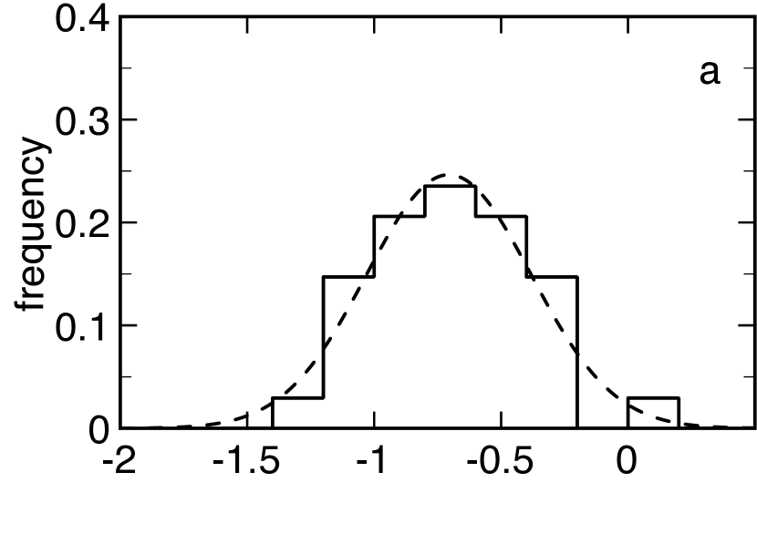
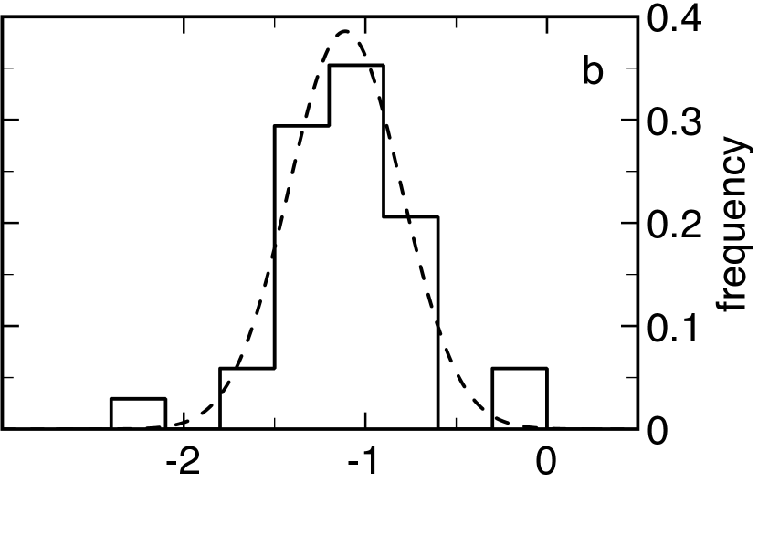
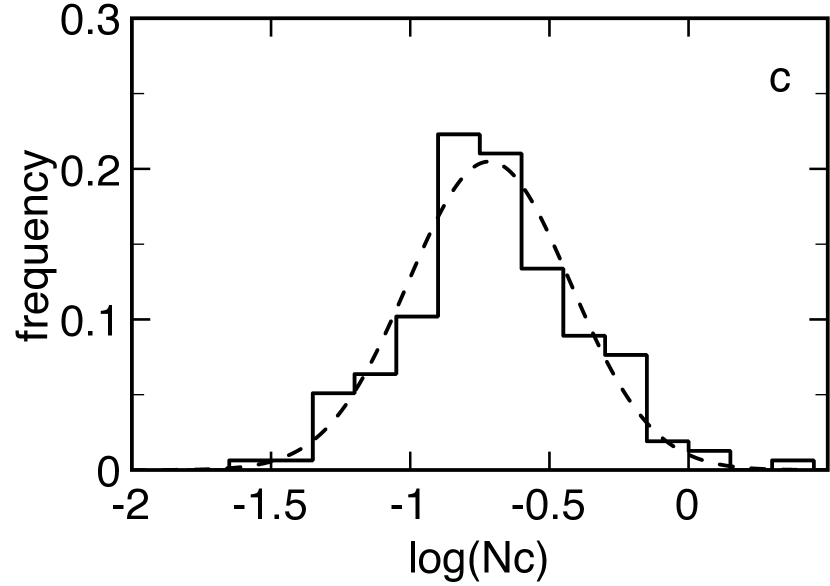
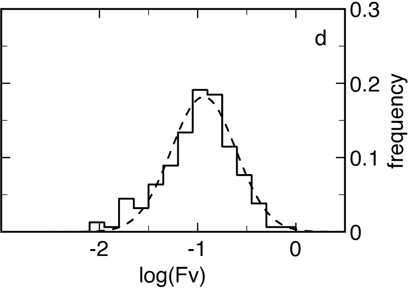
Figure 1: Probability distribution functions of mean density in clouds, $\,N_{\mathrm{c}}$ (a and c) and volume filling factors, $\,F_{\mathrm{v}}$ (b and d). The dashed lines are the lognormal fits to the histograms; the fit parameters are given in Table 1. Top: small sample (34 pulsars); bottom: BMM sample (157 pulsars).

Table 1: Lognormal fits to the PDFs of the DIG (Figs. 1 and 2). The fitted function is $Y=(\sqrt{2\pi}\sigma)^{-1}\exp[-(\log_{10}X-\mu)^{2}/2\sigma^{2}]$.

		Position of maximum		Dispersion
Sample	$X$	$\mu$	$X$	$\sigma$	$\chi^{2}$
This work	$\,N_{\mathrm{c}}$ ($\,\mathrm{cm^{-3}}$)	$-0.71\pm 0.03$	$0.19\pm 0.02$	$0.32\pm 0.03$	$0.4$
$N=34$	$\,F_{\mathrm{v}}$	$-1.11\pm 0.03$	$0.078\pm 0.006$	$0.31\pm 0.03$	$0.8$
	$\langle\,n_{\mathrm{e}}\,\rangle$ ($\,\mathrm{cm^{-3}}$)	$-1.83\pm 0.02$	$0.015\pm 0.001$	$0.22\pm 0.02$	$0.3$
	$\langle\,n_{\mathrm{e}}^{2}\,\rangle$ ($\mathrm{cm}^{-6}$)	$-2.48\pm 0.02$	$0.0033\pm 0.0002$	$0.29\pm 0.02$	$0.4$
BMM	$\,N_{\mathrm{c}}$ ($\,\mathrm{cm^{-3}}$)	$-0.72\pm 0.02$	$0.19\pm 0.01$	$0.29\pm 0.02$	$1.7$
$N=157$	$\,F_{\mathrm{v}}$	$-0.94\pm 0.02$	$0.115\pm 0.005$	$0.33\pm 0.02$	$0.9$
	$\langle\,n_{\mathrm{e}}\,\rangle$ ($\,\mathrm{cm^{-3}}$)	$-1.68\pm 0.01$	$0.021\pm 0.001$	$0.12\pm 0.01$	$1.2$
	$\langle\,n_{\mathrm{e}}^{2}\,\rangle$ ($\mathrm{cm}^{-6}$)	$-2.41\pm 0.03$	$0.0039\pm 0.0003$	$0.34\pm 0.03$	$0.8$

$Y$ is the fraction of sightlines in each bin divided by the logarithmic bin-width $\,\mathrm{d}(\log_{10}X)$. $\chi^{2}$ is the reduced chi-squared goodness of fit parameter, with the error in each bin $\delta_{i}$ estimated as $\delta_{i}=\sqrt{N_{i}}$ and for (number of bins$-2$) degrees of freedom.

In Fig. 1a we present the probability distribution function (PDF) of the mean density in clouds, $\,N_{\mathrm{c}}$, for the sample of 34 pulsars. As the volume filling factor is (anti-) correlated with $\,N_{\mathrm{c}}$ (see BMM), we show the PDF of $\,F_{\mathrm{v}}$ for the same sample in Fig. 1b. In log space, both PDFs are consistent with a Gaussian distribution, which is equivalent to a lognormal distribution in linear space. The PDFs have about the same dispersion, $\sigma$ (see Table 1). The positions of the maxima, $\mu$ = log(density of maximum), correspond to $\,N_{\mathrm{c}}=0.19\pm 0.02\,\mathrm{cm^{-3}}$ and $\,F_{\mathrm{v}}=0.078\pm 0.006$, which represent the centre of gravity in the $\,F_{\mathrm{v}}$-$\,N_{\mathrm{c}}$ plot in fig.6 of Berkhuijsen & Müller (2008). This sample is rather small, with low counts $N_{i}$ in the histogram bins and (probably) overestimated Poisson errors $\delta_{i}=\sqrt{N_{i}}$ leading to rather small reduced-$\chi^{2}$ statistics (Table 1). Therefore we also calculated the PDFs of $\,N_{\mathrm{c}}$ and $\,F_{\mathrm{v}}$ for the much larger sample of BMM, which are shown in Figs. 1c,d. Both are well fitted by Gaussians of widths that are nearly identical to those of the small sample (see Table 1). The positions of the maxima are at $\,N_{\mathrm{c}}=0.19\pm 0.01\,\mathrm{cm^{-3}}$ and $\,F_{\mathrm{v}}=0.115\pm 0.005$, corresponding to the centre of gravity in the $\,F_{\mathrm{v}}$-$\,N_{\mathrm{c}}$ plot of BMM (their fig.11). The good agreement between the PDFs of the two samples indicates that the statistical results on $\,F_{\mathrm{v}}$ and $\,N_{\mathrm{c}}$ of BMM are not influenced by the model distances and statistical absorption corrections that they used.

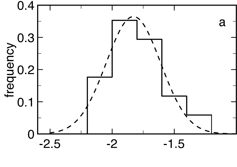
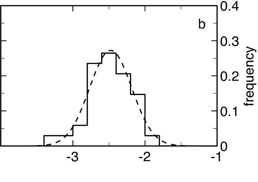
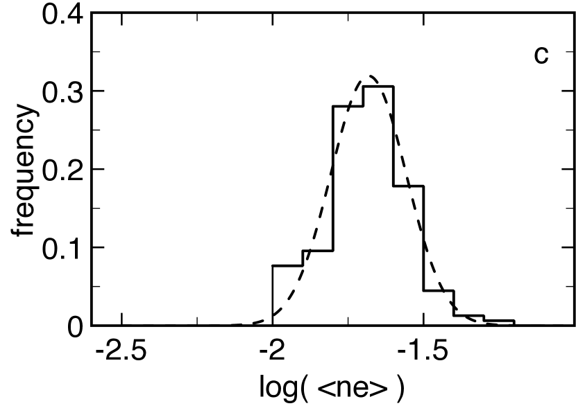
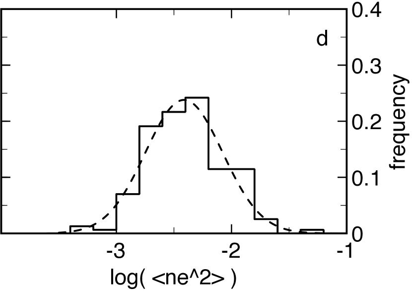
Figure 2: Probability distribution functions of $\langle\,n_{\mathrm{e}}\,\rangle=\,\mathrm{DM}/D$ (a and c) and $\langle\,n_{\mathrm{e}}^{2}\,\rangle=\,\mathrm{EM}/D$ (b and d) for the small sample (top) and the BMM sample (bottom). The dashed lines are the lognormal fits to the histograms; the fit parameters are given in Table 1.

In Fig. 2 we present the PDFs of the average densities $\langle\,n_{\mathrm{e}}\,\rangle$ and $\langle\,n_{\mathrm{e}}^{2}\,\rangle$ for both samples, all of which are well described by a lognormal distribution. The dispersion in $\langle\,n_{\mathrm{e}}\,\rangle$ is smaller than the dispersions in $\,F_{\mathrm{v}}$ and $\,N_{\mathrm{c}}$ due to their (anti-) correlation: $\,F_{\mathrm{v}}$ and $\,N_{\mathrm{c}}$ are not independent random variables. Note that the dispersion of the PDF of $\langle\,n_{\mathrm{e}}\,\rangle$ of the BMM sample is about half that of the small sample. As BMM used distances to the pulsars derived from the NE2001 model of Cordes & Lazio (2002), $\langle\,n_{\mathrm{e}}\,\rangle=\,\mathrm{DM}/D$ returns the densities of the model. The small dispersion reflects the fact that the model is much smoother than the density variations in the real ISM measured for the small sample. The dispersion in $\langle\,n_{\mathrm{e}}^{2}\,\rangle$ is larger than that of $\langle\,n_{\mathrm{e}}\,\rangle$ as the intrinsic spread in EM is much larger than in DM (see BMM; Berkhuijsen & Müller, 2008) while the distances used to calculate $\langle\,n_{\mathrm{e}}^{2}\,\rangle$ and $\langle\,n_{\mathrm{e}}\,\rangle$ are the same.

It is interesting to compare our data with the results of the magneto-hydrodynamic simulations of the ISM in the solar neighbourhood made by de Avillez & Breitschwerdt (2005). Their fig. 7 shows the density PDFs of five temperature regimes that developed after about $400\,\mathrm{Myr}$. The curve for $8000<T_{e}<16000\,\mathrm{K}$, which is most applicable to the DIG, closely resembles a lognormal with maximum at $\log(n_{H})=-0.75$ and dispersion $0.52$. The lognormal distribution extends over a much larger density range (at least $-2.5<\log(n_{H})<1.2$) than our observations of $\,N_{\mathrm{c}}$ ($-2<\log(\,N_{\mathrm{c}})<0$ in Fig. 1). The density of the maximum of $0.18\,\mathrm{cm^{-3}}$ agrees well with that of $\,N_{\mathrm{c}}=0.19\pm 0.02\,\mathrm{cm^{-3}}$ derived by us (see Table 1), but the dispersion is about $70$ per cent larger. This could be due to the larger temperature range of this component in de Avillez & Breitschwerdt (2005) compared to the $6000$-$10000\,\mathrm{K}$ observed for the DIG (Madsen et al., 2006).

We conclude that the PDFs of the electron densities and filling factors in the DIG in the solar neighbourhood are lognormal as is expected for a turbulent ISM from numerical simulations.

3.2 Density PDFs of diffuse $\mathrm{H\,\scriptstyle I}$

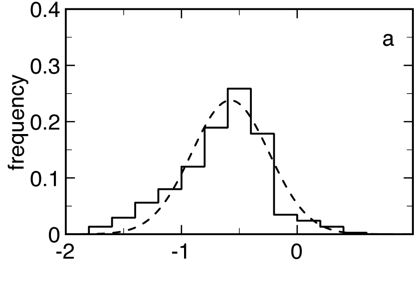
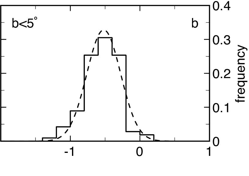
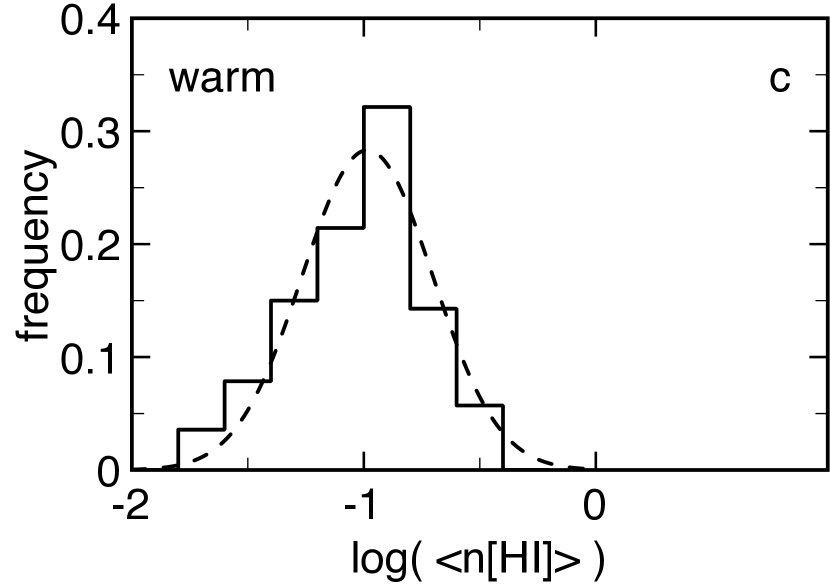
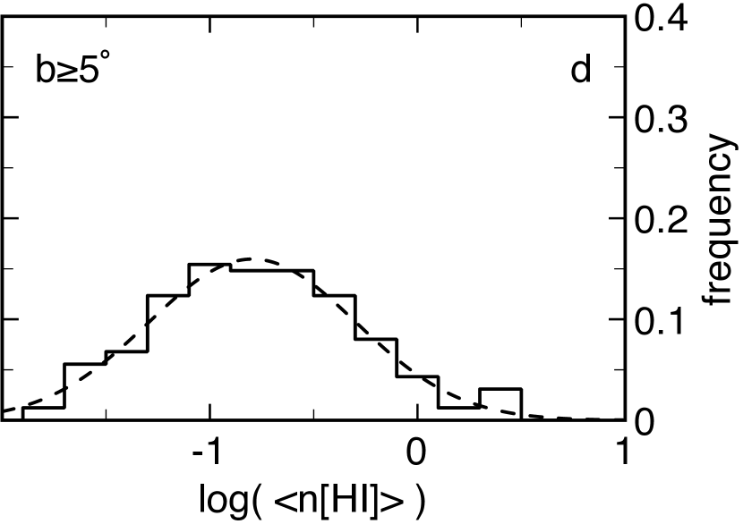
Figure 3: Probability distribution functions of $\langle\,n_{\mathrm{H\,\scriptstyle I}}\,\rangle=\,N(\mathrm{H\,\scriptstyle I})/D$: a) Full sample of 375 stars (Diplas & Savage, 1994a), of which are b) 213 stars at $|b|<5^{\circ}$ and d) 162 stars at $|b|\geq 5^{\circ}$; c) 140 stars seen through warm $\mathrm{H\,\scriptstyle I}$. The dashed lines are the lognormal fits to the histograms; the fit parameters are given in Table 2.

Table 2: Lognormal fits to the PDFs of $\langle\,n_{\mathrm{H\,\scriptstyle I}}\,\rangle$ (Fig. 3). The fitted function is $Y=(\sqrt{2\pi}\sigma)^{-1}\exp[-(\log_{10}\langle\,n_{\mathrm{H\,\scriptstyle I}}\,\rangle-\mu)^{2}/2\sigma^{2}]$.

		Position of maximum		Dispersion
Area	$N$	$\mu$	$\langle\,n_{\mathrm{H\,\scriptstyle I}}\,\rangle$	$\sigma$	$\chi^{2}$
All stars	$375$	$-0.57\pm 0.03$	$0.27\pm 0.02$	$0.34\pm 0.03$	$6.0$
$|b|<5^{\circ}$	$213$	$-0.52\pm 0.02$	$0.30\pm 0.02$	$0.24\pm 0.02$	$2.7$
$|b|\geq 5^{\circ}$	$162$	$-0.80\pm 0.02$	$0.16\pm 0.01$	$0.50\pm 0.02$	$0.4$
Warm $\mathrm{H\,\scriptstyle I}$	$140$	$-0.98\pm 0.03$	$0.10\pm 0.01$	$0.28\pm 0.03$	$2.5$
$|b|<5^{\circ}$	$42$	$-0.89\pm 0.01$	$0.13\pm 0.01$	$0.18\pm 0.01$	$0.1$
$|b|\geq 5^{\circ}$	$98$	$-1.07\pm 0.03$	$0.09\pm 0.01$	$0.33\pm 0.03$	$1.0$

$Y$ is the fraction of stars in each bin divided by the logarithmic bin-width $\,\mathrm{d}(\log_{10}\langle\,n_{\mathrm{H\,\scriptstyle I}}\,\rangle)$. $\chi^{2}$ is the reduced chi-squared goodness of fit parameter, with the error in each bin $\delta_{i}$ estimated as $\delta_{i}=\sqrt{N_{i}}$ and for (number of bins$-2$) degrees of freedom.

In Fig. 3a we present the PDF of the average volume density of $\mathrm{H\,\scriptstyle I}$, $\langle\,n_{\mathrm{H\,\scriptstyle I}}\,\rangle$, for the full sample of 375 stars of Diplas & Savage (1994a). Above $\mathrm{log}\langle\,n_{\mathrm{H\,\scriptstyle I}}\,\rangle=-1$ the distribution is approximately lognormal, but there is a clear excess at lower densities reflected in the large reduced-$\chi^{2}$ statistic (see Table 2). Because low densities can be expected away from the Galactic plane, we calculated the PDFs for the latitude ranges $|b|<5^{\circ}$ and $|b|\geq 5^{\circ}$ separately, as shown in Figs. 3b and 3d. Both distributions have a lognormal shape but they are shifted with respect to each other: the maximum of the low-$|b|$ sample is at $\langle\,n_{\mathrm{H\,\scriptstyle I}}\,\rangle=0.30\pm 0.02\,\mathrm{cm^{-3}}$ and that of the high-$|b|$ sample at $\langle\,n_{\mathrm{H\,\scriptstyle I}}\,\rangle=0.16\pm 0.01\,\mathrm{cm^{-3}}$ (see Table 2). The latter sample clearly causes the low-density excess in Fig. 3a.

The dispersion of the PDF of the high-$|b|$ sample is twice that of the low-$|b|$ sample. It is not clear whether this is a real difference or due to selection effects in the low-$|b|$ sample. Stars at low Galactic latitudes can only be seen through holes between the many dust clouds and the low latitude sample may be biased towards low densities if the higher density diffuse gas ($\langle\,n_{\mathrm{H\,\scriptstyle I}}\,\rangle\gtrsim 1\,\mathrm{cm^{-3}}$) is associated with these clouds.

Diplas & Savage (1994b, fig. 9) identified about 140 lines of sight probing the warm diffuse $\mathrm{H\,\scriptstyle I}$. This sample is especially interesting for comparison with the DIG because the average gas temperatures of both components are $\sim 8000$K. The PDF of the warm $\mathrm{H\,\scriptstyle I}$ (see Fig. 3c) is also lognormal and peaks at $\langle\,n_{\mathrm{H\,\scriptstyle I}}\,\rangle=0.10\pm 0.01\,\mathrm{cm^{-3}}$ (see Table 2). All densities are $<0.3\,\mathrm{cm^{-3}}$. Comparison with the full sample in Fig. 3a shows that all lines of sight with $\log(\langle\,n_{\mathrm{H\,\scriptstyle I}}\,\rangle)<-0.8$ (or $\langle\,n_{\mathrm{H\,\scriptstyle I}}\,\rangle<0.16\,\mathrm{cm^{-3}}$) probe the warm $\mathrm{H\,\scriptstyle I}$. Table 2 shows that the dispersions of the PDFs of the warm $\mathrm{H\,\scriptstyle I}$ are slightly smaller than for the full sample. Clearly the combination of warm and cool (denser) gas in the full sample increases the dispersion because the density range becomes larger.

4 Discussion and Conclusions

The results in Sect. 3 show that the average volume densities of the DIG and the diffuse $\mathrm{H\,\scriptstyle I}$ within a few $\,\mathrm{kpc}$ of the Sun follow a lognormal distribution, as is expected if the density is the result of a random, nonlinear process such as turbulence.

The dispersions of the observed PDFs vary between about $0.2$ for the DIG and for HI at $|b|<5^{\circ}$, and $0.5$ for HI at $|b|\geq 5^{\circ}$. Can we understand such differences in the frame of the simulations?

The most remarkable difference is that the dispersions of the density PDFs of HI at $|b|\geq 5^{\circ}$ are about twice those at $|b|<5^{\circ}$ (see Table 2). If this is a real effect (see Sect. 3.2), a possible explanation is that the low latitude LOS cross more turbulent “cells”, where the size of a cell is related to the decorrelation scale of the turbulence, than at high latitudes. Under the central limit theorem, one expects the density PDF to become narrower as the number of cells along the line-of-sight in a sample increases (Vázquez-Semadeni & Garcia, 2001). Since the average distance to the stars is the same in both samples, this would imply that the average size of a cell is smaller at low latitudes. This would be consistent with the inverse dependence of the volume filling factor $\,F_{\mathrm{v}}$ on mean density in cells/clouds found for the DIG (Berkhuijsen et al., 2006; Berkhuijsen & Müller, 2008) and diffuse dust (Gaustad & Van Buren, 1993). Higher density means smaller $\,F_{\mathrm{v}}$  hence smaller clouds (as fewer clouds at low $|b|$ is unlikely). Vázquez-Semadeni & Garcia (2001) used models of isothermal turbulence to investigate the relation between the shape of average density PDFs and the number of turbulent cells along the line-of-sight. Their results suggest that the dispersion in density will narrow by a factor of $\sim 2$ if the number of cells increases by a factor of $\sim 5$.

Another interesting difference exists between the dispersions of the sample of warm HI at $|b|\geq 5^{\circ}$ and that of $\langle\,n_{\mathrm{e}}\,\rangle$ of the DIG (small sample), which is at the same latitudes. The temperatures of the two components are similar and if the ionized and atomic gas are well mixed, one would expect their dispersions to be the same. However, the dispersion of the DIG sample, $0.22\pm 0.01$, is about $30$ per cent smaller than that of the warm $\mathrm{H\,\scriptstyle I}$ sample, $0.33\pm 0.03$ (see Tables 1 and 2). A plausible explanation for the difference, which is also consistent with the higher density of the maximum in the diffuse $\langle\,n_{\mathrm{H\,\scriptstyle I}}\,\rangle$ PDF, is that low density regions are more readily ionized than higher density gas and that the average degree of ionization of the diffuse gas is substantially lower than $50$ per cent. We estimate the degree of ionization to be about $14$ per cent, using the densities for $\langle\,n_{\mathrm{e}}\,\rangle$ (small sample) and $\langle\,n_{\mathrm{H\,\scriptstyle I}}\,\rangle$ in Tables 1 and 2, consistent with the results of Berkhuijsen et al. (2006, their fig. 13) for a mean height above the mid-plane of about $500\,\mathrm{pc}$. Alternatively, the DIG could have a higher mean temperature than the warm $\mathrm{H\,\scriptstyle I}$ but with a smaller temperature range; in the simulations of de Avillez & Breitschwerdt (2005) high temperature gas indeed has a lower median density and smaller dispersion.

Several groups have noted a link between the rms-Mach number $\mathcal{M}$ and the dispersion of the gas density PDF in isothermal numerical simulations (e.g. Padoan et al., 1997; Passot & Vázquez-Semadeni, 1998; Ostriker et al., 2001). Although the DIG is not isothermal (Madsen et al., 2006), to a first approximation it can be considered so because the sound speed scales as $c_{s}\sim T^{1/2}$ and the observed temperature range of $6000\,\mathrm{K}<T<10000\,\mathrm{K}$ corresponds to only a 30% difference in $c_{s}$. Then using the formula $\sigma_{\ln}^{2}=\ln(1+\beta^{2}\mathcal{M}^{2})$ with $\beta\approx 0.5$ given by Padoan et al. (1997), and a typical value of $\sigma\simeq 0.3=\sigma_{\ln}/\ln(10)$ from our results for the DIG and warm $\mathrm{H\,\scriptstyle I}$  we obtain $\mathcal{M}\simeq 1.6$. Hill et al. (2008) compared their observed Emission Measure PDFs for the DIG with PDFs derived from isothermal MHD turbulence simulations to find reasonable agreement for $1.4<\mathcal{M}<2.4$, consistent with our estimated value. A typical DIG temperature of $T\simeq 8000\,\mathrm{K}$ gives $c_{s}\simeq 12.5\,\mathrm{km}\,\mathrm{s}^{-1}$ and $\mathcal{M}\simeq 1.6$ would then require turbulent velocities of $v\simeq 20\,\mathrm{km}\,\mathrm{s}^{-1}$.

While the global-disc simulations of Wada & Norman (2007) produced lognormal density PDFs, their dispersions are about 4 times greater than the dispersions we have found. This may be related to the average gas densities in their simulations: $\langle\,n_{\mathrm{H\,\scriptstyle I}}\,\rangle\sim 1\,\mathrm{cm^{-3}}$ compared to e.g. $\langle\,n_{\mathrm{H\,\scriptstyle I}}\,\rangle\sim 0.3\,\mathrm{cm^{-3}}$ for our total $\mathrm{H\,\scriptstyle I}$ sample.

We may draw the following conclusions from the discussion of our results:

1. The density PDF of the diffuse ISM cannot be fitted by one lognormal.

2. The density PDFs of the diffuse ISM in the disk ($|b|<5^{\circ}$) and away from the disk ($|b|\geq 5^{\circ}$) are lognormal, but the positions of their maxima and the dispersions differ.

3. Several effects seem to influence the shape of the PDF. An increase of the number of clouds/cells along the LOS causes a decrease in the dispersion and a shift of the maximum to higher densities. On the other, hand, an increase in the average density (or decrease in the mean temperature) increases the dispersion as well as the density of the maximum.

The competing effects described in the last conclusion will complicate the interpretation of PDFs observed for external galaxies.

Elmegreen (2002) and Wada & Norman (2007) have shown that the star formation rate in a galaxy is related to the shape of the density PDF if it is lognormal: the dispersion is an important parameter in this respect (Tassis, 2007; Elmegreen, 2008). A better understanding of the factors that influence the dispersion of the lognormal density PDF may be obtained from future simulations.

5 Summary

Lognormal density PDFs have been found in recent numerical simulations of the ISM – both local, isothermal models (e.g. Vázquez-Semadeni & Garcia, 2001; Ostriker et al., 2001; Kowal et al., 2007) and multi-phase, global models (de Avillez & Breitschwerdt, 2005; Wada & Norman, 2007) – and have become an important component of theories of star formation (Elmegreen, 2002; Tassis, 2007; Elmegreen, 2008). To date there has been little observational data with which to compare density distributions produced by the simulations.

The results reported here provide strong support for the existence of a lognormal density PDF in the diffuse (i.e. average densities of $n<1\,\mathrm{cm^{-3}}$) ionized and neutral components of the ISM. In turn, the form of the PDFs is consistent with the small-scale structure of the diffuse ISM being controlled by turbulence. Future simulations should allow the calibration of the dispersion of the diffuse gas density PDF in terms of physically interesting parameters, such as the number of turbulent cells along the line of sight.

References

- de Avillez & Breitschwerdt (2005) de Avillez, M. A. & Breitschwerdt, D. 2005, A&A, 436, 585
- Berkhuijsen & Müller (2008) Berkhuijsen, E. M. & Müller, P. 2008, submitted to A&A
- Berkhuijsen et al. (2006) Berkhuijsen, E. M., Mitra, D. & Müller, P. 2006, AN, 327, 82 (BMM)
- Cordes & Lazio (2002) Cordes, J. M. & Lazio, T. W. J. 2002, astro-ph/0207156
- Dickinson et al. (2003) Dickinson, C., Davies, R. D. & Davis, R. J. 2003, MNRAS, 341, 369
- Diplas & Savage (1994a) Diplas, A. & Savage, B. D. 1994a, ApJS, 93, 211
- Diplas & Savage (1994b) Diplas, A. & Savage, B. D. 1994b, ApJ, 427, 274
- Elmegreen (2002) Elmegreen, B. G. 2002, ApJ, 577, 206
- Elmegreen (2008) Elmegreen, B. G. 2008, ApJ, 672, 1006
- Elmegreen & Scalo (2004) Elmegreen, B. G. & Scalo, J. 2004, ARA&A, 42, 211
- Finkbeiner et al. (2002) Finkbeiner, D. P., Schlegel, D. J., Frank, C. & Heiles, C. 2002, ApJ, 566, 898
- Gaustad & Van Buren (1993) Gaustad, J. E. & Van Buren, D. 1993, PASP, 105, 1127
- Haffner et al. (2003) Haffner, L. M., Reynolds, R. J., Madsen, G. J., et al. 2003, ApJS, 149, 405
- Hill et al. (2007) Hill, A. S., Reynolds, R. J., Benjamin, R. A. & Haffner, L. M. 2007, ASP Conf. Ser., 365, 250
- Hill et al. (2008) Hill, A. S., Benjamin, R. A., Kowal, G., Reynolds, R. J., Haffner, L. M. & Lazarian, A. 2008, ApJ (in press) [astro-ph/0805.0155]
- Kowal et al. (2007) Kowal, G., Lazarian, A. & Beresnyak, A. 2007, ApJ, 658, 423
- Madsen et al. (2006) Madsen, G. J., Reynolds, R. J. & Haffner, L. M. 2006, ApJ, 652, 401
- Manchester et al. (2005) Manchester, R. N., Hobbs, G. B., Teob, A. & Hobbs, M. 2005, AJ, 129, 1993
- Ostriker et al. (2001) Ostriker, E. C., Stone, J. M. & Gammie, C. F. 2001, ApJ, 546, 980
- Padoan et al. (1997) Padoan, P., Jones, B. J. & Nordlund, Å, P. 1997, ApJ, 474, 730
- Passot & Vázquez-Semadeni (1998) Passot, T. & Vázquez-Semadeni, E. 1998, Phys. Rev. E, 58, 4501
- Tabatabaei (2008) Tabatabaei, F. S. 2008, PhD Thesis, Bonn University
- Tabatabaei et al. (2007) Tabatabaei, F. S., Beck, R., Krügel, E., et al. 2007, A&A, 475, 133
- Tassis (2007) Tassis, K. 2007, MNRAS, 382, 1317
- Vázquez-Semadeni & Garcia (2001) Vázquez-Semadeni, E. & Garcia, N. 2001, ApJ, 557, 727
- Wada & Norman (2007) Wada, K. & Norman, C. A. 2007, ApJ, 660, 276
- Wada et al. (2000) Wada, K., Spaans, M. & Kim, S. 2000, ApJ, 540, 797