Also at ]Istituto Nazionale di Fisica Nucleare, Sezione di Firenze and INFM-CNR, Roma.

Nonequilibrium Invariant Measure under Heat Flow

Abstract

We provide an explicit representation of the nonequilibrium invariant measure for a chain of harmonic oscillators with conservative noise in the presence of stationary heat flow. By first determining the covariance matrix, we are able to express the measure as the product of Gaussian distributions aligned along some collective modes that are spatially localized with power-law tails. Numerical studies show that such a representation applies also to a purely deterministic model, the quartic Fermi-Pasta-Ulam chain.

Characterizing the invariant measure of systems steadily kept out of equilibrium is one of the main challenges towards the construction of a nonequilibrium statistical thermodynamics. Some insight has been gained over the years mostly thanks to the solution of stochastic models jona . In particular, heat conductivity in one-dimensional systems has played a prominent role, because its understanding would also imply giving a microscopic basis to the Fourier’s law rep . The first step dates back to 1967, when the problem of a harmonic chain in contact with two thermal reservoirs at different temperatures was solved exactly RLL67 . Unfortunately, the integrability of the underlying dynamics leads to several unphysical features (e.g. a vanishing temperature gradient) rep . Later, purely stochastic models, where energy is assumed to diffuse between neighbouring boxes (the oscillators), have been considered KMP82 ; giardina . More recently, systems of harmonic oscillators exchanging energy with “conservative” noise have been proven to admit a unique stationary state with a constant heat flux and a linear temperature profile BO05 . Admittedly, the leap from such class of models to even the simplest deterministic, nonlinear ones is still a challenge for the theory BLR00 .

In this Letter we approach the problem of describing the invariant measure in terms of the spectral properties of the covariance matrix, i.e. at the level of two-point correlators of the relevant dynamical variables. This procedure is often referred to in data analysis as principal component analysis Jolli . It amounts to expressing the initial distribution as the product of univariate Gaussians aligned along the eigenvectors of the covariance matrix and whose widths are given by the corresponding eigenvalues. The decomposition is exact for multivariate Gaussians (linear processes). In order to facilitate the comparison with the Gibbs equilibrium measure, it is convenient to express the covariance matrix in those variables that make it perfectly diagonal at equilibrium. At variance with purely diffusive models, the appearance of non-diagonal terms is crucially related to the onset of a non-zero heat flux and in particular to the existence of anomalous transport properties. Due to the almost-diagonal structure, the eigenvectors are localized in space.

To illustrate the approach, we first introduce a stochastic model, closely related to the one presented in Ref. BBO06 , in which coupled harmonic oscillators interact also by random pairwise collisions, each conserving both energy and momentum. Due to the linearity of the associated master equation, the equations for the two-point correlators are closed and can be computed exactly without any factorization assumption. Another useful property of the model is that it encompasses, as a limit case, an anomalous regime, in which the relevant transport coefficient, the thermal conductivity, diverges by virtue of total momentum conservation NR02 . This allows comparing the cases of normal and anomalous conductivity. In order to test the generality of these results, we finally perform the same type of analysis by directly simulating a nonlinear deterministic model. In spite of the unavoidable statistical fluctuations, we find encouraging qualitative similarities.

The first model we deal with is a harmonic chain of $N$ unit-mass particles, whose displacements and momenta are denoted by $q_{i}$ and $p_{i}=\dot{q}_{i}$. The chain is in contact with stochastic Langevin heat baths at its extrema,

$$\dot{p}_{i}= -kq_{i}+\omega^{2}(q_{i+1}-2q_{i}+q_{i-1})+$$

$$\delta_{i,1}(\xi_{+}-\lambda p_{1})+\delta_{i,N}(\xi_{-}-\lambda p_{N}),$$

where $\xi_{\pm}$’s are independent Wiener processes with zero mean and variance $2\lambda k_{B}T_{\pm}$, respectively. Fixed boundary conditions $q_{0}=0,q_{N+1}=0$ are assumed. Besides satisfying dynamics (Nonequilibrium Invariant Measure under Heat Flow), neighbouring particles are assumed to randomly collide, and thereby to exchange their momenta, with a rate $\gamma$. As a result, the phase-space probability density $P(x,t)$, that we write in terms of the $2N$-dimensional vector whose components $x_{\mu}$ are $(q_{1},\ldots,q_{N},p_{1},\ldots,p_{N})$, satisfies the master equation

$$\frac{\partial P}{\partial t}\;=\;\left(\mathbb{L}+\mathbb{L}_{col}\right)P\quad.$$ (2)

The first term accounts for both the deterministic force and the coupling with the heat bath and reads

$$\mathbb{L}P=\sum_{\mu,\nu}\left[a_{\mu\nu}\frac{\partial}{\partial x_{\mu}}(x_{\nu}P)+\frac{d_{\mu\nu}}{2}\frac{\partial^{2}P}{\partial x_{\mu}\partial x_{\nu}}\right]$$ (3)

where $a_{\mu\nu}$ and $d_{\mu\nu}$ are elements of the $2N\!\times\!2N$ matrices $\bf a$ and $\bf d$ that we write in terms of $N\!\times\!N$ blocks

$${\bf a}=\begin{pmatrix}{\bf 0}&-{\bf I}\\ \omega^{2}{\bf g}+k{\bf I}&\lambda{\bf r}\end{pmatrix},\quad{\bf d}=\begin{pmatrix}{\bf 0}&&{\bf 0}\\ {\bf 0}&&2\lambda k_{B}T({\bf r}+\eta{\bf s})\end{pmatrix}$$ (4)

with ${\bf I}$, ${\bf 0}$ being the identity and null matrices respectively, $r_{ij}=\delta_{ij}(\delta_{i1}+\delta_{iN})$, $s_{ij}=\delta_{ij}(\delta_{i1}-\delta_{iN})$ and $g_{ij}=2\delta_{ij}-\delta_{i+1,j}-\delta_{i,j+1}$. Moreover, we let $T=(T_{+}+T_{-})/2$ and $\eta=(T_{+}-T_{-})/T$. The collisional term writes

$$\mathbb{L}_{col}P=\gamma\sum_{i}[P(\ldots p_{i+1},p_{i}\ldots)-P(\ldots p_{i},p_{i+1}\ldots)]$$ (5)

For $k=\gamma=0$ the model reduces to the one of Ref. RLL67 , where it was showed that the nonequilibrium measure is a multivariate Gaussian and all the second moments were exactly determined.

By denoting with $\langle.\rangle$ the average over $P$, the covariance matrix $c_{\mu\nu}=\langle x_{\mu}x_{\nu}\rangle$ can be written as four $N\!\times\!N$ blocks,

$${\bf c}=\begin{pmatrix}{\bf u}&{\bf z}\\ {\bf z}^{\dagger}&{\bf v}\end{pmatrix}$$ (6)

with $u_{ij}=\langle q_{i}q_{j}\rangle$, $v_{ij}=\langle p_{i}p_{j}\rangle$, $z_{ij}=\langle q_{i}p_{j}\rangle$; the symbol ${\dagger}$ denotes the transpose and we also assume $\langle x_{\mu}\rangle=0$. The evolution equation is obtained by multiplying both sides of Eq. (2) by $x_{k}x_{l}$ and thereby integrating,

$$\dot{\bf c}\;=\;{\bf d}-{\bf a}{\bf c}-{\bf c}{\bf a}^{\dagger}+\dot{\bf c}_{col}\quad.$$ (7)

The first three terms on the r.h.s. are associated with the operator (3) and are the same found in Ref. RLL67 . The contribution due to collisions (5) reads

$$\dot{\bf c}_{col}=-\gamma\begin{pmatrix}{\bf 0}&{\bf z}{\bf g}\\ {\bf g}{\bf z}^{\dagger}&{\bf w}\end{pmatrix}$$ (8)

where the auxiliary $N\!\times\!N$ matrix ${\bf w}$ is defined by

$$w_{ij}\equiv\begin{cases}v_{i+1j}+v_{i-1j}+v_{ij-1}+v_{ij+1}-4v_{ij}&|i-j|>1\\ v_{i\pm 1j}+v_{ij\mp 1}-2v_{ij}&i-j=\pm 1\\ v_{i-1j-1}+v_{i+1j+1}-2v_{ij}&i=j\end{cases}$$

The matrices $\bf u$ and $\bf v$ are symmetric by construction, and one can easily check that $\bf z$ is antisymmetric in the stationary state.

Observables - The most relevant observables are the kinetic temperature field $T_{i}=\langle p_{i}^{2}\rangle=v_{ii}$ and the local energy current $J_{i}$, that can be written as the sum of two contributions, $J_{i}=J_{i}^{d}+J_{i}^{c}$, where

$$J_{i}^{d} \;=\; \omega^{2}\langle q_{i-1}p_{i}\rangle\;=\;\omega^{2}z_{i-1,i}$$ (9)

$$J_{i}^{c} \;=\; \frac{\gamma}{2}[\langle p^{2}_{i}\rangle-\langle p^{2}_{i-1}\rangle]\;=\;\frac{\gamma}{2}[v_{i,i}-v_{i-1,i-1}]$$ (10)

are the deterministic contribution (due to the springs) and the stochastic one (due to collisions), respectively.

Coordinate change - In the perspective of better understanding the differences between the equilibrium and non-equilibrium invariant measure, it is convenient to choose new variables $Q_{i},P_{i}$ in such a way that the equilibrium covariance matrix becomes fully diagonal. This is accomplished by the linear trasformation

$$Q_{i}\;=\;aq_{i+1}-bq_{i};\quad P_{i}=p_{i}$$ (11)

with $a=[\omega^{2}+k/2+(\omega^{2}k+k^{2}/4)^{1/2}]^{1/2}$, $b=\omega^{2}/a$. Moreover, in analogy to Eq. (6), we introduce a new covariance matrix $\bf C$ whose components $\bf U$, $\bf V$, and $\bf Z$ are given by $U_{ij}=\langle Q_{i}Q_{j}\rangle$, $V_{ij}=\langle P_{i}P_{j}\rangle$, and $Z_{ij}=\langle Q_{i}P_{j}\rangle$.

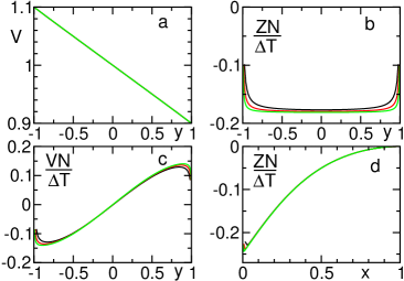
Numerical solution - The stationary solution of Eq. (7) can be efficiently computed by exploiting the sparsity of the corresponding linear problem, as well as the symmetries of the unknowns ${\bf u}$, ${\bf v}$ and ${\bf z}$. The elements of ${\bf C}$ can be thereby obtained from transformation (11). The diagonal elements of $\bf C$ correspond to the temperature profile. This is illustrated in Fig. 1a, where both $V_{ii}$ and $U_{ii}$ are plotted versus $y\equiv 2i/N-1$ for $k=2$ and different system sizes. The linear profile confirms the validity of Fourier’s law, as expected in the presence of an on-site potential rep . All the other $\bf C$ elements are of order $\mathcal{O}(1/N)$ and proportional to the temperature difference $\Delta T$ and are, therefore, scaled accordingly in the other panels of Fig. 1. The upper-diagonal of $\bf Z$ is plotted in panel (b); because of the antisymmetry of $\bf z$, $Z_{i-1,i}$ coincides with the deterministic component $J_{i}^{d}$ of the flux (see Eq. (9)). The singular behaviour at the extrema is a consequence of $J_{i}^{d}$ vanishing at the boundaries, where the particles are not free to move. The behavior of $\bf V$ along the upper diagonal is presented in Fig. 1c; it basically quantifies the $1/N$ finite-size deviations exhibited by the temperature profile. Finally, the dependence of $\bf Z$ along the principal antidiagonal [$x=(i-j)/N$] is shown in Fig. 1d, where one can notice a slow decay of the correlations. This is analogous to what found in purely stochastic models giardina ; young and is believed to be a generic feature of nonequilibrium stationary states jona .

Figure 1: (Color online) Some elements of the covariance matrix $\bf C$ (properly normalized) for $k=2$, $\omega=1$, $\gamma=1$, $\lambda=1$, $T_{+}=1.1$, $T_{-}=0.9$ and different chain sizes $N=128,256,512$; (a) $U_{i,i}=V_{i,i}=T_{i}$, (b) $NZ_{i,i+1}/\Delta T$, (c) $NV_{i,i+1}/\Delta T$, (d) $NZ_{i,N+1-i}$ (antidiagonal).

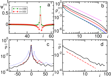
Principal component analysis - Once the covariance matrix is known, it is natural to determine its eigenvalues $\lambda^{(\nu)}$ ($\nu=1,\ldots,2N$) – that we assume to be ordered from the largest to the smallest one – and the corresponding normalized eigenvectors, that are denoted as $(\phi^{(\nu)}_{1},\ldots,\phi^{(\nu)}_{N},\psi^{(\nu)}_{1},\ldots,\psi^{(\nu)}_{N})$. Since $\bf C$ is almost diagonal, $\lambda^{(\nu)}$ yields the temperature profile and each of the two eigenvector components are localized. A less obvious fact is that the eigenvalues come in almost degenerate pairs (the relative difference being much smaller than $1/N$) and that the $\phi$ and $\psi$ components of corresponding eigenvectors are localized around the same site $m=\nu/2$ (see Fig. 2a, where the $\psi$ components are plotted for $\nu=100,101$). We interpret this by saying that any pair $(\nu,\nu+1)$ of eigenvectors identifies a single, localized, degree of freedom at equilibrium with a “temperature” $\lambda^{(\nu)}$ .

The eigenvector spatial structure can be fruitfully illustrated by plotting $\rho^{(\nu)}_{i}=[\phi_{i}^{(\nu)}]^{2}+[\psi_{i}^{(\nu)}]^{2}+[\phi_{i}^{(\nu+1)}]^{2}+[\psi_{i}^{(\nu+1)}]^{2}$. In Fig. 2b, we see that the vector width does not depend on the system size, which only determines the extension of the tails. Moreover, Fig. 2b shows also that the squared envelope decays as a power-law from its localization center, $\rho^{(\nu)}_{i}\approx[\ell/|i-m|]^{2}$ perturb . This defines a typical length $\ell$ that can be interpreted as the minimal size of the spatial region that is necessary to ensure a local thermal equilibrium, a sort of mean free path. This interpretation is supported by the fact that $\ell$ decreases upon increasing the strength $\gamma$ of the stochastic process, which is the only thermalization mechanism in the bulk.

Figure 2: (Color online) Localized structure of the eigenvectors of $\bf C$. The upper panels correspond to the model and parameter values of Fig. 1: (a) $\psi$ components of the vectors $\nu=100,101$ for $N=200$; (b) the squared envelope $\rho_{i}^{(\nu)}$ defined in the text for $N=400$ with $\gamma=2$ (dashed line) and $N=800$ with $\gamma=0.5,1,2$ (solid lines from top to bottom). (c) $\overline{\rho}=\sum_{\nu=\nu_{1}}^{\nu_{2}}\rho^{(\nu)}_{i}$: FPU model for $N=511$, $\nu_{1}=150$, $\nu_{2}=350$ (dotted line), unpinned case ($\gamma=0.4$) for $N=512$, $\nu_{1}=150$, $\nu_{2}=350$ (solid line) and $N=256$, $\nu_{1}=75$, $\nu_{2}=175$ (dashed line); (d) same data in log-log scale for the unpinned case ($N=512$). The straight lines have a slope $-2$ in (b) and $-1.5$ in (d).

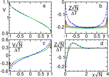
The unpinned case - The limit case of vanishing pinning force, $k=0$, is of particular interest. Indeed, here the total momentum is conserved and we expect an anomalous behaviour, i.e. a diverging finite-size thermal conductivity NR02 ; rep . As shown in Fig. 3a the temperature profile (solid line) is no more linear. Remarkably, we find also that all the nondiagonal elements are in this case of order $\mathcal{O}(1/\sqrt{N})$ (see the solid lines in Fig. 3b,c and d). In particular, through Eq. (9) this implies that the heat conductivity diverges as $\sqrt{N}$, in agreement with the linear response prediction BBO06 . This observation is supported by analytical arguments based on multiple-scale expansion of Eq. (7) in the smallness parameter $1/\sqrt{N}$ unp . A second remarkable difference with the case $k>0$ is the exponential decay of the off-diagonal terms, the decay length scaling as $\sqrt{N}$. For instance, in Fig. 3d (solid line) the elements along the antidiagonal of the matrix $\bf Z$ are plotted versus $x\sqrt{N}=(i-j)/\sqrt{N}$; similar curves are obtained for the same elements of the matrices $\bf U$ and $\bf V$.

On the other hand, the principal component analysis reveals that the eigenvalues still appear in almost degenerate pairs and the eigenvectors are localized (see Fig. 2c), although the tails decay with a slower power-law exponent, close to 1.5 (see Fig. 2d).

Figure 3: (Color on line) The same matrix elements as in Fig. 1 in the absence of an on-site potential $k=0$ and for $\gamma=0.4$. The three solid lines refer to $N=128$, 256, and 512. The dashed lines are obtained by simulation of a chain of 511 quartic FPU oscillators.

Comparison with a nonlinear model - In order to assess the generality of the scenario resulting from the stochastic model, it is crucial to investigate also a nonlinear deterministic model. We have considered the Fermi-Pasta-Ulam (FPU) chain with a purely quartic interparticle potential $(q_{i+1}-q_{i})^{4}/4$ LLP03 . We have implemented Eq. (Nonequilibrium Invariant Measure under Heat Flow), by working with stochastic heat baths in the limit of a small mass for the reservoir’s particles rep . This choice allows us to use a symplectic integrator and thereby to use “large” time steps ($10^{-2}$), still obtaining accurate results. The covariance matrix is then estimated by time averaging and is thus affected by the unavoidable statistical fluctuations (we have sampled about $5\times 10^{7}$ data points separated by one time unit). For a meaningful comparison, the $Q$ variables (11) are chosen to be $\Omega_{i}(q_{i+1}-q_{i})$, where $\Omega_{i}$ is a renormalized frequency that can be determined by imposing that the effective harmonic potential energy equals the kinetic energy. The homogeneity of the potential suggests setting $\Omega_{i}=\zeta T_{i}^{1/4}$; we have found that the best overlap between kinetic and potential energy is obtained for $\zeta=1.4$ AC03 . The results obtained for a chain of 511 oscillators are plotted in Fig. 3 (dashed lines), where the same $\sqrt{N}$ scaling of variables as in the unpinned stochastic model is implicitly assumed. Even though we should notice that $\gamma=0.4$ for the stochastic model has been selected to yield the best agreement with the temperature profile of the FPU model, the similarity between the deterministic and the stochastic model is quite striking and extends to the temperature deviations as well as to the behavior of the off-diagonal terms. The only elements that are significantly different are the upper diagonal terms of $\bf Z$ (see Fig. 3b). Statistical fluctuations prevent an accurate analysis of the single eigenvectors. In order to reduce their effects, we have decided to average a subset of eigenvectors around their localization center. The results presented in Fig. 2c (the average, denoted by $\bar{\rho}$, is performed over the eigenvectors from 150 to 350) reveal that also the eigenvectors of the FPU model are localized (the side peaks seem to be a finite-size effect, as they tend to disappear upon increasing the system size). A quantitative analysis of the decay rate is out of question.

The study of the above models has shown that the key features of nonequilibrium steady states are captured by principal component analysis and are contained in the statement that, the invariant measure can be effectively approximated as the product of independent Gaussians for the collective, localized mode amplitudes. The variances are the local temperatures.

In order to further explore the validity of this claim, we have studied the fluctuations of the single mode amplitudes and the correlations between pairs of such modes, going beyond the second cumulants. Within the numerical accuracy, we have not found any deviation from the assumption of a purely Gaussian distribution, even in the FPU model. We can also conjecture that the Gaussian assumption should become exact in the thermodynamic limit for model (Nonequilibrium Invariant Measure under Heat Flow) . We want to point out that, to our knowledge, this is the first case where an explicit nontrivial, even if approximate, representation of the nonequilibrium invariant measure is given for Hamiltonian models. As a further development, the stochastic model should be modified to reproduce quantitatively the universal scaling laws predicted for a generic system NR02 , as well as to analyse the corresponding modifications on the structure of the measure.

We acknowledge useful discussions with G. Basile and S. Olla. One of us (AP) wishes to thank the Erwin Schrödinger Institute for profitable exchanges of ideas.

References

- (1) For a recent overview see L. Bertini et al., J. Stat. Mech. P07014 (2007) and references therein: in particular, B. Derrida, J. L. Lebowitz and E. R. Speer, J. Stat. Phys. 107, 599 (2002), L. Bertini et al., J. Stat. Phys. 107, 635 (2002), J.R. Dorfman , T.R. Kirkpatrick and J.V. Sengers, Annu. Rev. Phys. Chem. 45, 213 (1994).
- (2) S. Lepri, R. Livi, A. Politi, Phys. Rep. 377, 1 (2003).
- (3) Z. Rieder, J.L. Lebowitz, E. Lieb, J. Math. Phys. 8 1073 (1967).
- (4) C. Kipnis, C. Marchioro, E. Presutti, J. Stat. Phys. 27 65 (1982).
- (5) C. Giardinà, J. Kurchan, and F. Redig, J. Math. Phys. 48, 033301 (2007).
- (6) C. Bernardin and S. Olla, J. Stat. Phys. 121, 271 (2005).
- (7) F. Bonetto, J.L. Lebowitz, L. Rey-Bellet, in: A. Fokas, A. Grigoryan, T. Kibble and B. Zegarlinski (Eds.), Mathematical Physics 2000, Imperial College, London, 2000.
- (8) I.T. Jolliffe, Principal Component Analysis, Springer Series in Statistics, Springer, New York, 2002.
- (9) G. Basile, C. Bernardin, and S. Olla, Phys. Rev. Lett. 96, 204303 (2006).
- (10) O. Narayan, S. Ramaswamy, Phys. Rev. Lett. 89, 200601 (2002).
- (11) K. K. Lin and L.S. Young, J. Stat. Phys. 128, 607 (2007).
- (12) By evaluating corrections to to the eigenvectors of in the limit, simple but lengthy calculations allow to justify this power law.
- (13) This value is close to the value obtained from the renormalization of phonon dispersion (at unit energy density) as computed in C. Alabiso, M. Casartelli, J. Phys. A: Math. Gen. 34 1223 (2001).
- (14) A. Politi (unpublished).
- (15) S. Lepri, R. Livi, A. Politi, Phys. Rev. E 68 067102 (2003).