An Infinite Family of Self-consistent Models for Axisymmetric Flat Galaxies

Abstract

We present the formulation of a new infinite family of self-consistent stellar models, designed to describe axisymmetric flat galaxies. The corresponding density-potential pair is obtained as a superposition of members belonging to the generalized Kalnajs family, by imposing the condition that the density can be expressed as a regular function of the gravitational potential, in order to derive analytically the corresponding equilibrium distribution functions (DF). The resulting models are characterized by a well-behaved surface density, as in the case of generalized Kalnajs discs. Then, we present a study of the kinematical behavior which reveals, in some particular cases, a very satisfactory behavior of the rotational curves (without the assumption of a dark matter halo). We also analyze the equatorial orbit’s stability and Poincaré surfaces of section are performed for the 3-dimensional orbits. Finally, we obtain the corresponding equilibrium DFs, using the approaches introduced by Kalnajs (1976) and Dejonghe (1986).

1 Introduction

The obtention of density-potential pairs (PDP) corresponding to idealized thin discs is a problem of great astrophysical relevance, motivated by the fact that the main part of the mass in many galaxies is concentrated in an stellar flat distribution, usually assumed as axisymmetric (Binney & Tremaine (1987)). Once the potential-density pair (PDP) is formulated as a model for a galaxy, usually the next step is to find the corresponding distribution function (DF). This is one of the fundamental quantities in galactic dynamics specifying the distribution of the stars in the phase-space of positions and velocities. Although the DF can generally not be measured directly, there are some observationally accesible quantities that are closed related to the DF: the projected density and the light-of-sight velocity, provided by photometric and kinematic observations, are examples of DF’s moments. Thus, the formulation of a PDP with its corresponding equilibrium DFs establish a self-consistent stellar model that can be corroborated by astronomical observations.

Now then, there is a variety potential-density pairs for such flat stellar models, e.g. Wyse & Mayall (1942); Kuzmin (1956); Schmith (1956); Toomre (1963, 1964); Brandt & Belton (1962); Kalnajs (1972); González & Reina (2006). In particular, Toomre (1963, 1964) formulated a generalized family of models whose first member is the one introduced by Kuzmin (1956). This family represents a set of discs of infinite extension, derived by solving the Laplace equation in cylindrical coordinates subject to appropriated boundary conditions on the discs and at infinity.

Analogously, González & Reina (2006) obtained a family of finite thin discs (generalized Kalnajs discs) whose first member corresponds precisely to the well-known model derived by Kalnajs (1972). Such family was derived by using the Hunter’s method (1963), which is based in the obtention of solutions of Laplace equation in terms of oblate spheroidal coordinates, by imposing some appropriate conditions on the surface density. So, by requiring that the surface density behaves as a monotonously decreasing function of the radius, with a maximum at the center of the disk and vanishing at the edge, detailed expressions for the gravitational potential and the rotational velocity were obtained as series of elementary functions. Also, some two-integral distribution functions for the first four members of this family were recently obtained by Pedraza, Ramos-Caro & González (2008). Now then, as the generalized Kalnajs models correspond to discs of finite extension, they can be considered as more realistic descriptions of flat galaxies than the Toomre’s family.

In the present paper we formulate a new infinite set of finite thin discs, obtained by superposing the members of the generalized Kalnajs family in such a way that the resulting density surface can be expressed as a well behaved function of the gravitational potential. As it was pointed out by some authors, this is a fundamental requirement for the searching of equilibrium distribution functions (DF) describing such axisymmetric systems (see for example, Fricke (1962), Hunter & Quian (1993), Jiang & Ossipkov (2007)). Thus, the new family formulated here has the advantage of easily providing the corresponding two-integral DFs.

Furthermore, the models have two additional advantages. In one hand, the mass surface density is well-behaved, as in the case of generalized Kalnajs discs, having a maximum at the center and vanishing at the edge. Moreover, the mass distribution of the higher members of the family is more concentrated at the center. On the other hand, the rotation curves are better behaved than in the Kalnajs discs. We found that, in some cases, the circular velocity increases from a value of zero at the center of the disc, then reaches a maximum at some critical radius and, after that, remains approximately constant. As it is known, such behavior has been observed in many disclike galaxies.

Now, apart from the circular velocity, there are two important quantities concerning to the interior kinematics of the models: the epicyclic and vertical frequencies, which describe the stability against radial and vertical perturbations of particles in quasi-circular orbits. We found that the models formulated here are radially stable whereas vertically unstable, which is a characteristic inherited from the generalized Kalnajs family (Ramos-Caro, López-Suspez & González (2008)). When we deal with three dimensional orbits, there are also a common feature between the new models and the Kalnajs family: the phase space structure of disc-crossing orbits, that can be viewed through the Poincaré surfaces of section, is composed by shape-of-ring KAM curves and prominent chaotic zones. However, there are certain situations in which the chaoticity disappears and the 3-dimensional motion of test particles is completely regular. In such cases, one can suggest the existence of a third integral of motion, as in the case of Stäckel and Kuzmin potentials.

Finally, in order to formulate the new family as a set of self-consistent stellar models, we shall deal with the problem of obtaining the corresponding equilibrium DFs. By Jeans’s theorem, they are functions of the isolating integrals of motion that are conserved in each orbit. Some authors have shown that, if the density can be written as a function of the gravitational potential, it is possible to find such kind of two-integral DFs (see Eddington (1916); Fricke (1952); Kalnajs (1976); Jiang and Ossipkov (2007)). In this paper we shall adopt the approach introduced by Kalnajs (1976), which fits quite well to axisymmetric disc-like systems. Then, starting from the DFs derived from this method, a second kind of DFs is obtained by using the formulae introduced by Dejonghe (1986), that takes into account the principle of maximum entropy. These DFs describe stellar systems with a preferred rotational state.

Accordingly, the paper is organized as follows. First, at section 2, we obtain the potential-density pairs for the new family of thin disc models. Then, at section 3, we study the motion of test particles around these new galactic models and, at section 4, we derive the distribution functions associated with the models. Finally, at section 5, we summarize our main results.

2 A New Family of Thin Disc Models

2.1 The generalized Kalnajs discs

In this subsection we summarize the principal features of the generalized Kalnajs family, introduced by González & Reina (2006), an infinite family of axially symmetric finite thin discs. The mass surface density of each disc (labeled with the positive integer $n$) is given by

$$\Sigma_{n}(R)=\Sigma_{c}^{(n)}\left[1-\frac{R^{2}}{a^{2}}\right]^{n-1/2},$$ (1)

where $M$ is the total mass, $a$ is the disc radius and $\Sigma_{c}^{(n)}$ are constants given by

$$\Sigma_{c}^{(n)}=\frac{(2n+1)M}{2\pi a^{2}}.$$ (2)

Such mass distribution generates an axially symmetric gravitational potential, that can be written as

$$\Phi_{n}(\xi,\eta)=-\sum_{j=0}^{m}C_{2j}q_{2j}(\xi)P_{2j}(\eta).$$ (3)

Here, $P_{2j}(\eta)$ and $q_{2j}(\xi)=i^{2j+1}Q_{2j}(i\xi)$ are the usual Legendre polynomials and the Legendre functions of the second kind respectively, $-1\leq\eta\leq 1$ and $0\leq\xi<\infty$ are spheroidal oblate coordinates, related to the usual cylindrical coordinates $(R,z)$ through the relations

$$R^{2}=a^{2}(1+\xi^{2})(1-\eta^{2}),\qquad z=a\eta\xi,$$ (4)

in such a way that the discs are located at $\xi=0$ and $\eta=\sqrt{1-R^{2}/a^{2}}$. Finally, the $C_{2j}$ are constants given by

$$C_{2j}=\frac{MG\pi^{1/2}(4j+1)(2n+1)!}{a2^{2n+1}(2j+1)(n-j)!\Gamma(n+j+\frac{3}{2})q_{2j+1}(0)},$$

where $G$ is the gravitational constant.

As it was shown by González & Reina (2006), in these models the surface density is a monotonously decreasing function of the radius, with a maximum at the center of the disk and vanishing at the edge, being the mass distribution of the higher members of the family more concentrated at the center. On the other hand, the corresponding rotation curves behave as follows: for $n=1$, the circular velocity is proportional to the radius, whereas for the other members of the family it increases from a value of zero at the center of the discs, then reaches a maximum at a critical radius and, finally, decreases to a finite value at the edge. Besides, the critical radius decreases as the value of $n$ increases.

2.2 Formulation of the New Family

Now, we will show that it is possible to formulate a new family of stellar models by performing a linear combination of generalized Kalnajs discs, in such a way that the new surface densities can be written as polynomials of the new potentials. As it was quoted, this is a basic requirement for the derivation of equilibrium DFs through the Kalnajs formalism sketched above. In particular, we are interested on to derive a simple relation between the relative potential on the disc and the surface density.

At first, note that $\Phi_{n}(0,\eta)$, given by (3), can be rewritten as

$$\Phi_{n}(0,\eta)=-\sum_{s=0}^{n}\sum_{r=0}^{s}A_{sr}\eta^{2s-2r},$$ (5)

where $A_{sr}$ are constants defined as

$$A_{sr}=\frac{(-1)^{r}(4s-2r)!C_{2s}q_{2s}(0)}{2^{2s}r!(2s-2r)!(2s-r)!},$$ (6)

and the relation (5) was derived by introducing the identity (Arfken (2005))

$$P_{2s}(\eta)=\sum_{r=0}^{s}\frac{(-1)^{r}(4s-2r)!}{2^{2s}r!(2s-2r)!(2s-r)!}\eta^{2s-2r}.$$ (7)

From (5) we note that the maximum value of the gravitational potential on the $n$th disc is $\Phi_{n}(0,0)$. Therefore, we define the relative potential on such a disc as

$$\Psi_{n}(\eta)=\Phi_{n}(0,0)-\Phi_{n}(0,\eta).$$ (8)

Now, suppose that we can choose a linear combination of those $\Psi_{n}$ leading to a new relative potential $\tilde{\Psi}_{m}$ of the form

$$\tilde{\Psi}_{m}=\sum_{n=1}^{m}B_{n}\Psi_{n}=A_{m0}\eta^{2m},$$ (9)

where $B_{n}$ are constants that can be determined from $A_{nr}$ and $C_{n}$ (see section 2.3).

The new relative potential $\tilde{\Psi}_{m}$ is generated by a new mass distribution described by a surface density $\tilde{\Sigma}_{m}$ that is also a linear combination of generalized Kalnajs discs $\Sigma_{m}$. That is

$$\tilde{\Sigma}_{m}(R)=\sum_{n=1}^{m}B_{n}\Sigma_{c}^{(n)}\eta^{2n-1}.$$ (10)

From this relation and (9), we can note that $\tilde{\Sigma}_{m}$ can be rewritten as

$$\tilde{\Sigma}_{m}(R)=\sum_{n=1}^{m}B_{n}\Sigma_{c}^{(n)}\left(\frac{\tilde{\Psi}_{m}}{A_{m0}}\right)^{(2n-1)/(2m)}.$$ (11)

Thus, we can see that this new family of discs is characterized by the fact that the surface density can be split as a combination of powers of the relative potential. This important fact makes viable the further derivation of two integral DFs for the whole family (see section 4), that can be considered as a set of self-consistent galactic models. Now, the above statements are only true if we can determinate the constants $B_{n}$, introduced in (9). In the next subsection, we show a procedure that, by using the orthogonality properties of $P_{n}$, leads to a recurrence relation expressing $B_{n}$ in terms of $A_{nr}$ and $C_{n}$.

2.3 Calculation of $B_{n}$

According to definitions (8) and (3), the relative potential associated to the generalized Kalnajs discs can be written as

$$\Psi_{m}(\eta)=\sum_{n=0}^{m}\tilde{C}_{n}P_{2n}(\eta),$$ (12)

where $\tilde{C}_{n}$ are constants defined by

$$\tilde{C}_{n}=C_{2n}q_{2n}(0)-\delta_{0n}\sum_{i=0}^{m}C_{2i}q_{2i}(0)P_{2i}(0).$$ (13)

So, by introducing (12) into (9), $\tilde{\Psi}_{m}$ can also be written in terms of Legendre polynomials as

$$\tilde{\Psi}_{m}=\sum_{n=0}^{m}\sum_{i=0}^{n}B_{n}\tilde{C}_{i}P_{2i}(\eta)=\sum_{n=0}^{m}D_{n}P_{2n}(\eta),$$ (14)

where $D_{n}$ are constants to be determined. Here, it is important to note that these $D_{n}$ are such that

$$D_{m}\,\;\;\, =B_{m}\tilde{C}_{m},$$ (15a)

$$D_{m-1} =B_{m}\tilde{C}_{m-1}+B_{m-1}\tilde{C}_{m-1},$$ (15b)

$$D_{m-2} =B_{m}\tilde{C}_{m-2}+B_{m-1}\tilde{C}_{m-2}+B_{m-2}\tilde{C}_{m-2},$$ (15c)

$$\;\;\vdots$$

$$D_{m-k} =\tilde{C}_{m-k}\sum_{i=0}^{k}B_{m-i}.$$ (15d)

The above equations can be written in a compact way as

$$D_{n}=\tilde{C}_{n}\sum_{i=0}^{m-n}B_{m-i},$$ (16)

which summarizes the previous series of recurrence relations.

Now, let us come to the problem of calculating $D_{n}$. According to (9) and (14), we have

$$\sum_{n=0}^{m}D_{n}P_{2n}(\eta)=A_{m0}\eta^{2m},$$ (17)

and by using the orthogonality properties of Legendre polynomials, we obtain

$$D_{n}=A_{m0}\frac{4n+1}{2}\int_{-1}^{1}\eta^{2m}P_{2n}(\eta)d\eta,$$

that reduces to

$$D_{n}=A_{m0}\left[\frac{\pi^{1/2}(4n+1)\Gamma(2m+1)}{2^{2m+1}\Gamma(1+m-n)\Gamma(m+n+\begin{matrix}\frac{3}{2}\end{matrix})}\right],$$ (18)

in such a way that, by using (16), we can determine the constants $B_{n}$. In order to do this, note that equations (15a)-(15d) give us recurrence relations: from (15a) we obtain $B_{m}$, from (15b) we obtain $B_{m-1}$, and so on. In general, we have

$$B_{m}\,\;\;\, =\frac{D_{m}}{\tilde{C}_{m}}=1,$$ (19a)

$$B_{m-1} =\frac{D_{m-1}}{\tilde{C}_{m-1}}-B_{m},$$ (19b)

$$B_{m-2} =\frac{D_{m-2}}{\tilde{C}_{m-2}}-B_{m}-B_{m-1},$$ (19c)

$$\;\;\vdots$$

$$B_{m-k} =\frac{D_{m-k}}{\tilde{C}_{m-k}}-\sum_{i=0}^{k-1}B_{m-i},\quad\mathrm{for}\quad k\geq 1,$$ (19d)

relations that can be summarized as

$$B_{n}=\frac{D_{n}}{\tilde{C}_{n}}-\sum_{i=0}^{m-n-1}B_{m-i},\quad\mathrm{for}\quad n\leq m-1.$$ (20)

Figure 1: We plot the mass surface density $\tilde{\Sigma}_{2}$, $\tilde{\Sigma}_{3}$, $\tilde{\Sigma}_{4}$ and $\tilde{\Sigma}_{5}$ (from bottom to top in the left edge), given by (22), where the parameters $B_{n}$ are determined by (20). Since the resulting densities are negative in some ranges, we must to correct $B_{1}$.

In table 1 we show the values of $B_{n}$ for the first four models, i.e. $m=2,3,4,5$. Although we have solved the problem of finding these constants, there is another inconvenient. If one introduces such coefficients in (10), the corresponding surface density is negative for certain ranges of $R$, as it is shown in figure 1, where we plot the resulting $\tilde{\Sigma}$ for the first four models. However, this problem can be solved by correcting $B_{1}$, i.e. the coefficient corresponding to the dominant term in (10). In the next subsection, we show that it is possible to define minimum values for $B_{1}$, corresponding to each model, in such a way that all of they be described by positive surface densities.

m	$B_{1}$	$B_{2}$	$B_{3}$	$B_{4}$	$B_{5}$
2	$-5/8$	$1$
3	$-35/192$	$-7/12$	$1$
4	$-105/1024$	$-21/128$	$-9/16$	$1$
5	$-1155/16384$	$-231/2560$	$-99/640$	$-11/20$	$1$

Table 1: Constants $B_{n}$ for the first four models: $m=2,3,4,5$

2.4 Correction of $B_{1}$

From here on, we consider $B_{1}$ as an arbitrary parameter that can be chosen in such a way that $\tilde{\Sigma}\geq 0$, in the range $0\leq R\leq a$. For each model, we expect that $B_{1}$ has a lower limit but does not has an upper limit. The reason is that, according to (1), we have

$$\lim_{R\rightarrow a}\frac{\mathrm{d}\Sigma_{m}}{\mathrm{d}R}=\left\{\begin{tabular}[]{cc}$-\infty$&for $m=1$,\\ $0$&for $m\geq 2$.\\ \end{tabular}\right.$$ (21)

This means that the behavior of $\Sigma_{1}$, for $R\rightarrow a$, differs from the remaining density surfaces, characterized by a rate of change tending asymptotically to $0$ at the disc edge. Thus, it is evident that one always can find a minimum value $B_{1\mathrm{min}}$, such that the product $B_{1\mathrm{min}}\Sigma_{1}$ is larger than any linear combination of $\Sigma_{2},\Sigma_{3},\ldots$.

In the particular case corresponding to the new models here formulated, the surface density can be split as

$$\tilde{\Sigma}_{m}(R,B_{1}) = B_{1}\Sigma_{c}^{(1)}\left(1-\frac{R^{2}}{a^{2}}\right)^{1/2}$$ (22)

$$+\sum_{n=2}^{m}B_{n}\Sigma_{c}^{(n)}\left(1-\frac{R^{2}}{a^{2}}\right)^{n-1/2},$$

where the coefficients $B_{n}$, for $n\geq 2$, are given by (20). A simple way to find $B_{1\mathrm{min}}$, is by demanding that $\tilde{\Sigma}_{m}$ has a minimum (equal to $0$) at $B_{1}=B_{1\mathrm{min}}$ and $R=R_{\mathrm{min}}$. That is, we demand that the following two equations holds:

$$\left.\frac{\mathrm{d}\tilde{\Sigma}(R,B_{1\mathrm{min}})}{\mathrm{d}R}\right|_{R=R_{\mathrm{min}}}=0,$$ (23)

$$\tilde{\Sigma}(R_{\mathrm{min}},B_{1\mathrm{min}})=0.$$ (24)

The relation (23) imposes the condition that the surface density has a minimum at $B_{1}=B_{1\mathrm{min}}$ and $R=R_{\mathrm{min}}$, while through the relation (24) we demand that its value at such critical point is $0$.

Figure 2: We plot the mass surface density (a) $\tilde{\Sigma}_{2}$, (b) $\tilde{\Sigma}_{3}$, (c) $\tilde{\Sigma}_{4}$, (d) $\tilde{\Sigma}_{5}$, for different values of the parameter $B_{1}$. In each case we start with $B_{1}=B_{1min}$ (lower curve), given by table 2. The remaining curves, from bottom to top, corresponds to increments of $0.01$ in $B_{1}$, starting from $B_{1min}$.

We find numerically the lower bounds of $B_{1}$ for the first four members of the new family and they are showed in table 2. The corresponding surface densities, for different values of $B_{1}>B_{1\mathrm{min}}$, are plotted in figure 2. We note that, in all of these cases, the mass concentration start in $0$ for $R=a$ and increases towards the disc bulge. Moreover, such concentration increases with $m$.

m	$B_{1min}$	$B_{2}$	$B_{3}$	$B_{4}$	$B_{5}$
2	$0$	$1$
3	$0.101273$	$-7/12$	$1$
4	$0.128914$	$-21/128$	$-9/16$	$1$
5	$0.143207$	$-231/2560$	$-99/640$	$-11/20$	$1$

Table 2: Corrected constants $B_{n}$ for the first four models: $m=2,3,4,5$

Finally, the gravitational potential corresponding to the new family, derived as a linear combination of generalized Kalnajs discs, can be cast as

$$\tilde{\Phi}_{m}(\xi,\eta)=-\sum_{n=1}^{m}\sum_{k=0}^{n}B_{n}C_{2k}q_{2k}(\xi)P_{2k}(\eta),$$ (25)

where $B_{n}$ are given by (20), for $n\geq 2$ and $B_{1}$ is an arbitrary parameter with lower bound determined by (23)-(24).

3 Kinematics of the New Family

In this section we study the motion of test particles around the galactic models formulated above. Since each $\tilde{\Phi}_{m}$ is static and axially symmetric, the specific energy $E$ and the specific axial angular momentum $\ell$ are conserved along the particle motion. This fact restricts such motion to a three dimensional subspace of the $(R,z,V_{R},V_{z})$ phase space. By defining an effective potential $\Phi_{m}^{*}$ as

$$\Phi_{m}^{*}=\tilde{\Phi}_{m}+\frac{\ell^{2}}{2R^{2}},$$ (26)

the motion will be determined by the equations (Binney & Tremaine (1987))

$$\dot{R} ={V}_{R},$$ (27a)

$$\dot{z} ={V}_{z},$$ (27b)

$$\dot{V}_{R} =-\frac{\partial\Phi_{m}^{*}}{\partial R},$$ (27c)

$$\dot{V}_{z} =-\frac{\partial\Phi_{m}^{*}}{\partial z},$$ (27d)

together with

$$E=\frac{1}{2}({V}_{R}^{2}+{V}_{z}^{2})+\Phi_{m}^{*},$$ (28)

which gives the total energy of the particle.

Relations (27a)-(28) are the basic equations that determine the motion of a particle with specific axial angular momentum $\ell$ and energy $E$, in cylindrical coordinates. At first, we restrict our attention on particles belonging the disc, i.e. the interior kinematics, in order to describe rotation curves (for circular orbits) and the stability of nearly circular orbits (by deriving the epicyclic and vertical frequencies). Then, we shall focus on three dimensional motion, in particular, the case of disc crossing orbits. In such case, we use $z=0$ surfaces of section, in order to illustrate the regularity or chaoticity characterizing those orbits.

3.1 Interior Kinematics

Figure 3: We plot the rotation curves for (a) $m=2$, (b) $m=3$, (c) $m=4$, (d) $m=5$, for the same values of parameter $B_{1}$ as in figure 2. The lower curves corresponds to $B_{1min}$ and the upper curves corresponds to larger values of $B_{1}$.

We start by pointing out that the system (27a) has equilibrium points at $V_{R}=V_{z}=z=0$, $R=R_{c}$, where $R_{c}$ must satisfy the equation

$$\left(\frac{\partial\Phi_{m}^{*}}{\partial R}\right)_{(R_{c},0)}=-\frac{\ell^{2}}{R_{c}^{3}}+\left(\frac{\partial\tilde{\Phi}_{m}}{\partial R}\right)_{(R_{c},0)}=0,$$ (29)

that is the condition for a circular orbit in the plane $z=0$. In other words, the equilibrium points of (27a) occur when the test particle describes equatorial circular orbits of radius $R_{c}$, specific axial angular momentum given by

$$\ell_{c}=\pm\sqrt{R_{c}^{3}\left(\frac{\partial\tilde{\Phi}_{m}}{\partial R}\right)_{(R_{c},0)}}\>\>,$$ (30)

and specific energy

$$E=\Phi_{m}^{*}(R_{c},0).$$ (31)

The subscript $c$ in $\ell_{c}$ indicates that we are dealing with circular orbits.

Figure 4: Quadratic epicyclic frequency as a function of $R$ for the cases (a) $m=2$, (b) $m=3$, (c) $m=4$, (d) $m=5$. We use the same values of parameter $B_{1}$ as in figure 2. The lower curves corresponds to $B_{1min}$ and the upper curves corresponds to larger values of $B_{1}$. In all of these cases, we note a prominent range of radial stability. Such range increases with $B_{1}$.

Figure 5: Quadratic vertical frequency as a function of $R$ for the cases (a) $m=2$, (b) $m=3$, (c) $m=4$, (d) $m=5$. We use the same values of parameter $B_{1}$ as in figure 2. The lower curves corresponds to $B_{1min}$ and the upper curves corresponds to larger values of $B_{1}$. The range of vertical stability is small and increases with $B_{1}$.

Now, a feature of special interest is the circular velocity $V_{c}=\ell_{c}R_{c}$ (sometimes denoted by $V_{\varphi}$), which can be directly compared with astronomical observations. Then, it is convenient to express $V_{c}$ as a function of the radius. From (30), we can write the magnitude of the circular velocity as $V_{c}^{2}=R\left(\partial\tilde{\Phi}_{m}/\partial R\right)_{z=0}$. In figure 3, we plot $V_{c}(R)$ corresponding to the first four models of the new family of discs. For $B_{1}=B_{1\mathrm{min}}$ the rotation curves has a maximum and then decreases to a constant value, in a similar fashion that the behavior of generalized Kalnajs discs (González & Reina (2006)). Moreover, the maximum of the rotation curve is at an even smaller radius when the value of m increases. Now, in the case in which $B_{1}$ is very large, the curve approximates to a straight line, as a consequence of the dominance of term associated with the usual Kalnajs disc. On the other hand, for intermediate values of $B_{1}$ we note an interesting feature: when the rotation curve reaches its maximum, it remains nearly constant, as it is the case in many real galaxies.

In order to study the stability of these trajectories under small radial and vertical ($z$-direction) perturbations, we analyze the nature of quasi-circular orbits. They are characterized by an epicycle frequency $\kappa$ and a vertical frequency $\nu$, given by (Binney & Tremaine 1987)

$$\kappa^{2}=\left(\frac{\partial^{2}\Phi_{m}^{*}}{\partial R^{2}}\right)_{(R_{c},0)},\>\>\>\>\>\>\>\>\>\>\nu^{2}=\left(\frac{\partial^{2}\Phi_{m}^{*}}{\partial z^{2}}\right)_{(R_{c},0)}.$$ (32)

This means that by introducing (30) in the second derivatives of $\Phi_{m}^{*}$ we obtain $\kappa^{2}$ and $\nu^{2}$ as functions of the radius. Values of $R$ such that $\kappa^{2}>0$ and (or) $\nu^{2}>0$ corresponds to stable circular orbits under small radial and (or) vertical perturbations, respectively. In figures 4 and 5 we show the behavior of the epicycle and vertical frequency, respectively, for the first four models and using the same values of $B_{1}$ as in figure 2. We note that these models are characterized by a prominent range of stability under radial perturbations. In particular, for $B_{1}>B_{1min}$, there will be radially stable orbits with radius in the range $0\leq R\leq a$. In contrast, there are prominent ranges of vertical instability. Such ranges tend to decreases when $m$ and $B_{1}$ increases. Thus, we can say that the stability under vertical perturbations, in quasi-circular orbits, improves in models with a large $m$.

3.2 Exterior Kinematics: Disc-crossing Orbits

In this section, we study the behavior of 3-dimensional motion, i.e. orbits outside the equatorial plane (except when they cross the plane $z=0$). As it was mentioned above, the motion is determined by (27a) and can be described in an effective phase space with three dimensions (there are two integrals of motion: $E$ and $\ell$). An adequate tool to investigate such orbits is the Poincaré surface of section, in order to find the chaotic and (or) regular regions characterizing the structure of the phase space.

In particular, we present numerical solutions of (27a)- (27d) for the case of bounded disc-crossing orbits. There are certain values of $E$ and $\ell$ for which they are confined to regions that contain the disc and will cross back and forth through it. As it was showed by Hunter (1993), this fact usually gives rise to many chaotic orbits due to the discontinuity in the $z$-component of the gravitational field, producing a fairly abrupt change in their curvatures. There is an important exceptional case of this behavior: the Kuzmin’s disc, characterized by an integrable potential of the form $\Phi=-GM[R^{2}+(a+|z|)^{2}]^{-1/2}$, with $a>0$. However, the so-called Kuzmin-like potentials, characterized by $\Phi(\varepsilon)$ where $\varepsilon=[R^{2}+(a+|z|)^{2}]^{1/2}$, are non-integrable and present the behavior mentioned above. The family of models formulated here present a very similar structure and we can expect an analogous dynamics. Each potential $\tilde{\Phi}_{m}(\xi,\eta)$ can be cast in a Kuzmin-like form if we take into account that, according to (4), $\xi=(R_{+}+R_{-})/2a$ and $\eta=(R_{+}-R_{-})/2ia$, where $R_{+}=[R^{2}+(z+ia)^{2}]^{1/2}$ and $R_{-}=[R^{2}+(z-ia)^{2}]^{1/2}$. Moreover, they are characterized by a z-derivative discontinuity in the disc, given by

$$\left(\frac{\partial\tilde{\Phi}_{m}}{\partial z}\right)_{z=0^{+}}=-\left(\frac{\partial\tilde{\Phi}_{m}}{\partial z}\right)_{z=0^{-}}=2\pi G\>\>\tilde{\Sigma}_{m}(R).$$ (33)

Despite the above relation makes the KAM theorem inapplicable, we also found a large variety of regular disc-crossing orbits.

In Figure 6, we show the $z=0$-surface of section corresponding to some orbits with $E=-1.245$ and $\ell=0.2$ (these same values are used to perform the next three surfaces of section), corresponding to a test particle moving around the model $m=2$ with $B_{1}=0.1$. As it was expected, from our experience with the generalized Kalnajs discs (Ramos-Caro, López-Suspez & González (2008)), this plot exhibits a variety of regular and chaotic trajectories. There is a regular central region conformed by two kinds of KAM curves: the central rings made by box orbits; a set of resonant islands chain (made by loop orbits) enclosing the rings. Moreover, there are two lateral regular zones of loop orbits that, as well as the central region, are enclosed by a sea of chaos. In figure 7, we show the effect of increasing $B_{1}$ in model $m=2$. Then, for the same initial conditions with $E=-1.245$ and $\ell=0.2$, the surface of section reveals an increasing in the chaotic region along with a distortion of the KAM curves in regular zones (for example, now the central torus are made only by box orbits).

One could expect similar chaotic surfaces of section for models $m=3,\ldots$, but what really happens is that for certain values of $B_{1}$ all the orbits are regular. This is the case illustrated in figure 8, where the Poincaré section, corresponding to a particle moving around the model $m=3$, reveals completely regular motion. This is a surprising fact, since in this kind of potentials chaos is the rule. If one increases $B_{1}$ (for example, from 0.2 to 1), as in the case of figure 9, we find again a prominent chaotic region enclosing some regular regions of KAM curves. Thus, the free parameter $B_{1}$, apart from determining some relevant features in equatorial orbits, plays an essential role in 3-dimensional motion and we can conjecture that, for certain values, it is possible to have a third integral of motion.

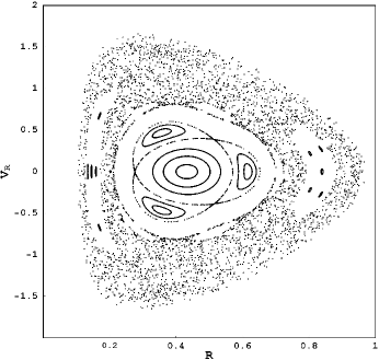
Figure 6: Surface of section for some orbits with $\ell=0.2$, $E=-1.245$, around the model $m=2$ with $B_{1}=0.1$.

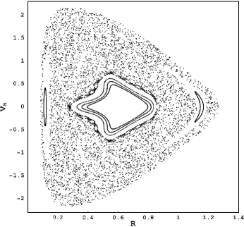
Figure 7: Surface of section for some orbits with $\ell=0.2$, $E=-1.245$, around the model $m=2$ with $B_{1}=0.5$.

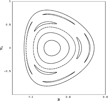
Figure 8: Surface of section for some orbits with $\ell=0.2$, $E=-1.245$, around the model $m=3$ with $B_{1}=0.2$. In this case we have only regular orbits

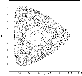
Figure 9: Surface of section for some orbits with $\ell=0.2$, $E=-1.245$, around the model $m=3$ with $B_{1}=1$. Now, a prominent chaotic region appears as a consequence of the overlapping of the lateral island chains, showed in the previous figure.

4 Two-Integral Distribution Functions

The derivation of the DFs, associated to the models constructed above, is particularly simple if we work in an adequate rotating frame, as it was pointed out by Kalnajs (1976). To begin with, we had seen that for a $B_{1}$ given by the recurrence relation (20) (from here on we denote it as $B_{1}^{*}$) the relative potential would be

$$\tilde{\Psi}_{m}^{*}=B_{1}^{*}\Psi_{1}+\sum_{n=2}^{m}B_{n}\Psi_{n}=A_{m0}\eta^{2m}.$$ (34)

On the other hand, if we choose a different $B_{1}$, the relative potential becomes

$$\begin{split}\tilde{\Psi}_{m}&=B_{1}\Psi_{1}+\sum_{n=2}^{m}B_{n}\Psi_{n}=A_{m0}\eta^{2m}+(B_{1}-B_{1}^{*})\Psi_{1},\\ &=A_{m0}\eta^{2m}+\begin{matrix}\frac{1}{2}\end{matrix}(B_{1}-B_{1}^{*})\Omega_{0}^{2}a^{2}\eta^{2},\end{split}$$ (35)

where $\Omega_{0}=[3\pi GM/(4a^{3})]^{1/2}$.

Now, let’s work in a a rotating frame with angular velocity $\Omega$. In this frame, the effective potential is defined as (Binney & Tremaine (1987))

$$\Phi_{e}=\Phi-\begin{matrix}\frac{1}{2}\end{matrix}\Omega^{2}R^{2}=\Phi+\begin{matrix}\frac{1}{2}\end{matrix}\Omega^{2}a^{2}(\eta^{2}-1),$$ (36)

and by choosing properly the constants, the relative-effective potential will be

$$\tilde{\Psi}_{e,m}=A_{m0}\eta^{2m}+\begin{matrix}\frac{1}{2}\end{matrix}(B_{1}-B_{1}^{*})\Omega_{0}^{2}a^{2}\eta^{2}-\begin{matrix}\frac{1}{2}\end{matrix}\Omega^{2}a^{2}\eta^{2}.$$ (37)

Note that if one chooses $\Omega$ as

$$\Omega=\pm\Omega_{0}\sqrt{B_{1}-B_{1}^{*}},$$ (38)

the term with $\eta^{2}$ vanishes and equation (37) reduces to

$$\tilde{\Psi}_{e,m}=A_{m0}\eta^{2m}.$$ (39)

Therefore, the relation between the density and the relative-effective potential can be written as

$$\tilde{\Sigma}_{m}(R)=\sum_{n=1}^{m}B_{n}\Sigma_{c}^{(n)}\left(\frac{\tilde{\Psi}_{e,m}}{A_{m0}}\right)^{(2n-1)/(2m)}.$$ (40)

Finally, by using the Kalnajs method (Kalnajs (1976)), we obtain that the DF corresponding to the $m$-model is given by

$$f_{m}(\varepsilon,L_{z})=\frac{1}{4\pi m}\sum_{n=1}^{m}\frac{B_{n}\Sigma_{c}^{(n)}(2n-1)A_{m0}^{-(2n-1)/(2m)}}{\left(\varepsilon+\Omega L_{z}-\begin{matrix}\frac{1}{2}\end{matrix}\Omega^{2}a^{2}\right)^{1-(2n-1)/(2m)}}.$$ (41)

The explicit DFs for the first 4 models and the associated $\Omega$, given by (38), are

$$f_{2} =\frac{3\Sigma_{c}^{(2)}A_{20}^{-3/4}}{4J^{1/4}}+\frac{B_{1}\Sigma_{c}^{(1)}A_{20}^{-1/4}}{4J^{3/4}},$$ (42a)

$$f_{3} =\frac{5\Sigma_{c}^{(3)}A_{30}^{-5/6}}{6J^{1/6}}-\frac{7\Sigma_{c}^{(2)}A_{30}^{-3/6}}{24J^{3/6}}+\frac{B_{1}\Sigma_{c}^{(1)}A_{30}^{-1/6}}{6J^{5/6}},$$ (42b)

$$f_{4} =\frac{7\Sigma_{c}^{(4)}A_{40}^{-7/8}}{8J^{1/8}}-\frac{45\Sigma_{c}^{(3)}A_{40}^{-5/8}}{128J^{3/8}}$$

$$-\frac{63\Sigma_{c}^{(2)}A_{40}^{-3/8}}{1024J^{5/8}}+\frac{B_{1}\Sigma_{c}^{(1)}A_{40}^{-1/8}}{8J^{7/8}},$$ (42c)

$$f_{5} =\frac{9\Sigma_{c}^{(5)}A_{50}^{-9/10}}{10J^{1/10}}-\frac{77\Sigma_{c}^{(4)}A_{50}^{-7/10}}{200J^{3/10}}$$

$$-\frac{99\Sigma_{c}^{(3)}A_{50}^{-5/10}}{1280J^{5/10}}-\frac{693\Sigma_{c}^{(2)}A_{50}^{-3/10}}{25600J^{7/10}}+\frac{B_{1}\Sigma_{c}^{(1)}A_{50}^{-1/10}}{10J^{9/10}},$$ (42d)

where $J=\varepsilon+\Omega L_{z}-\begin{matrix}\frac{1}{2}\end{matrix}\Omega^{2}a^{2}$ is the Jacobi’s integral and

$$A_{20} =\frac{45GM\pi}{128a}, \Omega_{2}^{2} =\frac{3\pi GM(5+8B_{1})}{32a^{3}},$$ (43a)

$$A_{30} =\frac{175GM\pi}{512a}, \Omega_{3}^{2} =\frac{3\pi GM(35+192B_{1})}{768a^{3}},$$ (43b)

$$A_{40} =\frac{11025GM\pi}{32768a}, \Omega_{4}^{2} =\frac{3\pi GM(105+1024B_{1})}{4096a^{3}},$$ (43c)

$$A_{50} =\frac{43659GM\pi}{131072a}, \Omega_{5}^{2} =\frac{3\pi GM(1155+16384B_{1})}{65536a^{3}}.$$ (43d)

Figure 10: We plot the DFs as functions of the Jacobi’s integral for (a) $m=2$, (b) $m=3$, (c) $m=4$, (d) $m=5$, for different values of the parameter $B_{1}$. The lower curves corresponds to $B^{\prime}_{1min}$ and the upper curves corresponds to larger values of $B_{1}$

It is easy to see that the DFs obtained by equation (41), for the cases $m\geq 3$, could be negative in some regions of the phase space corresponding to the physical domain. To avoid this inconvenient, it is necessary to impose a stronger condition for the constants $B_{1}$, in order to obtain well-defined distribution functions. To do this, we formulate the following equations (in a similar fashion as in subsection 2.4):

$$\left.\frac{\mathrm{d}f_{m}(J,B_{1\mathrm{min}}^{\prime})}{\mathrm{d}R}\right|_{J=J_{\mathrm{min}}}=0,$$ (44)

$$f_{m}(J_{\mathrm{min}},B_{1\mathrm{min}}^{\prime})=0.$$ (45)

Relation (44) imposes the condition that the DF has a minimum at $B_{1}=B^{\prime}_{1\mathrm{min}}$ and $R=R_{\mathrm{min}}$, while through the relation (45), we demand that its value at such critical point vanishes. The numeric solution to these equations give us the values shown in table 3, for the models with $m=3,4,5$.

m	$B^{\prime}_{1min}$
2	$0$
3	$0.182292$
4	$0.287827$
5	$0.381061$

Table 3: Coefficients $B^{\prime}_{1min}$ for the first four models: $m=2,3,4,5$

So, taking this values as a lower limit for $B_{1}$, the DFs given by (41) become positive-defined in the physical domain of the phase space. The figure 10 shows the graphics of the DFs as functions of the Jacobi’s integral, with different values of $B_{1}$. In general, we can observe that the probability is maximum for small values of $J$, and tends to a constant as $J$ increases. Moreover, in the cases $m\geq 3$ we can see that for values of $B_{1}$ near to $B^{\prime}_{1\mathrm{min}}$, the probability has a minimum at $J\approx J_{\mathrm{min}}$, and it is zero for $B_{1}=B^{\prime}_{1\mathrm{min}}$ at $J=J_{\mathrm{min}}$, in agreement with equations (44) and (45).

On the other hand, it is convenient to derive a new kind of DFs, corresponding to more probable rotational states. As it was shown by Dejonghe (1986), it is possible to obtain DFs obeying the maximum entropy principle, through the equation

$$\tilde{f}_{m}(\varepsilon,L_{z})=\frac{2f_{m+}(\varepsilon,L_{z})}{1+e^{-\alpha L_{z}}},$$ (46)

where $f_{m+}$ is the even part of (41). The figure 11 shows the behavior of the DFs given by (46). In (a) and (b) are plotted the contours corresponding to the model $m=2$, with different values of parameter $\alpha$. As it can be seen, $\alpha$ determines a particular rotational state in the stellar system. As $\alpha$ increases, the probability to find a star with positive $L_{z}$ increases as well. A similar result can be obtained for $\alpha<0$, when the probability to find a star with negative $L_{z}$ decreases as $\alpha$ decreases, and the corresponding plots would be analogous to figure 11, after a reflection about $L_{z}=0$. In (c) and (d) are plotted the contours of model $m=3$ with $B_{1}\approx B^{\prime}_{1\mathrm{min}}$ for the same values of $\alpha$. The behavior of the DFs for the remaining cases is pretty similar to the shown in these figures: when $B_{1}\gg B^{\prime}_{1\mathrm{min}}$, the contours are similar to (a) and (b), while if $B_{1}\approx B^{\prime}_{1\mathrm{min}}$, the contours are similar to (c) and (d), in agreement with figure 10.

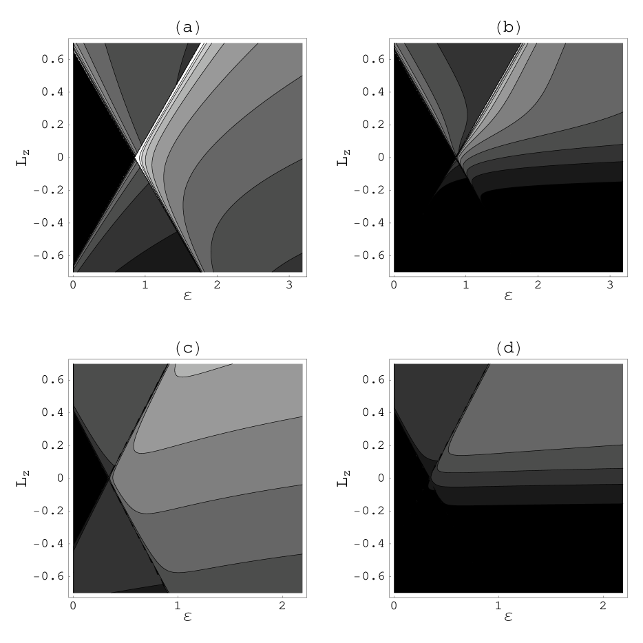
Figure 11: Contours of $\tilde{f}_{m}$, given by (46), for $m=2$, $B_{1}=0.1$ and (a) $\alpha=1$; (b) $\alpha=10$. Moreover, it is plotted the case $m=3$ with $B_{1}=0.2$ and (c) $\alpha=1$; (d) $\alpha=10$. Larger values of the DF corresponds to lighter zones.

5 Concluding Remarks

We have obtained a set of models for axisymmetric flat galaxies, by superposing members belonging to the generalized Kalnajs discs family. The mass distribution of each model (labeled through the parameter $m=2,3,\ldots$), described by (10), is maximum at the center and vanishes at the edge, in concordance with a great variety of galaxies. Moreover, the mass density can be expressed as a function of the gravitational potential (see equation (22)), which makes possible to derive, analytically, the equilibrium DFs describing the statistical features of the models.

These models have also interesting features concerning with the interior kinematical behavior. On one hand, we showed that for some values of $B_{1}$, the circular velocity has a behavior very similar to that seen in many discoidal galaxies. This is a very relevant fact, which suggests that it is not always necessary to introduce the hypothesis of dark matter halos (or MOND theories) in order to describe adequately a variety of rotational curves. On the other hand, the analysis of epicyclic and vertical frequencies, associated to quasi-circular orbits, reveals that the models are stable under radial perturbations but unstable under vertical disturbances. With regard to the motion of test particles around the models formulated here, we found that the behavior of disc-crossing orbits is similar to that seen in the generalized Kalnajs family. However, for certain values of the parameter $B_{1}$, the Poincaré surface of section reveals that one can suggest the existence of a (non analytical) third integral of motion.

On the other hand, we find two kinds of equilibrium DFs for the models. Such two-integral DFs can be formulated, at first, as functionals of the Jacobi’s integral, as it was sketched in the formalism developed by Kalnajs (1976). This class of DFs essentially describes systems which rotational state, in average, behaves as a rigid body. Then, we use the procedure introduced by Dejonghe (1986), obtaining DFs which represents systems with a mean rotational state consistent with the maximum entropy principle and, therefore, more probable than the first ones. The statements exposed above suggest that the family presented here, can be considered as a set of realistic models that describes satisfactorily a great variety of galaxies.

6 Acknowledgments

J. R-C. thanks the financial support from Vicerrectoría Académica, Universidad Industrial de Santander.

References

- Arfken (2005) Arfken G. & Weber H., 2005, Mathematical Methods for Physicists. 6th Ed., Academic Press.
- Bagin (1987) Bagin V. M., 1972, Astron. Zhur., 49, 1249.
- Binney & Tremaine (1987) Binney, J. and Tremaine, S., 1987, Galactic Dynamics. Princeton University Press, Princeton, N. J.
- Brandt & Belton (1962) Brandt, J. C. and Belton, M. J. S., 1962, Ap. J., 136, 352
- Dejonghe (1986) Dejonghe, H., 1986, Phys. Rep., 133 (3& 4), 217.
- Evans (1993) Evans N. W., 1993, MNRAS, 260, 191.
- Evans (1994) Evans N. W., 1994, MNRAS, 267, 333.
- Fricke (1962) Fricke, W. , 1952, Astron. Nachr., 280, 193-216.
- González & Reina (2006) González, G. A. and Reina, J. I. 2006, MNRAS, 371 (4), 1873-1876.
- Hunter (1963) Hunter, C., 1963, MNRAS, 126, 299.
- Hunter & Quian (1993) Hunter C. & Quian E. 1993, MNRAS, 262 , 401-428.
- Jiang (2000) Jiang Z., 2000, MNRAS, 319, 1067.
- Jiang & Moss (2002) Jiang Z. & Moss D., 2002, MNRAS, 331, 117.
- Jiang & Ossipkov (2006) Jiang Z. & Ossipkov L., 2006, Astron. Astroph. Trans., 25, 213.
- Jiang & Ossipkov (2007) Jiang Z. & Ossipkov L., 2007, MNRAS, 379 (3),1133-1142.
- Kalnajs (1972) Kalnajs, A. J., 1972, Ap. J., 175, 63.
- Kalnajs (1976) Kalnajs, A. J., 1976, Ap. J., 205, 751.
- Kutuzov (1995) Kutuzov S. A., 1995, Astron. Astroph. Trans., 7, 191.
- Kutuzov (1980) Kutuzov S. A., Ossipkov L. P., 1980, Astron. Zhur., 57, 28.
- Kutuzov (1986) Kutuzov S. A., Ossipkov L. P., 1986, Translated from Astrofizika, 25(3), 545-558.
- Kutuzov (1988) Kutuzov S. A., Ossipkov L. P., 1988, Astron. Zhur., 65, 468.
- Kuzmin (1956) Kuzmin, G., 1956, Astron. Zh., 33, 27.
- Linden-Bell (1962) Linden-Bell, D., 1962, MNRAS, 123, 447-458.
- Miyamoto (1971) Miyamoto M., 1971, Publ. Astron. Soc. Japan, 23, 21.
- Miyamoto & Nagai (1975) Miyamoto M. & Nagai R., 1975, Publ. Astron. Soc. Japan, 27, 533.
- Miyamoto & Nagai (1976) Nagai R. & Miyamoto M., 1976, Publ. Astron. Soc. Japan, 28, 1.
- Pedraza, Ramos-Caro & González (2008) Pedraza J. F., Ramos-Caro J. & González G. A., 2008, submitted to MNRAS.
- Ramos-Caro, López-Suspez & González (2008) Ramos-Caro J., López-Suspez F. & González G. A., 2008, MNRAS, 386, 440-446.
- Schmith (1956) Schmith, M., 1956, Bull. Astron. Inst. Neth, 13, 15.
- Toomre (1963) Toomre, A., 1963, Ap. J., 138, 385.
- Toomre (1964) Toomre, A., 1964, Ap. J., 139, 1217
- Wyse & Mayall (1942) Wyse, A. B. and Mayall, N. U., 1942, Ap. J., 95, 24