Heat conduction in a 1D harmonic chain with three dimensional vibrations

Abstract

We study vibrational energy transport in a quasi 1-D harmonic chain with both longitudinal and transverse vibrations. We demonstrate via both numerical simulation and theoretic analysis that for 1-D atomic chain connected by 3D harmonic springs, the coefficient of heat conduction changes continuously with its lattice constant, indicating the qualitative difference from the corresponding 1-D case where the coefficient is independent of the lattice constant.

1 Introduction

Heat conduction in low dimensional systems (less than three dimension) has been attracting increasing attention in the past decade[1]. From the fundamental point of view, one would like to know whether the fundamental transport theory for bulk material, such as the Fourier law of heat conduction, is still valid for such low dimensional systems. In fact, the question is not trivial, as there is still no rigorous proof available so far. From application point of view, it is an indispensable question to understand the heat conduction properties of the nanoscale materials before they are put into application [2].

In order to understand the underlying physical mechanism of heat conduction in one dimensional (1D) systems, different lattice models with and without on-site (pinning) potential have been used, such as the Fermi-Pasta-Ulam model [3] without on-site potential, the Frenkel Kontorova model[4], and the $\phi^{4}$ model with on-site potential [5]. With these models, the roles of anharmonicity and the on-site potential in heat conduction in 1D systems have been nicely demonstrated. For example, in the system without on-site potential, a size-dependent thermal conductivity has been observed [3] due to a superdiffusive motion of phonons [6]. In the system with on-site potential, the scattering from on-site potential makes phonon transport diffusively, leading to a size-independent thermal conductivity. Considering the fact that in the 1D models, the lattice is restricted to longitudinal vibration only, i.e., the transverse motions have been completely ignored, we conclude that these 1D models are too simple to be used for modelling heat conduction in realistic nanostructures, such as nanotube and nanowires.

Indeed, the heat conduction behavior changes when the transverse vibrations are considered. In a recent work, Wang and Li[7] considered a model of quasi 1D chain connected by 2D spring with a bending angle interaction. The lattices are allowed to vibrate in longitudinal as well as in one transverse direction. The results show that for a fixed lattice constant, the anomalous heat conduction coefficient $\kappa(N)$ changes from a logarithmic divergence with system size $N$, i.e, $logN$ for large transverse coupling, to a $1/3$ power law divergence, $N^{1/3}$, at intermediate coupling, and then to a $2/5$ power law divergence, $N^{2/5}$ at low temperatures and weak coupling. The results are mainly due to the mode coupling between the longitudinal modes and transverse modes.

In this paper, we study the quasi 1D chain with motion in both the longitudinal direction and the two transverse directions. Namely, the lattices can vibrate in all three directions, which is more closer to real nano-scale quasi 1D systems. For simplicity, we call our system a 3D harmonic chain. To be more practical, we will not going to discuss the thermodynamic limit (length goes to infinity) as most of the nanoscale systems are of finite length. Instead, we shall focus on the effect of the lattice constant. The model discussed by Wang and Li[7] can be considered as a simplified polymer chain, while the model studied in our current paper can be considered as simplified nanotube or nanowire model.

We shall demonstrate soon that, in 1D case, the lattice constant does not play any role when the atoms can be considered as moving around its equilibrium; while in 3D case, the situation is totally different and the lattice constant will influence the heat conduction. It goes back to the 1D case when the lattice constant $a\rightarrow\infty$.

2 Model and numerical results

The 3D harmonic chain is coupled with the Nose-Hoover thermostats [8] on the first and last particle, keeping them at temperature $T_{h}$ and $T_{l}$, respectively. The Hamiltonian is

$$H=\frac{1}{2}\sum_{i}p_{ix}^{2}+p_{iy}^{2}+p_{iz}^{2}+\frac{1}{2}\sum_{i}(|{\bf r}_{i+1}-{\bf r}_{i}|-a)^{2},$$ (1)

where $a$ is the lattice constant, ${\bf r}_{i}=(ia+x_{i},y_{i},z_{i})$, and $x_{i},y_{i},z_{i}$ are the displacements from the equilibrium position $(ia,0,0)$. The motion of the particles satisfy the canonical equations $\dot{q}_{iw}=\partial H/\partial p_{iw}$ and $\dot{p}_{iw}=-\partial H/\partial q_{iw}$ with $w=x,y,z$, respectively, and $i=2,3,\cdots,N-1$. The left and right heat baths are described respectively by the equations,

$$\dot{\xi}_{h}=\frac{1}{3T_{h}}(\dot{q}_{1x}^{2}+\dot{q}_{1y}^{2}+\dot{q}_{1z}^{2})-1,$$

$$\dot{\xi}_{l}=\frac{1}{3T_{l}}(\dot{q}_{Nx}^{2}+\dot{q}_{Ny}^{2}+\dot{q}_{Nz}^{2})-1,$$ (2)

The equations of the motion for the first and last particle are $\dot{q}_{1w}=\partial H/\partial p_{1w}$, $\dot{p}_{1w}=-\partial H/\partial q_{1w}-\xi_{h}p_{1w}$, $\dot{q}_{Nw}=\partial H/\partial p_{Nw}$, and $\dot{p}_{Nw}=-\partial H/\partial q_{Nw}-\xi_{l}p_{Nw}$ with $w=x,y,z$, respectively. Substituting Eq. (1) into the canonical equations we can get the expressions of $\dot{p}_{ix}$, $\dot{p}_{iy}$ and $\dot{p}_{iz}$ as follows

$$\dot{p}_{ix} = (1-\frac{a}{d_{i+1}})(a+\Delta x_{i+1})-(1-\frac{a}{d_{i}})(a+\Delta x_{i}),$$

$$\dot{p}_{iy} = (1-\frac{a}{d_{i+1}})\Delta y_{i+1}-(1-\frac{a}{d_{i}})\Delta y_{i},$$ (3)

$$\dot{p}_{iz} = (1-\frac{a}{d_{i+1}})\Delta z_{i+1}-(1-\frac{a}{d_{i}})\Delta z_{i},$$

where $d_{i+1}=\sqrt{(a+\Delta x_{i+1})^{2}+(\Delta y_{i+1})^{2}+(\Delta z_{i+1})^{2}}$, $\Delta x_{i+1}=x_{i+1}-x_{i}$, $\Delta y_{i+1}=y_{i+1}-y_{i}$, and $\Delta z_{i+1}=z_{i+1}-z_{i}$.

Re-scaling $q_{iw}$ and $p_{iw}$ as $q^{\prime}_{iw}=q_{iw}/a$ and $p^{\prime}_{iw}=p_{iw}/a$ with $w=x,y,z$, respectively, Eq. (2) becomes

$$\dot{p^{\prime}}_{ix} = (1-\frac{1}{d^{\prime}_{i+1}})(1+\Delta x^{\prime}_{i+1})-(1-\frac{1}{d^{\prime}_{i}})(1+\Delta x^{\prime}_{i}),$$

$$\dot{p^{\prime}}_{iy} = (1-\frac{1}{d^{\prime}_{i+1}})\Delta y^{\prime}_{i+1}-(1-\frac{1}{d^{\prime}_{i}})\Delta y^{\prime}_{i},$$ (4)

$$\dot{p^{\prime}}_{iz} = (1-\frac{1}{d^{\prime}_{i+1}})\Delta z^{\prime}_{i+1}-(1-\frac{1}{d^{\prime}_{i}})\Delta z^{\prime}_{i},$$

where $d^{\prime}_{i+1}=\sqrt{(1+\Delta x^{\prime}_{i+1})^{2}+(\Delta y^{\prime}_{i+1})^{2}+(\Delta z^{\prime}_{i+1})^{2}}$. The heat bath Eqs. (2) is re-scaled as:

$$\dot{\xi}_{h}=\frac{1}{3T^{\prime}_{h}}(\dot{q^{\prime}}_{1x}^{2}+\dot{q^{\prime}}_{1y}^{2}+\dot{q^{\prime}}_{1z}^{2})-1,$$

$$\dot{\xi}_{l}=\frac{1}{3T^{\prime}_{l}}(\dot{q^{\prime}}_{Nx}^{2}+\dot{q^{\prime}}_{Ny}^{2}+\dot{q^{\prime}}_{Nz}^{2})-1.$$ (5)

where $T^{\prime}_{h,l}=T_{h,l}/a^{2}$. This means that the equations $\dot{p}_{1w}$ and $\dot{p}_{Nw}$ for the boundary particles are invariant providing that the temperature of the two heat baths are re-scaled as mentioned above. This is interesting. It indicates that in our system, the model with twice smaller lattice constant is identical with the one with four times smaller temperature.

For the case of fixed temperatures $T_{h}$ and $T_{l}$, the re-scaling of $q_{1w}$ and $q_{Nw}$ will cause different $\dot{\xi}_{h}$ and $\dot{\xi}_{l}$, namely, the effect of lattice constant will show up through the heat baths and result in different behaviors of heat conduction. This can be understood like this. For a given $T_{h}$ and $T_{l}$, the average of the amplitude of $\dot{q}_{iw}$ are fixed for the heat bath particles. Therefore, larger $a$ means a relatively smaller $q^{\prime}_{iw}$. Making a Taylor expansion of $d^{\prime}_{i+1}$ with respect to $\Delta x_{i}^{\prime},\Delta y_{i}^{\prime}$, and $\Delta z_{i}^{\prime}$, from Eq. (2) we see that $\dot{p^{\prime}}_{ix}$ is proportional to the first order of $\Delta x^{\prime}_{i}$ and $\dot{p^{\prime}}_{iy}$ and $\dot{p^{\prime}}_{iz}$ are proportional to the second order of $\Delta x^{\prime}_{i}$. Therefore, smaller $q^{\prime}_{iw}$ or larger $a$ will make the transverse motion negligible, indicating that we may observe a harmonic motion for the larger $a$. Generally, with the decrease of $a$, the transverse motion will become more and more important and thus influence the heat conduction more. When $q^{\prime}_{iw}$ reaches the magnitude of unity or of lattice constant, the heat conduction will be saturated, thus we may observe a platform for small enough $a$.

3 Heat conductivity versus system size and lattice constant

The temperature of the i’th lattice is defined as $T(i)=(\langle p_{ix}^{2}\rangle+\langle p_{iy}^{2}\rangle+\langle p_{iz}^{2}\rangle)/3$ and the heat flux along the chain in stationary state is defined as $J=\langle p_{ix}\frac{\partial V_{i+1,i}}{\partial x_{i}}+p_{iy}\frac{\partial V_{i+1,i}}{\partial y_{i}}+p_{iz}\frac{\partial V_{i+1,i}}{\partial z_{i}}\rangle$ where $V_{i+1,i}=\frac{1}{2}(|{\bf r}_{i+1}-{\bf r}_{i}|-a)^{2}$. From the Fourier law $J=-\kappa\nabla T$, the heat conductivity can be expressed as

$$\kappa(N)=J(N-1)/(T_{h}-T_{l}).$$ (6)

For fixed $T_{h}$ and $T_{l}$, $JN$ can be used to represent the $\kappa$. For a momentum conservative 1D lattice, it is found that the heat conduction is anomalous[1, 3, 6], namely, the heat conductivity depends on the system size as

$$\kappa(N)\sim N^{\beta},$$ (7)

where $\beta$ varies from system to system. In this paper, we study the dependence of $\beta$ on the lattice constant $a$. For comparison, we study two concrete cases: a relatively high temperature regime and a relatively low temperature regime. For the low temperature case, we take $T_{h}=0.07$ and $T_{l}=0.05$, thus the system temperature defined by $T\equiv(T_{h}+T_{l})/2$ is $T=0.06$. For high temperature case, we take $T_{h}=0.3$ and $T_{l}=0.2$, thus the system temperature is $T=0.25$ which is about four times higher than the previous one. The results are shown in Fig.1(a) and (b). Our numerical simulations reveal that $NJ$ increases with $N$ by different scaling for different $a$ and different temperatures $T_{h/l}$.

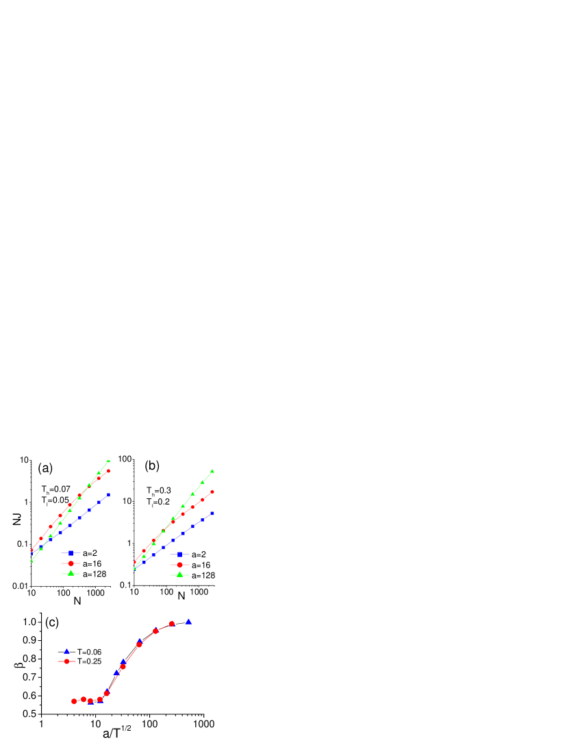
Figure 1: $NJ$ versus $N$ for different temperatures. (a) $T_{h}=0.07$ and $T_{l}=0.05$, thus $T\equiv(T_{h}+T_{l})/2=0.06$. (b) $T_{h}=0.3$ and $T_{l}=0.2$, thus $T\equiv(T_{h}+T_{l})/2=0.25$. (c) $\beta$ versus $a/\sqrt{T}$.

As we have pointed out early that, in the dimensionless Hamiltonian, the system for different $a$ and different heat bath temperatures can be equivalent, therefore, in Fig 1(c) we draw $\beta$ versus the quantity $a/\sqrt{T}$.

It is quite obvious that two sets of data from Fig.1(a) and (b) almost overlap with each other in Fig.1(c). We have also checked other pairs of $T_{h}$ and $T_{l}$ ( such as $T_{h}=0.1$ and $T_{l}=0.005$) and found that they also overlap with each other. From Fig.1(c) it is easy to see that $\beta$ goes to unity for $a/\sqrt{T}>300$, indicating the large lattice constant or very low temperature makes the 3D chain equivalent to a 1D harmonic chain. Moreover, $\beta$ drops with the decrease of $a$ or increase of temperature, and reaches a platform for $a/\sqrt{T}\leq 15$, confirming the theoretic analysis of the previous section.

We have checked the behaviors of the particles and found that the particles oscillate around their equilibrium positions and can be considered as local when $a$ is relatively large and their oscillation can not be considered as local when $a$ is in the range of platform. For the relatively small $a$, it is possible for the particle to move to the area with $|x_{i}|>a$. Figure 2 shows the snapshots of the deviation of particle’s positions from their equilibriums. It can be seen that the positions at $i=17-23$ satisfy $|x_{i}|>a(=2)$, and the similar situation occurs in Fig. 2(b) for $i=12$. This kind of non-local behavior causes the platform. High environment temperature causes large deviation of $|x_{i}|$ from $a$, hence results in a larger platform as is shown in Fig. 1(c).

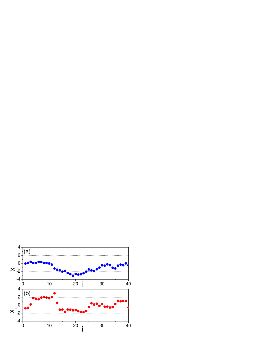
Figure 2: Snapshots of $x_{i}$, the deviation from the equilibrium position, for $a=2$. (a) $T_{h}=0.07$ and $T_{l}=0.05$; (b) $T_{h}=0.3$ and $T_{l}=0.2$.

4 Anomalous energy diffusion

In order to confirm further the influence of lattice constant on the heat conduction in the 3D harmonic chain, we study the diffusion for different $a$. First, we let the two heat baths have the same temperature and let the chain run enough time to achieve the equilibrium. Then we give a pulse of energy, which is larger than the energy of the equilibrium state, at the middle particle of the chain and investigate how the pulse of energy spreads to the other part of the chain. Figure 3 shows the result for $T_{l}=T_{h}=0.2$, $N=201$, and the results are obtained by averaging over $10^{3}$ realizations where the initial pulse of five times the average momentum is added at the particle $i=101$, i.e., at $t=0$ we change the velocity of the middle particle to $5$ times of its previous value. Figure 3(a) and (a’) denote the snapshot at time $t=1$, (b) and (b’) at $t=3$, (c) and (c’) at $t=10$, (d) and (d’) at $t=30$, and (e) and (e’) at $t=100$, and the left panels represent the situation of $a=2$ and the right panels represent the situation of $a=128$.

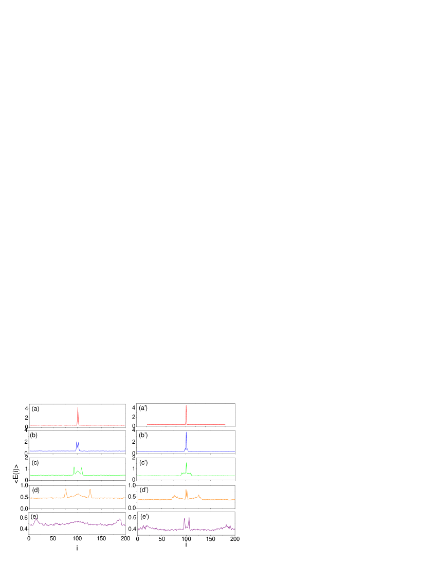
Figure 3: Snapshots of $\langle E(i)\rangle$ at different times for $N=201$, $T=0.2$, and the initial pulse $p1_{101x}(0)=5p_{101x}(0)$, $p1_{101y}(0)=5p_{101y}(0)$, $p1_{101z}(0)=5p_{101z}(0)$ is added at the particle $i=101$ at $t=0$ where the left panels represent the situation of $a=2$, the right panels represent the situation of $a=128$, and (a) and (a’) denote the snapshot at time $t=1$, (b) and (b’) at $t=3$, (c) and (c’) at $t=10$, (d) and (d’) at $t=30$, and (e) and (e’) at $t=100$.

Obviously, the left panels of Figure 3 are different from the right panels, reflecting the influence of the lattice constant. Ref. [6] gives an approach to measure the energy diffusion by the formula, $\sigma^{2}(t)=\frac{\int(E(x,t)-E_{0})(x-x_{0})^{2}dx}{\int(E(x,t)-E_{0})dx},$ where $E(x,t)$ is the energy distribution at time $t$, $x_{0}$ is the position of initial energy pulse at $t=0$, $E_{0}$ is the energy of the equilibrium state with temperature $T$. However, in the 3-D case, this approach does not work very well because the energy $E(x,t)$ fluctuates around $E_{0}$ and makes the diffusion contributions in the integral of this equation cancel each other.

A correct way is to make the diffusion contributions always positive, i.e., make the numerator in this equation positive at each position $x$. Ref.[9] points out recently that, if the pulse is very small and is initially localized at $i=i_{0}$, the energy diffusion can be given by

$$\sigma^{2}(t)=\sum_{i}(i-i_{0})^{2}\delta_{(2)}(i,t),$$ (8)

where $\delta_{(2)}(i,t)=(\delta v_{i}(t))^{2}$ in the 1D case. Here we extend this approach to the 3D case and take

$$\delta_{(2)}(i,t) = (\delta p_{ix}(t))^{2}+(\delta p_{iy}(t))^{2}+(\delta p_{iz}(t))^{2}$$ (9)

$$+(\delta x_{i}(t))^{2}+(\delta y_{i}(t))^{2}+(\delta z_{i}(t))^{2}.$$

That is, $\sigma^{2}(t)$ measures the total energy variation caused by the diffusion of the pulse. In numerical simulations, after the system arrives at the equilibrium we record the time as $t=0$ and copy all the variables ${\bf x}_{i}$ and ${\bf p}_{i}$ to a new set of variables ${\bf x1}_{i}$ and ${\bf p1}_{i}$ except the middle one ${\bf p1}_{101}=1.5{\bf p}_{101}$ where 1.5 chosen so as to make the initial pulse small enough. Hence, we have two set of systems (${\bf x}_{i},{\bf p}_{i}$) and (${\bf x1}_{i},{\bf p1}_{i}$) with ${\bf x1}_{i}={\bf x}_{i}$, ${\bf p1}_{i}={\bf p}_{i}$ for $i\not=i_{0}$ and ${\bf x1}_{i_{0}}={\bf x}_{i_{0}}$, ${\bf p1}_{i_{0}}=1.5{\bf p}_{i_{0}}$ at $t=0$. As time goes on, the corresponding variables will gradually become different because of the diffusion of the pulse. Then, we can obtain a nonzero $\delta p_{ix}(t)=p1_{ix}(t)-p_{ix}(t)$, $\delta x_{i}(t)=x1_{i}(t)-x_{i}(t)$, and so on. In this way, we can find the relation $\sigma^{2}(t)\sim t^{\alpha}$ through Eqs. (9) and (8). Figure 4(a) shows the result for three typical values of $a$ at $T=0.05$, which are obtained by averaging over $10^{3}$ realizations. The line with “squares” denotes the case of $a=2$, the line with “circles” the case of $a=16$, and the line with “triangles” the case of $a=128$. We have the similar situations for other $a$. The slopes of the lines in Fig.4(a) give the exponent $\alpha$.

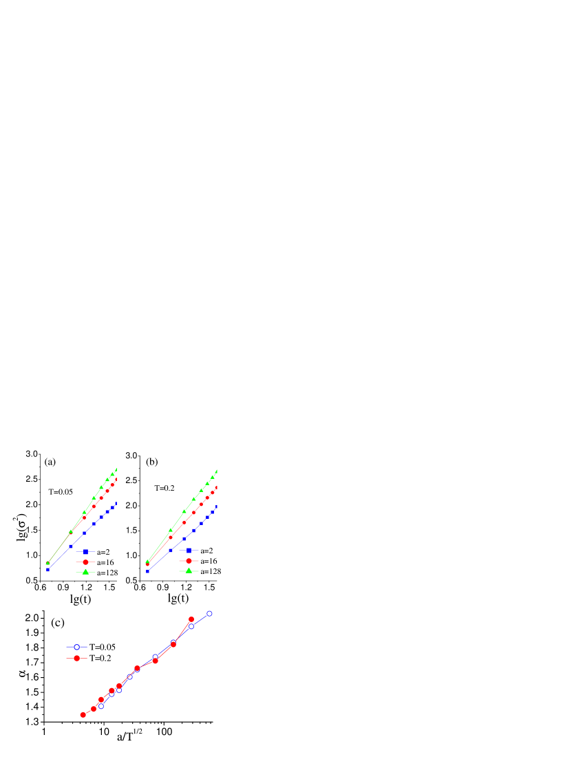
Figure 4: Three typical situations of $\sigma$ versus $t$ for $T=0.05$ (a) and $T=0.2$ (b). We have taken an ensemble average over $10^{3}$ realizations. (c) $\alpha$ versus $a/\sqrt{T}$ for $T=0.05$ and $T=0.2$.

Fig. 4(b) show the case of $T=0.2$.

For the same reason as in Fig 1, we also draw here $\alpha$ versus $a/\sqrt{T}$ in 4(c). The two sets of date overlap quite well. More interestingly, the Fig. 4(c) clearly indicates that

$$\alpha=A+B\log_{10}\left(a/\sqrt{T}\right),$$ (10)

where $A\approx 1.138$ and $B\approx 0.325$ are two constants. Why the exponent of superdiffusion is related to the lattice constant $a$ and temperature $T$ in such a relation deserves further investigation.

5 Conclusions and discussions

In summary, we have studied heat conduction in a quasi 1-D system with 3D vibration. For finite length (around $1,000$ units or, for a typical crystal atom chain, $100$ nanometers), the heat conduction is anomalous and energy diffusion is superdiffusive. Moreover, we have demonstrated that both the anomalous heat conduction exponent $\beta$ and the anomalous diffusion exponent $\alpha$ depends on the dimensionless quantity, $a/\sqrt{T}$. In particular, we found that $\alpha=A+B\ln(a/\sqrt{T})$ for reasons to be further investigated.

We should emphasize that the results obtained in this paper are for a finite size system, which is more appropriate as the nanoscale systems are always of finite size. Therefore, the obtained results may shed lights in understanding heat conduction in nanoscale structures, especially in networked structure [10]. As the quasi 1D systems such as the nanowires and nanotubes can be fabricated easily these days, it is therefore of great interest to do the measurement on the size dependent thermal conductivity of these systems and to compare with the results presented.

Acknowlegments

This work was partly supported by the National Science Foundation of China under Grant No. 10775052 and No. 10635040 (ZL) and a Faculty Research Grant of National University of Singapore.

References

- [1] F. Bonetto, J. Lebowitz, and L. Rey-Bellet, in Mathematical Physics 2000, ed. A. Fokas et al. (Imperial College Press, London, 2000) p. 128; D. G. Cahill, W. K. Ford, K. E. Goodson, G. D. Mahan, A. Majumdar, H. J. Maris, R. Merlin and S. R. Phillpot: J. Appl. Phys. 93 (2003) 793.
- [2] M. S. Gudiksen, L. J. Lauhon, J. Wang, D. C. Smith, and C. M. Lieber: Nature 415 (2002) 617; G. Chen and C. L. Tien: J. Appl. Phys. 74 (1993) 2167; K. E. Goodson and Y. S. Ju: Anuu. Rev. Mater. Sci. 29 (1999) 261.
- [3] H. Kaburaki and M. Machida: Phys. Lett. A 181 (1993) 85; S. Lepri, R. Livi, and A. Politi: Phys. Rev. Lett. 78 (1997) 1896; A. Fillipov, B. Hu, B. Li, and A. Zeltser: J. Phys. A 31 (1998) 7719; S. Lepri: Phys. Rev. E 58 (1998) 7165; K. Aoki and D. Kusnezov: Phys. Rev. Lett. 86 (2001) 4029; A. Pereverzev: Phys. Rev. E 68 (2003) 056124.
- [4] B. Hu, B. Li, and H. Zhao: Phys. Rev. E 57 (1998) 2992; A. V. Savin and O. V. Gendelman: Phys. Rev. E 67 (2003) 041205.
- [5] B. Hu, B. Li, and H. Zhao: Phys. Rev. E 61 (2000) 3828; K. Aoki and D. Kusnezov: Phys. Lett. A 265 (2000) 250.
- [6] B. Li and J. Wang: Phys. Rev. Lett. 91 (2003) 044301; B. Li, J. Wang, L. Wang, and G. Zhang: Chaos 15 (2005) 015121; G. Zhang and B. Li: J. Chem. Phys. 123 (2005) 014705.
- [7] J.-S Wang and B. Li, Phys. Rev. Lett. 92, 074302 (2004); Phys. Rev. E 70, 021204 (2005).
- [8] S. Nose: J. Chem. Phys. 81 (1984) 511; W. G. Hoover: Phys. Rev. A 31 (1985) 1695.
- [9] P. Cipriani, S. Denisov, and A. Politi: Phys. Rev. Lett. 94 (2005) 244301.
- [10] Z. Liu and B. Li: Phys. Rev. E 76, (2007) 051118.