Theory of the spin nematic to spin-Peierls quantum phase transition
in ultracold spin-1 atoms in optical lattices

Abstract

We present a theory of the anisotropy tuned quantum phase transition between spin nematic and spin-Peierls phases in $S=1$ systems with significant bi-quadratic exchange interactions. Based on quantum Monte Carlo studies on finite size systems, it has been proposed that this phase transition is second order with new deconfined fractional excitations that are absent in either of the two phases. The possibility of a weak first order transition, however, cannot be ruled out. To elucidate the nature of the transition, we construct a large-$N$ SO(3$N$) model for this phase transition and find in the $N\to\infty$ limit that the transition is generically of first order. Furthermore, we find a critical point in the one-dimensional (1D) limit, where two transition lines, separating spin-nematic, ferromagnetic, and spin-Peierls phases, meet. Our study indicates that the spin-nematic phase is absent in 1D, while its correlation length diverges at the critical point. Predictions for ²³Na atoms trapped in an optical lattice, where the nematic to spin-Peierls quantum phase transition naturally arises, are discussed.

I Introduction

Conventional Landau-Ginzburg theory describes continuous phase transitions by fluctuations of an order parameter. A nonzero value of the order parameter signals spontaneous symmetry breaking and the presence of an ordered phase. Moreover, if several distinct ordered ground states are possible, Landau-Ginzburg theory generically predicts that ordered phases with unrelated broken symmetries are separated by either intervening phases or a first order phase boundary. In the simplest case, this is illustrated by the free energy for two independent order parameters $\phi_{1}$ and $\phi_{2}$ as Chaikin and Lubensky (2005)

$$f=\frac{r}{2}(\phi_{1}^{2}+\phi_{2}^{2})-\frac{g}{2}(\phi_{1}^{2}-\phi_{2}^{2})+u_{1}\phi_{1}^{4}+u_{2}\phi_{2}^{4}+2u_{12}\phi_{1}^{2}\phi_{2}^{2}.$$ (1)

Here, a direct second-order transition in the $r$-$g$ parameter space between phases with either nonzero $\phi_{1}$ or $\phi_{2}$ requires fine tuning such that $u_{1}u_{2}=u^{2}_{12}$ is satisfied.

Recently, a theory of critical phase transitions has been proposed that reaches beyond the Landau-Ginzburg paradigm and allows direct continuous transitions between distinct broken-symmetry phases. Senthil et al. (2004, 2004) In this theory, the relevant degrees of freedom are described in terms of fields that carry fractional quantum numbers and become deconfined only at the critical point. In particular, it was argued that a direct continuous transition from a valence bond solid (VBS) to a Néel phase Senthil et al. (2004, 2004) or a spin-nematic phase Harada et al. (2007); Grover and Senthil (2007) falls into this class of phase transitions. For this reason the search for such deconfined critical phenomena (DCP) in simple model systems has attracted much attention.

Several systems have been studied up to now. Based on quantum Monte Carlo simulations on the two-dimensional spin-1/2 Heisenberg model with an additional four-spin interaction (“$JQ$ model”) the phase transition between a Néel ordered state and a VBS appears to be consistent with the deconfined critical scenario. Sandvik (2007); Melko and Kaul (2008) This, however, has been disputed by other numerical studies Kuklov et al. (2008); Jiang et al. (2007); Kuklov et al. (2006) that support a weakly first order transition. Another candidate system is the $Sp(4)$-Heisenberg model on a square lattice, which describes spin-3/2 cold atom systems and has also been conjectured to harbor a direct second-order transition between a Néel and a VBS state. Qi and Xu (2008)

The present approach focuses on the anisotropic bilinear bi-quadratic spin-1 Heisenberg model (“$JK$ model”) on a square lattice

$$H = \sum_{i}\big{[}J{\bf S}_{i}\cdot{\bf S}_{i+x}+K\big{(}{\bf S}_{i}\cdot{\bf S}_{i+x}\big{)}^{2}\big{]}$$ (2)

$$+\lambda\sum_{i}\big{[}J{\bf S}_{i}\cdot{\bf S}_{i+y}+K\big{(}{\bf S}_{i}\cdot{\bf S}_{i+y}\big{)}^{2}\big{]}$$

where the exchange integrals for neighboring spins in $y$ direction are reduced by an anisotropy parameter $\lambda$ (i.e., $J\rightarrow\lambda J$ and $K\rightarrow\lambda K$ on $y$ bonds). For $\lambda=0$, this Hamiltonian describes decoupled spin chains, while for $\lambda=1$ the full square lattice symmetry is recovered. The parameter range of interest is specified by $K<J<0$, which is also thought to be the natural range for ${}^{23}\text{Na}$ atoms in an optical lattice. Yip (2003); Imambekov et al. (2003) In this range the quadratic term favors ferromagnetic order, while the quartic term prefers the formation of singlet bonds. This competition is solved in two dimensions ($\lambda=1$) by having a spin-nematic ground state (which breaks spin-rotational symmetry but preserves time-reversal symmetry $\langle{\bf S}_{i}\rangle$ = 0) and in one dimension ($\lambda=0$) by forming a dimerized ground state (which breaks translational invariance). Imambekov et al. (2003); Yip (2003); Harada et al. (2007); Läuchli et al. (2006); Lewenstein et al. (2007); Podolsky and Demler (2005) When the anisotropy parameter is continuously changed between 1 and 0, quantum Monte Carlo studies by Harada et al. Harada et al. (2007) suggest that the system undergoes a Landau-forbidden direct second-order transition between the nematic and the dimer phases, which further motivated a recently developed continuum theory for the nematic-dimer phase transition based on DCP. Grover and Senthil (2007) However, because of significant finite-size effects, they were unable to rule out a weak first-order transition or the existence of two successive phase transitions. Harada et al. (2007)

In this paper, we examine the nematic-dimer phase transition in anisotropic spin-1 systems using two complementary approaches. The first approach is based on the bond operator formalism introduced by Chubukov Chubukov (1991) and is particularly suited for studying the dimer phase as pairs of neighboring spins are described by common bosonic bond operators. Taking the classical limit of this approach by neglecting all quantum fluctuations, one can already obtain a good overview over the $JK$ model. Complementary to the bond operator method, we then construct an SO($3N$) model and study its large-$N$ limit ($N=1$ is the physical limit). This approach explicitly takes the disordering effects of zero-point fluctuations into account. For $N\rightarrow\infty$ we find that a first-order phase boundary separates the spin nematic from gapped spin-liquid phases except at special SU($3N$) symmetric points, where the transition becomes second order. In the 1D ($\lambda=0$) limit, the existence of the spin-nematic phase has been studied extensively but remains elusive. Chubukov (1991); Buchta et al. (2005); Rizzi et al. (2005); Rossini et al. (2005) In this limit, we find a critical point at $J=K<0$ where spin-nematic, ferromagnetic and spin-Peierls correlation functions diverge. The spin nematic phase, however, does not exist in a finite parameter range near $J=K<0$ at $\lambda=0$. Finally, predictions for ²³Na atoms in an optical lattice, where the nematic to dimer quantum phase transition naturally arises, are presented.

II Spin-$1$ bond operator model

To gain a simple understanding of the anisotropic $JK$ model of Eq. (2), consider the classical limit of the bond operator model following Chubukov Chubukov (1991). Grouping the $N_{s}$ sites of the square lattice into $N_{s}/2$ bonds in a columnar pattern, we may reformulate the $JK$ model in terms of bosonic operators on these bonds that create and annihilate singlets $|00\rangle=\hat{s}^{\dagger}|0\rangle$, triplets $|1,m_{t}\rangle=\hat{t}_{m_{t}}^{\dagger}|0\rangle$ (where $m_{t}=0,\pm 1$), and quintuplets $|2,m_{q}\rangle=\hat{q}^{\dagger}_{m_{q}}|0\rangle$ (where $m_{q}=0,\pm 1,\pm 2$). A constraint of one boson per site is then necessary to stay within the physical Hilbert space. Allowing the bosons to completely condense (as in Bogoliubov theory) then produces a simple phase diagram based on the energy of different possible condensates.

To carry out such program, we must first re-construct the spin Hamiltonian of Eq. (2) in terms of the above-introduced bosons. On a given bond $\ell=(i,i+\hat{x})$, it is easier to work with the generators $\vec{L}_{\ell}=\vec{S}_{i}+\vec{S}_{i+\hat{x}}$ and $\vec{M}_{\ell}=\vec{S}_{i}-\vec{S}_{i+\hat{x}}$ than with the spin operators directly. Direct evaluation of the matrix elements of these operators in the total spin basis of bond $\ell$ then tells us how to represent them in terms of singlet, triplet and quintuplet operators. While a little tedious, the net result is (dropping the bond labeling $\ell$):

$$\hat{L}^{z} =\sum_{m_{t}}m_{t}t^{\dagger}_{m_{t}}t_{m_{t}}+\sum_{m_{q}}m_{q}q^{\dagger}_{m_{q}}q_{m_{q}}$$ (3)

$$\hat{L}^{+} =\sqrt{2}\big{(}t^{\dagger}_{1}t_{0}+t^{\dagger}_{0}t_{-1}\big{)}+2\big{(}q^{\dagger}_{2}q_{1}+q^{\dagger}_{-1}q_{-2}\big{)}$$ (4)

$$\ \ \ \ +\sqrt{6}\big{(}q^{\dagger}_{1}q_{0}+q^{\dagger}_{0}q_{-1}\big{)}$$

$$\hat{L}^{-} =\sqrt{2}\big{(}t^{\dagger}_{0}t_{1}+t^{\dagger}_{-1}t_{0}\big{)}+2\big{(}q^{\dagger}_{1}q_{2}+q^{\dagger}_{-2}q_{-1}\big{)}$$ (5)

$$\ \ \ \ +\sqrt{6}\big{(}q^{\dagger}_{0}q_{1}+q^{\dagger}_{-1}q_{0}\big{)}$$

$$\hat{M}^{z} =\sqrt{\frac{8}{3}}\big{(}t^{\dagger}_{0}s+s^{\dagger}t_{0}\big{)}+\sqrt{\frac{4}{3}}\big{(}q^{\dagger}_{0}t_{0}+t^{\dagger}_{0}q_{0}\big{)}$$ (6)

$$\ \ \ \ +q^{\dagger}_{1}t_{1}+t^{\dagger}_{1}q_{1}+q^{\dagger}_{-1}t_{-1}+t^{\dagger}_{-1}q_{-1}$$

$$\hat{M}^{+} =-\frac{4}{\sqrt{3}}\big{(}t^{\dagger}_{1}s-s^{\dagger}t_{-1}\big{)}-2\big{(}q^{\dagger}_{2}t_{1}-t^{\dagger}_{-1}q_{-2}\big{)}$$ (7)

$$\ \ \ \ -\sqrt{2}\big{(}q^{\dagger}_{1}t_{0}-t^{\dagger}_{0}q_{-1}\big{)}-\sqrt{\frac{2}{3}}\big{(}q^{\dagger}_{0}t_{-1}-t^{\dagger}_{1}q_{0}\big{)}$$

$$\hat{M}^{-} =-\frac{4}{\sqrt{3}}\big{(}t^{\dagger}_{1}s-s^{\dagger}t_{-1}\big{)}-2\big{(}q^{\dagger}_{2}t_{1}-t^{\dagger}_{-1}q_{-2}\big{)}$$ (8)

$$\ \ \ \ -\sqrt{2}\big{(}q^{\dagger}_{1}t_{0}-t^{\dagger}_{0}q_{-1}\big{)}-\sqrt{\frac{2}{3}}\big{(}q^{\dagger}_{0}t_{-1}-t^{\dagger}_{1}q_{0}\big{)}$$

To compute the condensate energies for various phases, it is then useful to group the bosonic operators into a single vector $\vec{\psi}=(s,t_{1},t_{0},t_{-1},q_{2},...,q_{-2})$ and to express the above operators in the compact form $\hat{L}^{z}=\psi^{\dagger}_{\alpha}L^{z}_{\alpha,\beta}\psi_{\beta}$, etc. Substituting these expressions into the Hamiltonian then leaves us with the generic form

$$H=\sum_{\ell}h^{(1)}_{\alpha}\psi^{\dagger}_{\ell,\alpha}\psi_{\ell,\alpha}+\sum_{\langle\ell\ell^{\prime}\rangle}h^{(2)}_{\alpha,\beta,\gamma,\delta}(\ell,\ell^{\prime})\psi^{\dagger}_{\ell,\alpha}\psi^{\dagger}_{\ell^{\prime},\beta}\psi_{\ell^{\prime},\gamma}\psi_{\ell,\delta}$$ (9)

where $h^{(1)}$ and $h^{(2)}$ depend on $J/K$. That this Hamiltonian consists of only one-body and two-body terms results from the one boson per bond constraint. Assuming the bosons condense $\psi_{\ell,\alpha}=\langle\psi_{\ell,\alpha}\rangle+\delta\psi_{\ell,\alpha}$, we then extract the leading contribution to the condensate energy by expanding the ground-state energy to zeroth order in powers of $\delta\psi_{\ell,\alpha}$.

Four phases are of particular interest: a ferromagnetic phase with all spins pointing up, a dimerized spin-Peierls phase with a singlet on each bond, a “spin nematic” phase in which each site is in the state $|1,0\rangle$ and an antiferromagnetic phase with $|1,1\rangle$ ($|1,-1\rangle$) on the A (B) sublattice. The bosonic condensates for these idealized states are: $\langle q_{2}\rangle=1$ in the ferromagnetic phase; $\langle s\rangle=1$ in the dimer phase; $\langle q_{0}\rangle=\sqrt{2/3}$ and $\langle s\rangle=1/\sqrt{3}$ in the spin-nematic phase; and $\langle s\rangle=1/\sqrt{3}$, $\langle t_{0}\rangle=(-1)^{y}/\sqrt{2}$ and $\langle q_{0}\rangle=1/\sqrt{6}$ in the antiferromagnetic phase (the sign here alternates along a column in the columnar dimer pattern).

Using the above condensates as a guide, we construct a simple phase diagram by minimizing the condensate energy as a function of $\langle s\rangle$, $\langle t_{m_{t}}\rangle$, and $\langle q_{m_{q}}\rangle$ on at most two independent neighboring bonds (that is, we explore an 18-variational-parameter space). This approach follows that of Ref. Chubukov, 1991 in essence and can be thought of as a simple two-site clustering method. The resulting phase diagram is depicted in Fig. 1. All phases except the ferromagnetic phase have a finite dimerization due to the explicit translational symmetry breaking of this approach.

It is worth noting the finite existence of a spin-nematic phase in the one-dimensional $\lambda=0$ limit as shown in Fig. 1. This phase is not expected to survive in the presence of quantum fluctuations (finite $\delta\psi_{\ell,\alpha}$) as pointed out by Chubukov Chubukov (1991). However, the resulting phase diagram after these effects are included is not clear from this approach. The absence or presence of a (gapped) spin nematic in the 1D limit has been the focus of extensive numerical studies based on density matrix renormalization group, exact diagonalization, quantum state transfer, etc. Fáth et al. (2006); Läuchli et al. (2006); Rizzi et al. (2005); Rossini et al. (2005); Rmoero-Isart et al. (2007) This issue still remains to be settled as diverging correlation lengths near the ferromagnetic phase limit numerical approaches. We will show below that in the large-$N$ limit of the $JK$ model the spin nematic phase does not occupy a finite parameter region near the critical point $J/K=1$ for $\lambda=0$, while, approaching the critical point, spin-nematic correlations certainly diverge. This suggests that the one-dimensional spin-nematic phase vanishes even for $N=1$, although $1/N$ fluctuations may qualitatively change the universality class of the phase transition from that of the large-$N$ limit.

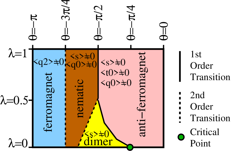
Figure 1: (Color online) Classical phase diagram. All phases are described by a finite condensate of bosonic bond operators following Chubukov (Ref. Chubukov, 1991). Note the existence of a spin-nematic phase in the one-dimensional ($\lambda=0$) limit.

III Spin-$1$ Schwinger boson model

In contrast to the bond operator approach, large-$N$ methods include the disordering effects of quantum fluctuations. For the present system, one therefore might expect that fluctuations will help restore the translational invariance in the dimerized nematic phase and affect the nature and the location of the phase boundary between the nematic and the dimer phase. Embarking on the large-$N$ route, we introduce bosonic SU(3) spinors $a_{i,\alpha}$ ($\alpha=1,2,3$) to rewrite the spin operators on each site $i$ as Zhang and Yu (2005)

$$S_{i,\alpha}=-\text{i}\varepsilon_{\alpha\beta\gamma}a^{\dagger}_{i,\beta}a_{i,\gamma}.$$ (10)

In this representation, $a^{\dagger}_{i,\alpha}$ creates a particle in a state whose spin component in the $\alpha$ direction is zero, that is, for a given quantization axis, we define $a^{\dagger}_{i,1}|0\rangle=(|1,-1\rangle_{i}-|1,1\rangle_{i})/\sqrt{2}$, $a^{\dagger}_{i,2}|0\rangle=-i(|1,-1\rangle_{i}+|1,1\rangle_{i})/\sqrt{2}$, and $a^{\dagger}_{i,3}|0\rangle=|1,0\rangle_{i}$. Imposing single occupancy on average on each site via a Lagrange multiplier $\mu$, one finds for the anisotropic $JK$ model ($\lambda_{x}=1$, $\lambda_{y}=\lambda$)

$$H = \sum_{\stackrel{{\scriptstyle\rho=x,y}}{{i}}}\lambda_{\rho}\Big{[}(-J+K)a_{i,\alpha}^{\dagger}a_{i+\rho,\alpha}^{\dagger}a_{i,\beta}a_{i+\rho,\beta}$$

$$+Ja_{i,\alpha}^{\dagger}a_{i+\rho,\alpha}a_{i,\beta}^{\dagger}a_{i+\rho,\beta}\Big{]}-\mu\sum_{i}\big{(}a_{i,\alpha}^{\dagger}a_{i,\alpha}-1\big{)},$$

where the summation over the spinor components is implied and the exchange integrals are commonly parametrized by an angle $\theta$, i.e., $J=\text{cos}(\theta)$ and $K=\text{sin}(\theta)$. The first term in this Hamiltonian possesses uniform SU(3) symmetry, while the second term has staggered SU(3) symmetry on a bipartite lattice. As a result, global SU(3) symmetry is found for special values of $J/K$, namely, for $\theta=-3\pi/4,-\pi/2,\pi/4$, $\pi/2$. Li and Shen (2004)

The order parameter of a spin nematic is a symmetric, traceless rank-2 tensor constructed from the spins, i.e.,

$$Q_{\alpha\beta}(i)=\frac{S_{i,\alpha}S_{i,\beta}+S_{i,\beta}S_{i,\alpha}}{2}-\frac{2}{3}\delta_{\alpha\beta}.$$ (12)

This tensor can be expressed in terms of the triplons $a_{i,\alpha}$, which when condensed, $\langle a_{i,\alpha}\rangle\neq 0$, describe long-range order. Up to an SU(2) rotation, one then finds that condensation of one of the spinor components $\langle a_{i,\alpha}\rangle\propto x_{\alpha}$ corresponds to nematic order, and condensation of two components $\langle a_{i,\alpha}\rangle\propto x_{\alpha}$ and $\langle a_{i,\beta}\rangle\propto x_{\beta}$ ($\alpha\neq\beta$), where $x^{*}_{\alpha}x_{\beta}$ is purely complex, indicates ferromagnetic order, while additionally staggered expectation values with $\langle a_{i,\alpha(\beta)}\rangle\propto x_{\alpha(\beta)}$ on one sub-lattice ($i\,\epsilon\,A$) and $\langle a_{i,\alpha(\beta)}\rangle\propto x^{*}_{\alpha(\beta)}$ on the other ($i\,\epsilon\,B$) are associated with anti-ferromagnetic order.

Now, consider generalizing to a large-$N$ SO($3N$) model [with SU($3N$) symmetry at $\theta=-3\pi/4,-\pi/2$, etc.] and expanding in powers of $1/N$. To leading order, we obtain a mean-field theory with self-consistent equations

$$\chi_{\rho} = \langle\frac{1}{N}\sum_{\alpha=1..3N}a_{i,\alpha}^{\dagger}a_{i+\rho,\alpha}\rangle$$ (13)

$$\eta_{\rho} = \langle\frac{1}{N}\sum_{\alpha=1..3N}a_{i,\alpha}^{\dagger}a_{i+\rho,\alpha}^{\dagger}\rangle,$$ (14)

where $\rho=x$ or $y$. These fields describe short-range correlations and we choose them to be real to ensure an expected time-reversal invariance in the ground state. In addition, we restrict the Hilbert space to the SU($3N$) representation given by the Young tableau of $N$ columns and 1 row by imposing the constraint $\sum_{\alpha}a^{\dagger}_{i,\alpha}a_{i,\alpha}=N$ (see Ref. Read and Sachdev, 1990). For the following analysis we also allow for the uniform condensation of one of the boson species $a_{i,1}=\sqrt{N}x$ to study the nematic-dimer phase transition. The quantity $|x|^{2}$ then describes the nematic “superfluid” fraction.

III.1 Phase diagram

Diagonalizing and minimizing the free energy, we obtain the phase diagram for the $JK$ model in the range $-0.75\pi\leq\theta\leq-0.5\pi$ as shown in Fig. 2(a).

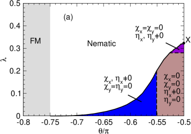
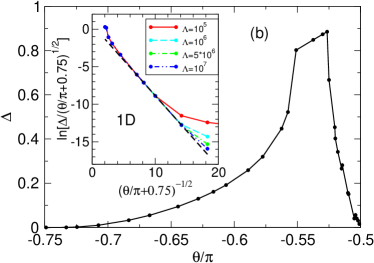
Figure 2: (Color online) (a) Phase diagram of the anisotropic bilinear bi-quadratic spin-1 Heisenberg model in the regime $-0.75\pi\leq\theta\leq-0.5\pi$ ($J\leq K\leq 0$) based on a Schwinger boson mean-field approach. The solid line represents a first-order phase boundary except at $\theta=-0.5\pi$, while the dashed lines represent second-order phase boundaries. The coordinates of the tricritical point X separating the nematic, the Néel ($\theta>-0.5\pi$), and the disordered phases are $\theta_{\text{X}}=-0.5\pi$ and $\lambda_{\text{X}}\approx 0.323$. (b) Energy gap $\Delta$ (in units of 1) along the spin-nematic-disorder phase boundary, which vanishes at $\theta=-0.5\pi$ and $-0.75\pi$. The inset shows the energy gap for a one-dimensional ($\lambda=0$) spin chain of various lengths $\Lambda$ near the critical point at $\theta=-0.75\pi$. A fit to the largest spin chain (black dashed curve) gives $b=\text{ln}(b^{\prime})=-0.945$ and $m=0.945$ (see main text).

For sufficiently large $\lambda$ the ground state is always a spin nematic. However, as one tunes $\lambda$ towards smaller values the nematic gives way to disordered spin liquid phases via a first order transition except at the tricritical points at $\theta=-0.5\pi$ and $-0.75\pi$, where the transition becomes a continuous one. This behavior is corroborated by the energy gap along the phase boundary [Fig. 2(b)]. The gap vanishes as one approaches the points with enlarged SU(3) symmetry at either end of the nematic-disorder phase boundary at $\theta=-0.75\pi$ and $-0.5\pi$. In one dimension [see inset in Fig. 2 (b)], the behavior of the gap near $\theta=-0.75\pi$ can be described by

$$\Delta=b^{\prime}\sqrt{\theta/\pi+0.75}\,\text{exp}\Bigg{(}-\frac{m}{\sqrt{\theta/\pi+0.75}}\Bigg{)},$$ (15)

where $b^{\prime}$ and $m$ are positive constants. It is interesting to note that this form is reminiscent of the Berezinski-Kosterlitz-Thouless-type transition in the (1+1)-dimensional sine-Gordon model. Minnhagen (1987) Equation (15) can be obtained from the constraint equation $\langle\Lambda^{-1}\sum_{k_{x},\alpha}a^{\dagger}_{k_{x},\alpha}a_{k_{x},\alpha}\rangle=N$ by considering the most singular contribution in the $k_{x}=0$ and $\theta=-0.75\pi$ limit and by exploiting the fact that the fields approach a common value $\eta_{x}=\chi_{x}=1/3$ near $\theta=-0.75\pi$. Here, $\Lambda$ denotes the length of the spin chain.

Our results also show no indication of a gapped nematic phase near the ferromagnetic phase in the one-dimensional regime as was proposed by Chubukov. In fact, it is always possible to satisfy the occupancy constraint without a nematic condensate in one dimension. However, at the critical point at $\theta=-0.75\pi$ and $\lambda=0$, the nematic phase merges from the finite $\lambda$ regime, as shown in Fig. 2, so that the nematic correlation function diverges at this point.

Inside the disordered regime we identify three different spin-liquid phases [see Fig. 2(a)]: a one-dimensional Z₂ spin-liquid ($\chi_{x},\eta_{x}\neq 0,\chi_{y}=\eta_{y}=0$), a one-dimensional U(1) spin-liquid ($\eta_{x}\neq 0,\chi_{x}=\chi_{y}=\eta_{y}=0$), and a two-dimensional U(1) spin-liquid ($\eta_{x},\eta_{y}\neq 0,\chi_{x}=\chi_{y}=0$). All three phases are separated from each other by second-order phase boundaries that are located at $\theta_{c}\approx-0.551\pi$ and $\lambda_{c}\approx 0.28$, respectively. The decoupling of the spin chains below $\lambda_{c}$ is likely to be due to the mean-field scheme, which overstates the anisotropy in the quasi-one-dimensional limit. Moreover, due to the one-dimensional nature, we expect only a weak $\lambda$-dependence of the phase boundary between the Z₂ and the one-dimensional U(1) phases, which could not be resolved. The phase boundary between the one-dimensional and the two-dimensional U(1) spin-liquids at $\lambda_{c}$ also does not exhibit any dependence on the $JK$ angle $\theta$. Detailed results along two directions in the phase diagram are shown in Fig. 3.

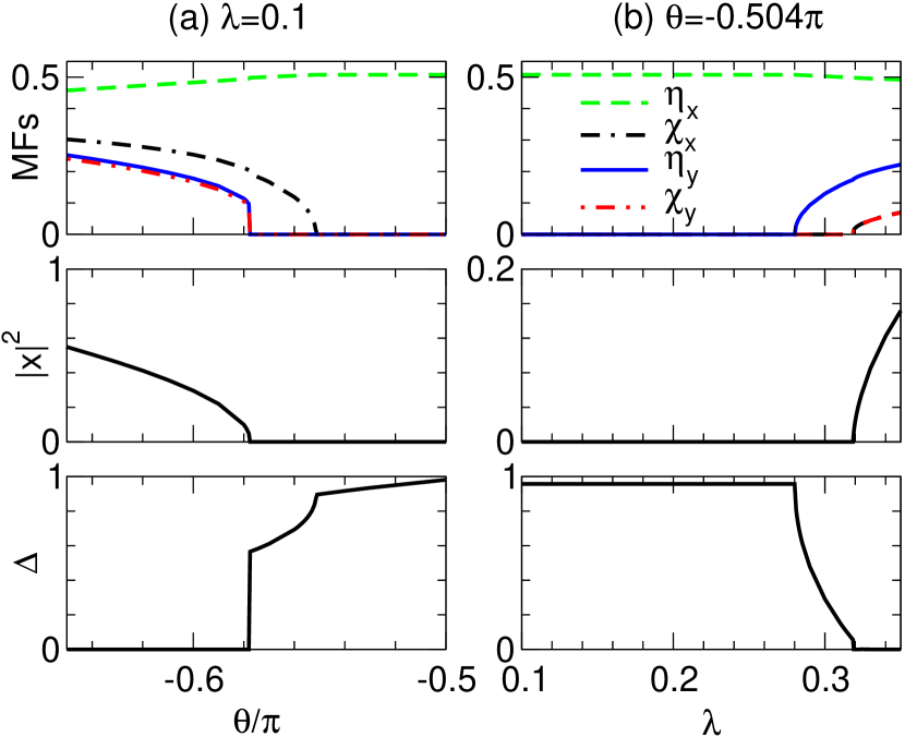
Figure 3: (Color online) Mean field values $\eta_{x},\chi_{x},\eta_{y},\chi_{y}$, “superfluid fraction” $|x|^{2}$, and energy gap $\Delta$ (in units of 1) for cuts (a) parallel and (b) perpendicular to the $\theta$ axis of the phase diagram [Fig.2 (a)].

Last, it is interesting to note that the “unconventional” transition point ($\theta=-0.55\pi$) examined previously in the QMC studies Harada et al. (2007) lies in very close proximity to the Z₂-U(1) phase boundary.

Going beyond mean-field level, saddle-point fluctuations are not likely to change the nature of the first-order phase boundary. We expect on the other hand that Berry phase effects will lead to spontaneous dimerization throughout the $\chi_{y}=\eta_{y}=0$ disordered region, which lies beyond mean-field level. This situation is similar to SU($N$) antiferromagnets, where Berry phase effects arise from nontrivial U(1) gauge-field fluctuations and induce dimer ordering in 1D and 2D. Read and Sachdev (1990, 1989) In particular, following such arguments for the SU(3) ($J=0$) point in the $JK$ model, we expect a columnar dimer ordering for $\lambda<\lambda_{\text{X}}$ [see Fig. 2(a)]. We also expect that the one-dimensional $Z_{2}$ spin-liquid phase with $\chi_{x},\eta_{x}\neq 0$ is unstable towards dimer ordering, which can be understood via a mapping to the odd Ising gauge theory in 1D. Moessner, Sondhi, and Fradkin (2001) Note that a two-dimensional $Z_{2}$ spin liquid phase is absent on mean-field level even at finite $\lambda$. It is possible that small modifications to this model may reveal a two-dimensional $Z_{2}$ spin liquid that, depending on the vison fugacity, may or may not be stable towards dimer ordering. Senthil and Fisher (2000) This is beyond the present study and will be addressed in the near future.

IV Application to optical lattices

Spin systems with a large bi-quadratic contribution are rarely found in solid state systems. However, models with higher-order spin interactions can almost perfectly be realized with ultracold spinor atoms in optical lattices. Moreover, anisotropy-tuned phase transitions between different spin states can easily be induced by changing the optical lattice potential in a particular direction, hence favoring or disfavoring exchange processes between spins along this direction. The spin-nematic-dimer transition also conserves magnetization, which is a fundamental constraint on optical lattice experiments.

Considering the lower $S=1$ hyperfine energy manifold of ²³Na atoms, a large bi-quadratic spin interaction naturally arises in an optical square lattice with a single average occupancy per site. Imambekov et al. (2003); Yip (2003) This follows from the two-dimensional spin-1 Bose-Hubbard model,

$$H_{BH} = -t\sum_{\langle i,j\rangle,\sigma}(b^{\dagger}_{i,\sigma}b_{j,\sigma}+b^{\dagger}_{j,\sigma}b_{i,\sigma})+\frac{U_{0}}{2}\sum_{i}n_{i}(n_{i}-1)$$ (16)

$$+\frac{U_{2}}{2}\sum_{i}({\bf S^{2}_{i}}-2n_{i})-\mu\sum_{i}n_{i},$$

where $b^{\dagger}_{i,\sigma}$ creates a boson on site $i$ with spin $\sigma=0,\pm 1$, $n_{i}=\sum_{\sigma}b^{\dagger}_{i,\sigma}b_{i,\sigma}$ is the number operator, and ${\bf S}_{i}$ denotes the total spin on site $i$. The spin-dependent potential $U_{2}$ originates from the difference in the scattering lengths for the two possible scattering spin channels $S=0$ and $2$ for spin-1 atoms. To leading order in $t/U_{0}$, the effective spin model then results in Eq. (2) (with $\lambda=1$), where the exchange integrals are determined by $J=-2t^{2}/(U_{0}+U_{2})$ and $K=-2t^{2}/(3(U_{0}+U_{2}))-4t^{2}/(3(U_{0}-2U_{2}))$. Typically, for ²³Na atoms one has $U_{2}/U_{0}\approx 0.04$, which translates to $J/K\approx 0.34$, or equivalently, $\theta\approx-0.604\pi$ in the effective spin model. In an anisotropic lattice, the hopping amplitude $t$ becomes directionally dependent, giving rise to anisotropic $J$ and $K$ integrals.

How can one probe the nematic to dimer phase transition? A common way of analyzing optical lattice experiments is to release all atoms from the trap and to measure the column density of the expanding cloud. Within this approach, a straightforward way to observe a spin nematic to dimer phase transition Imambekov et al. (2003) is to apply a weak magnetic field (say along the 3-axis) to align the nematic hard axis perpendicular to the field prior to the release, and to separate different spin components in the expanding cloud spatially by applying a gradient field after the release. A sudden change in the population of the $a^{\dagger}_{3}$ state when tuning $\lambda$ then signals the transition to the dimerized VBS.

Besides this, the interference pattern and the spatial noise correlations of the expanding cloud also provide information about the quantum state in the lattice. Grondalski et al. (1999); Altman et al. (2004); Roth and Burnett (2003); Fölling et al. (2005) For instance, in the case of spin-1 atoms (with mass $m$), the equal-time density-density correlation function for the freely expanding gas after long times takes the form Brennen et al. (2007)

$$G({\bf r},{\bf r}^{\prime}) = \frac{1}{L^{2}}\sum_{\alpha,\beta}\langle n_{\alpha}({\bf r})n_{\beta}({\bf r^{\prime}})\rangle$$

$$\sim -\frac{\text{sin}^{2}\big{(}q_{x}L/2\big{)}\text{sin}^{2}\big{(}q_{y}L/2\big{)}}{L^{2}W^{4}\text{sin}^{2}\big{(}q_{x}/2\big{)}\text{sin}^{2}\big{(}q_{y}/2\big{)}}$$

$$+\frac{1}{L^{2}W^{4}}\sum_{i,j}\text{e}^{i{\bf q}({\bf R}_{i}-{\bf R}_{j})}\langle{\bf S}_{i}{\bf S}_{j}+\big{(}{\bf S}_{i}{\bf S}_{j}\big{)}^{2}\rangle,$$

where ${\bf q}=m({\bf r}-{\bf r^{\prime}})/\hbar t$, $L$ denotes the linear size of the square lattice in units of the lattice parameter, and $W$ is the width of the expanding Wannier states originally centered at lattice sites ${\bf R}_{i}$. Here, we have omitted a delta term from normal ordering and constants of order $1/L^{2}$. The first term stems from the unit occupancy constraint per site, while the second term contains the SU(3) spin structure factor which constitutes the $JK$ model exactly at the nematic-ferromagnetic phase boundary ($J=K<0\Leftrightarrow\theta=-0.75\pi$). The signature of a ferromagnetic condensate therefore is indistinguishable from that of a spin-nematic one. Our interest, however, lies in the nematic-dimer phase transition. To evaluate $G({\bf r},{\bf r}^{\prime})$, we assume complete condensation in the $\alpha$ state $|\phi_{\text{{nem}}}\rangle=\prod_{i}a^{\dagger}_{i,\alpha}|0\rangle$ in the spin nematic phase and obtain $\langle{\bf S}_{i}{\bf S}_{j}+\big{(}{\bf S}_{i}{\bf S}_{j}\big{)}^{2}\rangle_{\text{nem}}=2$ for all $i,j$. In the dimer phase one gets $\langle{\bf S}_{i}{\bf S}_{j}+\big{(}{\bf S}_{i}{\bf S}_{j}\big{)}^{2}\rangle_{\text{dimer}}=2$ if the spins on sites $i$ and $j$ form a singlet and $4/9$ otherwise. The correlation function then takes the form

$$G({\bf r},{\bf r}^{\prime}) \sim -\frac{(1-c)\text{sin}^{2}\big{(}q_{x}L/2\big{)}\text{sin}^{2}\big{(}q_{y}L/2\big{)}}{L^{2}W^{4}\text{sin}^{2}\big{(}q_{x}/2\big{)}\text{sin}^{2}\big{(}q_{y}/2\big{)}}$$ (18)

$$+\frac{2-c}{W^{4}}\big{(}\text{cos}(q_{x})+\text{cos}(q_{y})\big{)}$$

with $c=2$ in the nematic and $4/9$ in the dimer phase. By measuring the density density correlator, both phases can be clearly distinguished as shown in Fig. 4. Assuming a lattice spacing of 532 nm, a time of flight of 20 ms and a detector size of $5\,\mu\text{m}$, the momentum resolution results in $\Delta q/(\pi/a)\approx 0.015$ sufficient to observe the peaks for an $L\approx 100$ lattice ($\text{FWHM}/(\pi/a)\approx 0.02$, where FWHM stands for full width at half maximum).

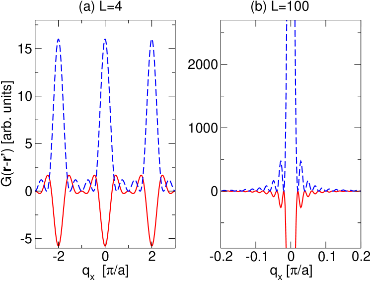
Figure 4: (Color online) Second-order density correlation function for the spin-nematic (blue, dashed curves) and the dimer (red, solid curves) phases for different lattice sizes along the $q_{\text{y}}=0$ direction [${\bf q}=m({\bf r}-{\bf r}^{\prime})/\hbar t$]. The central peak heights are roughly given by $\sim(1-c)L^{2}$ with $c=2$ in the spin nematic and $4/9$ in the dimer phase. Note the different $x$-axis scalings.

Lastly, a recent and interesting proposal for probing the spin configuration in an optical lattice is based on polarization spectroscopy. Eckert et al. (2008, 2008) This kind of measurement leaves the lattice intact as a signature of the spin state is imprinted in the polarization of a probing light beam. By analyzing the noise fluctuations in the polarization of the outgoing light, the dimerized and the spin-nematic phase can be well discriminated.

V Conclusion

In summary, we have considered the spin nematic to dimer phase transition in the anisotropic $JK$ model using a bond operator formalism and a large-$N$ mean field approach. Our analysis generally suggests a first-order spin nematic to dimer transition but would not contradict the possibility of deconfined criticality at $J=0$ ($\theta=-0.5\pi$), where the $JK$ model has an enlarged SU(3) symmetry. Our large-$N$ analysis reveals a critical point at $J=K<0$ ($\theta=-0.75\pi$) where two phase-transition lines, separating the spin-liquid, spin-nematic, and ferromagnetic phases, meet. Although the nematic phase vanishes in 1D, the nematic correlation length diverges at the critical point. We have also argued that the 1D $Z_{2}$ and the 1D and 2D U(1) spin-liquids are unstable toward dimer ordering while the stability of a 2D $Z_{2}$ spin liquid would depend on the vison fugacity. We do not find a 2D $Z_{2}$ spin-liquid at mean-field level but will address a route to such a phase in the future. Finally, we have discussed various ways of observing a spin-nematic to dimer phase transition in optical lattices, where the lattice anisotropy can be tuned through laser intensities. Such experiments eventually provide concrete ways of studying the phases and phase transitions of the $JK$ model.