The puzzling origin of the ⁶Li plateau

Abstract

We discuss the ⁶Li abundance evolution within a hierarchical model of Galaxy formation which correctly reproduces the [Fe/H] distribution of metal-poor halo stars. Contrary to previous findings, we find that neither the level (⁶Li/H$=6\times 10^{-12}$) nor the flatness of the ⁶Li distribution with [Fe/H] can be reproduced under the most favourable conditions by any model in which ⁶Li production is tied to a (data-constrained) Galactic star formation rate via cosmic ray spallation. Thus, the origin of the plateau might be due to some other early mechanism unrelated to star formation.

1 Introduction

The relative abundance of light elements synthesized during the big bang nucleosynthesis (BBN) is a function of a single parameter, $\eta$, namely the baryon-to-photon ratio. Given the WMAP constraint $\eta=(6.8\pm 0.21)\times 10^{-10}$, the light nuclei abundances can be precisely predicted by BBN (Spergel, 2007; Yao & et al., 2006). Despite a general agreement with the observed abundances of light elements, discrepancies arise concerning Li abundance. Observationally, the primordial abundance of lithium isotopes (⁷Li and ⁶Li), is measured in the atmospheres of Galactic metal-poor halo stars (MPHS).

Since the first detection by Spite & Spite (1982), later confirmed by subsequent works (Spite et al., 1984; Ryan et al., 1999; Asplund et al., 2006; Bonifacio, 2007) a ⁷Li/H $=(1-2)\times 10^{-10}$ abundance was deduced, independent of stellar [Fe/H]. The presence of such a ⁷Li plateau supports the idea that ⁷Li is a primary element, synthesized by BBN. The measured value, however, results of a factor $2-4$ lower than the expected from the BBN ⁷Li/H $=4.27^{+1.02}_{-0.83}\times 10^{-10}$ (Cyburt, 2004), ⁷Li/H $=4.9^{+1.4}_{-1.2}\times 10^{-10}$ (Cuoco et al., 2004), or ⁷Li/H $=4.15^{+0.49}_{-0.45}\times 10^{-10}$ (Coc et al., 2004). Recently, Pinsonneault et al. (2002) and Korn et al. (2006) found that mixing and diffusion processes during stellar evolution could reduce the ⁷Li abundance in stellar atmospheres by about 0.2 dex, thus partially releasing the tension.

A more serious problem arose with ⁶Li, for which the BBN predicts a value of (⁶Li/H)${}_{\rm BBN}\sim 10^{-14}$. Owing to the small difference in mass between ⁶Li and ⁷Li, lines from these two isotopes blend easily. The detection of ⁶Li then results quite difficult since the predominance of ⁷Li. Recently, high-resolution spectroscopic observations measured the ⁶Li abundance in 24 MPHS (Asplund et al., 2006), revealing the presence of a plateau ⁶Li/H$=6\times 10^{-12}$ for $-3\lower 1.93748pt\hbox{$\;\buildrel<\over{\sim}\;$}$[Fe/H]$\lower 1.93748pt\hbox{$\;\buildrel<\over{\sim}\;$}-1$. A primordial origin of ⁶Li seems favoured by the presence of the plateau; however, the high ⁶Li value observed cannot be reconciled with this hypothesis.

The solutions invoked to overcome the problem were: (i) a modification of BBN models (Kawasaki et al., 2005; Jedamzik et al., 2006; Pospelov, 2007; Cumberbatch et al., 2007; Kusakabe et al., 2007), (ii) the fusion of ³He accelerated by stellar flares with the atmospheric helium (Tatischeff & Thibaud, 2007), (iii) a mechanism allowing for later production of ⁶Li during Galaxy formation. The latter scenario involves the generation of cosmic rays (CRs). ⁶Li, in fact, can be synthesized by fusion reactions ($\alpha+\alpha\rightarrow\rm\,^{6}Li$) when high-energy CR particles collide with the ambient gas. Energetic CRs can either be accelerated by shock waves produced during cosmological structure formation processes (Miniati et al., 2000; Suzuki & Inoue, 2002; Keshet et al., 2003) or, by strong supernova (SN) shocks along the build-up of the Galaxy. In their recent work Rollinde et al. (2006) used the supernova rate (SNR) by Daigne et al. (2006) to compute the production of ⁶Li in the intergalactic medium (IGM). Assuming that all MPHS form at $z\sim 3$, and from a gas with the same IGM composition, they obtained the observed ⁶Li value. Despite the apparent success of the model, these assumptions are very idealized and require a closer inspection. We revisit the problem using a more realistic and data-constrained approach, based on the recent model by Salvadori et al. (2007) (SSF07), which follows the hierarchical build-up of the Galaxy and reproduces the metallicity distribution of MPHS.

2 Building the Milky Way

The code GAlaxy Merger Tree & Evolution (gamete) described in SSF07 (updated version in Salvadori et al. 2008) follows the star formation (SF)/chemical history of the MW along its merger tree, finally matching all its observed properties.

The code reconstructs the hierarchical merger history of the MW using a Monte Carlo algorithm based on the extended Press & Schechter theory (Press & Schechter, 1974) and adopting a binary scheme with accretion mass (Cole et al., 2000; Volonteri et al., 2003). Looking back in time at any time-step a halo can either lose part of its mass (corresponding to a cumulative fragmentation into haloes below the resolution limit $M_{\rm res}$) or lose mass and fragment into two progenitors. The mass below $M_{\rm res}$ accounts for the Galactic Medium (GM) which represents the mass reservoir into which haloes are embedded. During the evolution, progenitor haloes accrete gas from the GM and virialize out of it. We assume that feedback suppresses SF in mini-haloes and that only Ly$\alpha$ cooling haloes ($T_{\rm vir}>10^{4}$ K) contribute stars and metals to the Galaxy. This motivates the choice of a resolution mass $M_{\rm res}=M_{4}(z)/10=M(T_{\rm vir}=10^{4}$ K $,z)/10$ where $M_{4}(z)$ is the mass corresponding to a virial temperature $T_{\rm vir}=10^{4}$K at redshift $z$. At the highest redshift of the simulation, $z\approx 20$, the gas present in virialized haloes, as in the GM, is assumed to be of primordial composition. The SF rate (SFR) is taken to be proportional to the mass of gas. Following the critical metallicity scenario (Bromm et al., 2001; Schneider et al., 2002, 2003; Omukai et al., 2005; Schneider et al., 2006) we assume that low-mass (Pop II/I) SF occurs when the metallicity $Z_{\rm cr}>10^{-5\pm 1}{Z_{\odot}}$ according to a Larson initial mass function with a characteristic mass $m_{\star}=0.35M_{\odot}$. At lower $Z$ massive Pop III stars form with a characteristic mass $m_{\rm PopIII}=200{M_{\odot}}$, i.e. within the pair-instability supernova (SN_γγ) mass range of $140-260{M_{\odot}}$ (Heger & Woosley, 2002). The chemical evolution of both gas in proto-Galactic haloes (ISM) and in the GM, is computed by according to a mechanical feedback prescription (see Salvadori et al. (2008) for details). Produced metals are instantaneously and homogeneously mixed with the gas.

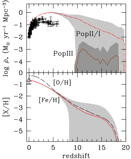
Figure 1: Upper panel: Comoving SFR density evolution for Pop III (solid line) and Pop II/I stars (dashed line). The curves are obtained after averaging over 100 realizations of the merger tree; shaded areas denote $\pm 1\sigma$ dispersion regions around the mean. Points represent the low-redshift measurements of the cosmic SFR by Hopkins (2004). Lower panel: Corresponding GM iron (solid line) and oxygen (dashed line) abundance evolution. The point is the measured [O/H] abundance in high-velocity clouds by Ganguly et al. (2005).

The model free parameters are fixed to match the global properties of the MW and the Metallicity Distribution Function (MDF) of MPHS derived form the Hamburg-ESO Survey (Beers & Christlieb, private communication). In Fig. 1 (upper panel) the derived Galactic (comoving) SFR density is shown for Pop III and Pop II/I stars. Pop II/I stars dominate the SFR at any redshift. Following a burst of Pop III stars, in fact, the metallicity of the host halo raises to $Z>Z_{cr}$: chemical feedback suppresses Pop III formation in self-enriched progenitors. Later on Pop III stars can only form in those haloes which virialize from the GM and so, when $Z_{\mathrm{GM}}\lower 1.93748pt\hbox{$\;\buildrel>\over{\sim}\;$}Z_{cr}$, their formation is totally quenched. The above results are in agreement with recent hydrodynamic simulations implementing chemical feedback effects (Tornatore et al. 2007). The earlier Pop III disappearance of our model ($z\sim 10$) with respect to this study ($z\sim 4$) is a consequence of the biased volume we consider i.e. the MW environment. As the higher mean density accelerates SF/metal enrichment, PopIII stars disappear at earlier times; the SFR maximum value and shape, however, match closely the simulated ones.

In Fig. 1 (lower panel) we show the corresponding evolution of the GM iron and oxygen abundance. As SSF07 have shown that the majority of present-day iron-poor stars ([Fe/H]$<-2.5$) formed in haloes accreting GM gas which was Fe-enhanced by previous SN explosions, the initial [Fe/H] abundance within a halo is set by the corresponding GM Fe-abundance at the virialization redshift.

3 Lithium production

To describe the production of ⁶Li for a continuous source of CRs we generalize the classical work of Montmerle (1977), who developed a formalism to follow the propagation of an homogeneous CR population in an expanding universe, assuming that CRs have been instantaneously produced at some redshift.

Since the primary CRs are assumed to be produced by SNe, the physical source function $Q(E,z)$ is described by a power law in momentum:

$$Q(E,z)=C(z)\frac{\phi(E)}{\beta(E)}\ \mathrm{(GeV/n)}^{-1}\,\mathrm{cm}^{-3}\,\mathrm{s}^{-1}$$ (1)

with $\beta=v/c$ and

$$\phi(E)=\frac{E+E_{0}}{[E(E+2E_{0})]^{(\gamma+1)/2}}\ \mathrm{(GeV/n)}^{-1}\,\mathrm{cm}^{-2}\,\mathrm{s}^{-1}$$ (2)

where $\gamma$ is the injection spectral index and $E_{0}=939$ MeV and $E$ are, respectively, the rest-mass energy and the kinetic energy per nucleon. The functional form of the injection spectrum $\phi(E)$ is inferred from the theory of collisionless shock acceleration (Blandford & Eichler, 1987) and the $\gamma$ value is the one typically associated to the case of strong shock. We note however that the results are only very weakly dependent on the spectral slope. Finally, $C(z)$ is a redshift-dependent normalization; its value is fixed at each redshift by normalizing $Q(E,z)$ to the total kinetic energy transferred to CRs by SN explosions:

$$\mathcal{E}_{\mathrm{SN}}(z)=\int_{E_{\mathrm{min}}}^{E_{\mathrm{max}}}EQ(E,z){\mathrm{d}}E$$ (3)

with

$$\mathcal{E}_{\mathrm{SN}}(z)=\epsilon(1+z)^{3}[E_{{}_{\rm II}}\mathrm{SNR}_{{}_{\rm II}}(z)+E_{\gamma\gamma}\mathrm{SNR}_{\gamma\gamma}(z)]$$ (4)

where $E_{\rm II}=1.2\times 10^{51}$ erg and $E_{\gamma\!\gamma}=2.7\times 10^{52}$ erg are, respectively, the average explosion energies for a Type II SN (SN_II) and a SN${}_{\gamma\!\gamma}$; $\epsilon=0.15$ is the fraction of the total energy not emitted in neutrinos transferred to CRs by a single SN, assumed to be the same for the two stellar populations; SNR_II (SNR${}_{\gamma\!\gamma}$) is the SN_II (SN${}_{\gamma\!\gamma}$) explosion comoving rate, simply proportional to the Pop II/I (Pop III) SFR. The efficiency parameter is inferred by shock acceleration theory and confirmed by recent observations of SN remnants in our Galaxy (Tatischeff, 2008).

We now need to specify the energy limits $E_{\rm min}$, $E_{\rm max}$ of the CR spectrum produced by SN shock waves (eq. 3). We fix $E_{\rm max}=10^{6}$ GeV, following the theoretical estimate by Lagage & Cesarsky (1983). Due to the rapid decrease of $\phi(E)$ the choice of $E_{\rm max}$ does not affect the result of the integration and hence the derived $C(z)$ value. On the contrary $C(z)$ strongly depends on the choice of $E_{\rm min}$: the higher $E_{\rm min}$, the higher is $C(z)$. Since observations cannot set tight constraints on $E_{\rm min}$, due to solar magnetosphere modulation of low-E CRs, we consider it as a free parameter of the model.

Once the spectral shape of $Q(E,z)$ is fixed, we should in principle take in account the subsequent propagation of CRs both in the ISM and GM. Following Rollinde et al. (2006), we make the hypothesis that primary CRs escape from parent galaxies on a timescale short enough to be considered as immediately injected in the GM without energy losses. At high redshift in fact: (i) structures are smaller and less dense (Zhao et al. 2003) implying higher diffusion efficiencies (Jubelgas et al. 2006); (ii) the magnetic field is weaker and so it can hardly confine CRs into structures. Note also that, besides diffusive propagation of CRs, superbubbles and/or galactic winds could directly eject CRs into the GM.

Under this hypothesis the density evolution of primary CRs only depends on energy losses suffered in the GM. The nuclei lose energy mainly via two processes, ionization and Hubble expansion, and they are destroyed by inelastic scattering off GM targets (mainly protons).

We can follow the evolution of $\alpha$-particles (primary CRs) through the transport equation (Montmerle, 1977)

$$\frac{\partial N_{\alpha,\rm H}}{\partial t}+\frac{\partial}{\partial E}(bN_{\alpha,\rm H})+\frac{N_{\alpha,\rm H}}{T_{D}}=K_{\alpha p}Q_{\rm,H}(E,z)$$ (5)

where $N_{i,H}$ is the ratio between the (physical) number density of species $i$ and GM protons, $n_{H}(z)=n_{\rm H,0}(1+z)^{3}$; $Q_{\rm,H}(E,z)\equiv Q(E,z)/n_{\rm H}(z)$ is the normalized physical source function, $b\equiv\left(\partial E/\partial t\right)$ is the total energy loss rate adopted from Rollinde et al. (2006), $T_{D}$ is the destruction term as in the analytic fit by Heinbach & Simon (1995); finally, $K_{\alpha p}=0.08$ is the cosmological abundance by number of $\alpha$-particles with respect to protons.

We consider ⁶Li as entirely secondary, i.e. purely produced by fusion of GM He-nuclei by primary $\alpha$-particles. The physical source function for ⁶Li is given by:

$$Q_{\rm 6Li}(E,z)=\int\sigma_{\alpha\alpha\rightarrow\rm 6Li}(E,E^{\prime})n_{\rm He}(z)\Phi_{\alpha}(E^{\prime},z){\mathrm{d}}E^{\prime}$$ (6)

where $E^{\prime}$ and $E$ are respectively the kinetic energies per nucleon of the incident particle and of the produced ⁶Li nuclei, and $\Phi_{\alpha}(E^{\prime},z)=\beta(E^{\prime})N_{\alpha}(E^{\prime},z)$ the incident $\alpha$-particle flux. Making the approximation $\sigma_{\alpha\alpha\rightarrow\rm 6Li}(E,E^{\prime})=\sigma_{l}(E)\delta(E-E^{\prime}/4)$ (Meneguzzi et al., 1971) and defining $Q_{\rm 6Li,H}\equiv Q_{\rm 6Li}/n_{\rm H}$, the eq. (6) becomes

$$Q_{\rm 6Li,H}(E,z)=\sigma_{l}(E)K_{\alpha p}n_{\rm H}(z)\Phi_{\alpha\rm,H}(4E,z)$$ (7)

where the cross section $\sigma_{l}(E)$ is given by the analytic fit of Mercer (2001):

$$\sigma_{l}(E)\sim 66\exp\left(-\frac{E}{4\ \rm MeV}\right)\ {\rm mb}$$ (8)

We can now write a very simple equation describing the evolution of ⁶Li:

$$\frac{\partial N_{\rm 6Li,H}}{\partial t}=Q_{\rm 6Li,H}(E,z)$$ (9)

in this case, in fact, destruction and energy losses are negligible since their time scales are very long with respect to the production time scale (Rollinde et al., 2005).

The solution of the coupled eqs. (5)-(9) gives ⁶Li/H at any given redshift $z$.

4 Results

The system of equations introduced in the previous Sec. are solved numerically using a Crank-Nicholson implicit numerical scheme (Press, 2002). Because of its stability and robustness implicit schemes are used to solve transport equations in most CRs diffusion problems (Strong & Moskalenko, 1998).

We test the accuracy of our code by studying a simplified case in which an analytic solution can be derived and compared with numerical results. To this aim we assume that: (i) both energy losses and destruction of primary CRs in the GM can be neglected; (ii) the physical energy density injected by SNe is constant, ${\cal E}_{\rm SN}\sim 7.4\times 10^{-27}$ GeV cm^-3 s^-1, in the redshift range $z>3$. It is worth noting that the above hypothesis conspire to give an upper limit to the exact solution, thus providing an estimate of the maximum achievable ⁶Li abundance. Under these approximations, the source spectrum defined in eq. (1) becomes:

$$Q(E,z)=\rm 6.4\cdot 10^{-29}\frac{\phi(E)}{\beta(E)}\ \mathrm{(GeV/n)}^{-1}\,\mathrm{cm}^{-3}\,\mathrm{s}^{-1}$$ (10)

and eqs. (5)-(9) can be solved. We find

$$N_{\alpha,\rm H}(z)=39.6\,(1+z)^{-9/2}$$ (11)

and

$$N_{\rm 6Li,H}(z)=8.2\times 10^{-11}(1+z)^{-3}$$ (12)

From Fig. 2 we conclude that the analytical solution for the GM ⁶Li abundance (eq. 12) is perfectly matched by the numerical one. Also shown are the numerical solutions obtained by relaxing first the hypothesis (i) and then (i) + (ii). Not unexpectedly, the inclusion of energy losses and destruction term into eq. (5) affects only slightly the result, as the typical time-scales of such processes are longer than the ⁶Li production one.

A realistic injection energy, on the contrary, has a strong impact on the predicted shape and amplitude of the ⁶Li evolution. In fact, the SFR, and consequently ${\cal E}_{\rm SN}$, is an increasing function of time in the analyzed redshift range (Fig. 1 upper panel). The maximum ${\cal E}_{\rm SN}$ we can obtain by using the SNR derived from the curve in Fig. 1, a realistic energy transfer efficiency $\epsilon=0.15$, and $E_{\rm min}=10^{-5}$ GeV (Rollinde et al., 2006), is ${\cal E}_{\rm SN}^{max}\sim 8.6\times 10^{-28}<7.4\times 10^{-27}$ GeV cm^-3 s^-1. Note that the ⁶Li/H abundance at $z=3$ results more than 1 order of magnitude smaller than the value of the simplified case. In the following, we will refer to this physical model as our fiducial model.

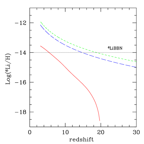
Figure 2: Redshift evolution of GM ⁶Li/H abundance for the analytical (green short-dashed line) and numerical solution (overlapped) of a simplified model with no energy losses and destruction, and ${\cal E}_{\rm SN}=7.4\times 10^{-27}$ GeV cm^-3 s^-1 for $z>3$, the same model including energy loss/destruction (blue long dashed line), the fiducial model with realistic SNR, $\epsilon=0.15$ and $E_{\rm min}=10^{-5}$ MeV (red solid line).

We now use the [Fe/H] predicted by GAMETE (Fig. 1, lower panel) to convert redshift into [Fe/H] values and derive the GM ⁶Li vs [Fe/H]. According to our semi-analytical model for the build-up of the MW, in fact, the GM elemental abundances reflect those of MPHS, which are predicted to form out of new virializing haloes accreting gas from the GM. This implies that the observed MPHS formed continuously within the redshift range $3<z\leq 10$. From Fig. 3 we see that our fiducial model yields log ⁶Li/H$=-13.5$, i.e. about three orders of magnitude below the data.

This discrepancy cannot be cured by simply boosting the free parameters to their maximum allowed values. This is also illustrated in the same Figure, where for the upper curve we assume $\epsilon=1$, $E_{\rm min}=10$ MeV/n and for the SFR the maximum value allowed by GAMETE within 1-$\sigma$ dispersion. Although the discrepancy between observations and model results is less prominent in this case, we are still unable to fit the data, in particular at [Fe/H] $=-3$ (i.e. at higher redshifts) only Log ⁶Li/H$=-12.6$ has had time to be produced, failing short by $30$ times.

In addition the flat data distribution cannot be recovered. It is worth noting that, as also pointed out by Asplund et al. (2006) ⁶Li may be depleted in stars, mainly during the pre-main sequence phase. If this is the case, the ⁶Li abundance observed in stars would not be representative of the gas from which they have formed. Taking into account this effect the inferred ⁶Li abundances become metallicity dependent, i.e. the flatness is lost. Because of depletion however, the derived ⁶Li values would be higher for all [Fe/H], making the discrepancy between our results and observations even larger.

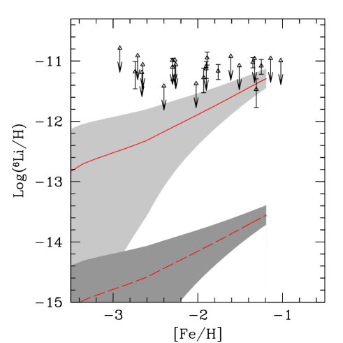
Figure 3: Redshift evolution of ⁶Li/H vs [Fe/H] for the fiducial model ($\epsilon=0.15$, $E_{\rm min}=10^{-5}$ GeV/n, dashed line) and for the maximal model ($\epsilon=1$, $E_{\rm min}=10$ MeV/n, solid line). Shaded areas denote $\pm 1\sigma$ dispersion regions around the mean.

We finally note, as already claimed by Rollinde et al. (2006), that the production of ⁷Li through this mechanism is comparable with that of ⁶Li , being the production cross sections of the two isotopes very similar. No overproduction of ⁷Li is then expected with respect of the BBN-based value.

5 Discussion

We have pointed out that both the level and flatness of the ⁶Li distribution cannot be explained by CR spallation if these particles have been accelerated by SN shocks inside MW building blocks. Although previous claims (Rollinde et al., 2006) of a possible solution invoking the production of ⁶Li in an early burst of PopIII stars have been put forward, such scenario is at odd with both the global properties of the MW and its halo MPHS.

Our model, which follows in detail the hierarchical build-up of the MW and reproduces correctly the MDF of the MPHS, predicts a monotonic increase of ⁶Li abundance with time, and hence with [Fe/H]. Moreover, our fiducial model falls short of three orders of magnitude in explaining the data; such discrepancy cannot be cured by allowing the free parameters ($E_{\rm min},\epsilon$) to take their maximum (physically unlikely) values. Apparently, a flat ⁶Li distribution appears inconsistent with any (realistic) model for which CR acceleration energy is tapped from SNe: if so, ⁶Li is continuously produced and destruction mechanisms are too inefficient to prevent its abundance to steadily increase along with [Fe/H].

Clearly, the actual picture could be more complex: for example, if the diffusion coefficient in the ISM of the progenitor galaxies is small enough, ⁶Li could be produced in situ rather than in the more rarefied GM. This process might increase the species abundance, but cannot achieve the required decoupling of ⁶Li evolution from the enrichment history.

Alternatively, shocks associated with structure formation might provide an alternative ⁶Li production channel (Suzuki & Inoue, 2002); although potentially interesting as this mechanisms decouples metal enrichment (governed by SNe) and CR acceleration (due to structure formation shocks), the difficulties that this scenario must face are that (i) at the redshifts ($z=2-3$) at which shocks are most efficient it must be still [Fe/H]$<-3$, and (ii) MPHS that formed at earlier epochs should have vanishing ⁶Li abundance (Prantzos, 2006).

If these issues could represent insurmountable problems, then one has to resort to more exotic models involving either suitable modifications of BBN or some yet unknown production mechanism unrelated to cosmic SF history.

References

- Asplund et al. (2006) Asplund M., Lambert D. L., Nissen P. E., Primas F., Smith V. V., 2006, ApJ, 644, 229
- Blandford & Eichler (1987) Blandford R., Eichler D., 1987, Phys. Rep., 154, 1
- Bonifacio (2007) Bonifacio P. e. a., 2007, A&A, 462, 851
- Bromm et al. (2001) Bromm V., Ferrara A., Coppi P. S., Larson R. B., 2001, MNRAS, 328, 969
- Coc et al. (2004) Coc A., Vangioni-Flam E., Descouvemont P., Adahchour A., Angulo C., 2004, ApJ, 600, 544
- Cole et al. (2000) Cole S., Lacey C. G., Baugh C. M., Frenk C. S., 2000, MNRAS, 319, 168
- Cumberbatch et al. (2007) Cumberbatch D., et al., 2007, Phys. Rev., D76, 123005
- Cuoco et al. (2004) Cuoco A., Iocco F., Mangano G., Miele G., Pisanti O., Serpico P. D., 2004, International Journal of Modern Physics A, 19, 4431
- Cyburt (2004) Cyburt R. H., 2004, Phys. Rev. D, 70, 023505
- Daigne et al. (2006) Daigne F., Olive K. A., Silk J., Stoehr F., Vangioni E., 2006, ApJ, 647, 773
- Ganguly et al. (2005) Ganguly R., Sembach K. R., Tripp T. M., Savage B. D., 2005, ApJS, 157, 251
- Heger & Woosley (2002) Heger A., Woosley S. E., 2002, ApJ, 567, 532
- Heinbach & Simon (1995) Heinbach U., Simon M., 1995, ApJ, 441, 209
- Hopkins (2004) Hopkins A. M., 2004, ApJ, 615, 209
- Jedamzik et al. (2006) Jedamzik K., Choi K.-Y., Roszkowski L., Ruiz de Austri R., 2006, JCAP, 7, 7
- Kawasaki et al. (2005) Kawasaki M., Kohri K., Moroi T., 2005, Phys. Rev. D, 71, 083502
- Keshet et al. (2003) Keshet U., Waxman E., Loeb A., Springel V., Hernquist L., 2003, ApJ, 585, 128
- Korn et al. (2006) Korn A. J., Grundahl F., Richard O., Barklem P. S., Mashonkina L., Collet R., Piskunov N., Gustafsson B., 2006, Nat, 442, 657
- Kusakabe et al. (2007) Kusakabe M., Kajino T., Boyd R. N., Yoshida T., Mathews G. J., 2007, Phys. Rev. D, 76, 121302
- Lagage & Cesarsky (1983) Lagage P. O., Cesarsky C. J., 1983, A&A, 125, 249
- Meneguzzi et al. (1971) Meneguzzi M., Audouze J., Reeves H., 1971, A&A, 15, 337
- Mercer (2001) Mercer D. J. e. a., 2001, Phys. Rev. C, 63, 065805
- Miniati et al. (2000) Miniati F., Ryu D., Kang H., Jones T. W., Cen R., Ostriker J. P., 2000, ApJ, 542, 608
- Montmerle (1977) Montmerle T., 1977, ApJ, 216, 177
- Omukai et al. (2005) Omukai K., Tsuribe T., Schneider R., Ferrara A., 2005, ApJ, 626, 627
- Pinsonneault et al. (2002) Pinsonneault M. H., Steigman G., Walker T. P., Narayanan V. K., 2002, ApJ, 574, 398
- Pospelov (2007) Pospelov M., 2007, Phys. Rev. Lett., 98, 231301
- Prantzos (2006) Prantzos N., 2006, A&A, 448, 665
- Press (2002) Press W. H., 2002, Numerical recipes in C++ : the art of scientific computing. Numerical recipes in C++ : the art of scientific computing by William H. Press. xxviii, 1,002 p. : ill. ; 26 cm. Includes bibliographical references and index. ISBN : 0521750334
- Press & Schechter (1974) Press W. H., Schechter P., 1974, ApJ, 187, 425
- Rollinde et al. (2005) Rollinde E., Vangioni E., Olive K., 2005, ApJ, 627, 666
- Rollinde et al. (2006) Rollinde E., Vangioni E., Olive K. A., 2006, ApJ, 651, 658
- Ryan et al. (1999) Ryan S. G., Norris J. E., Beers T. C., 1999, ApJ, 523, 654
- Salvadori et al. (2008) Salvadori S., Ferrara A., Schneider R., 2008, MNRAS, 386, 348
- Salvadori et al. (2007) Salvadori S., Schneider R., Ferrara A., 2007, MNRAS, 381, 647
- Schneider et al. (2002) Schneider R., Ferrara A., Natrajan P., Omukai K., 2002, ApJ, 571, 30
- Schneider et al. (2003) Schneider R., Ferrara A., Salvaterra R., Omukai K., Bromm V., 2003, Nat, 422, 869
- Schneider et al. (2006) Schneider R., Omukai K., Inoue A. K., Ferrara A., 2006, MNRAS, 369, 1437
- Spergel (2007) Spergel D. N. et al.., 2007, ApJS, 170, 377
- Spite & Spite (1982) Spite F., Spite M., 1982, A&A, 115, 357
- Spite et al. (1984) Spite M., Spite F., Maillard J. P., 1984, A&A, 141, 56
- Strong & Moskalenko (1998) Strong A. W., Moskalenko I. V., 1998, ApJ, 509, 212
- Suzuki & Inoue (2002) Suzuki T. K., Inoue S., 2002, ApJ, 573, 168
- Tatischeff (2008) Tatischeff V., 2008, ArXiv e-prints, 804
- Tatischeff & Thibaud (2007) Tatischeff V., Thibaud J.-P., 2007, A&A, 469, 265
- Tornatore et al. (2007) Tornatore L., Ferrara A., Schneider R., 2007, MNRAS, 382, 945
- Volonteri et al. (2003) Volonteri M., Haardt F., Madau P., 2003, ApJ, 582, 559
- Yao & et al. (2006) Yao W.-M., et al. 2006, Journal of Physics G Nuclear Physics, 33, 1