Spectral luminosity indicators in SNe Ia -
Understanding the $\mathcal{R}$(Si ii) line strength ratio and beyond.

Abstract

SNe Ia are good distance indicators because the shape of their light curves, which can be measured independently of distance, varies smoothly with luminosity. This suggests that SNe Ia are a single family of events. Similar correlations are observed between luminosity and spectral properties. In particular, the ratio of the strengths of the Si ii $\lambda 5972$ and $\lambda 6355$ lines, known as $\mathcal{R}$(Si ii), was suggested as a potential luminosity indicator. Here, the physical reasons for the observed correlation are investigated. A Monte-Carlo code is used to construct a sequence of synthetic spectra resembling those of SNe with different luminosities near $B$ maximum. The influence of abundances and of ionisation and excitation conditions on the synthetic spectral features is investigated. The ratio $\mathcal{R}$(Si ii) depends essentially on the strength of Si ii $\lambda 5972$, because Si ii $\lambda 6355$ is saturated. In less luminous objects, Si ii $\lambda 5972$ is stronger because of a rapidly increasing Si ii/Si iii ratio. Thus, the correlation between $\mathcal{R}$(Si ii) and luminosity is the effect of ionisation balance. The Si ii $\lambda 5972$ line itself may be the best spectroscopic luminosity indicator for SNe Ia, but all indicators discussed show scatter which may be related to abundance distributions.

1 Introduction

Type Ia supernovae (SNe Ia) form a relatively homogeneous supernova subclass. They supposedly originate from accreting C-O white dwarfs that undergo explosive burning as they approach the Chandrasekhar mass limit (Hillebrandt & Niemeyer, 2000). Their enormous light output is powered by radioactivity of synthesised ⁵⁶Ni and of its daughter nuclide ⁵⁶Co (Arnett, 1982).

Differences in the synthesised ⁵⁶Ni mass result in a spread in luminosity of $\sim\!\!3$ mag in the $B$ band (Mazzali et al., 2001, 2007). Phillips (1993) found that the decline in $B$-band magnitude within 15 days after $B$ maximum, $\Delta m_{15}(B)$, correlates inversely with the $B$-band maximum luminosity $M_{B,\textrm{max}}$ and thus can be used as a luminosity indicator. Thus, SNe Ia can be used as distance indicators in cosmological studies (“standard candles”).

Optical spectra reflect in detail the variations among SNe Ia. In the photospheric phase, which lasts until a few weeks after maximum light, P-Cygni features (blueshifted absorption plus less prominent emission centred at the rest wavelength) are superimposed on a “pseudo-continuum” (Pauldrach et al., 1996). The line positions and strengths depend on the abundances and on the excitation and ionisation conditions within the debris. Nugent et al. (1995) showed that the ratio of the depths of two Si ii lines ($\lambda 5972$ and $\lambda 6355$) at $B$-band maximum, $\mathcal{R}$(Si ii), is larger for dimmer SNe, and suggested that this is due to temperature differences. Accordingly, $\mathcal{R}$(Si ii) could be used as a distance-independent spectroscopic luminosity indicator (e.g. Bongard et al., 2006). Other spectral features have subsequently been suggested as possible luminosity indicators (Hachinger, Mazzali & Benetti 2006, hereafter Paper I; Bongard et al. 2006; Foley, Filippenko & Jha 2008). Still, the detailed physics behind the $\cal R$(Si ii)-$L$ correlation have not been explained.

This is the purpose of this work, where we explain the $\cal R$(Si ii)-$L$ correlation investigating the details of the connection between the physics of the envelope and line strengths. We present a sequence of spectral models calculated with a Monte-Carlo (MC) radiative transfer code. The synthetic spectra resemble real SNe with different luminosities shortly after $B$ max. In the model atmospheres, we analyse the conditions which influence the line strengths entering $\cal R$(Si ii).

In the following, first we describe the concept of the synthetic spectral sequence (Sec. 2). In Sec. 3, we show that our models reproduce the $\cal R$(Si ii)-$L$ correlation. In Sec. 4 we explain the correlation analysing the details of the formation of the lines contributing. After discussing spectral luminosity indicators and other applications of line-strength measurements (Sec. 5), we give conclusions (Sec. 6).

2 Concept of the model sequence

2.1 Model SN envelope and radiative transfer simulation

Our work makes use of a 1D Monte Carlo (MC) radiative transfer code (Abbott & Lucy 1985, Mazzali & Lucy 1993, Lucy 1999 and Mazzali 2000, which describes the version used in this work) to compute synthetic SN spectra. The code has successfully been applied to many SNe (SN 1990N: Mazzali et al. 1993, etc.).

The code computes the radiative transfer through the SN above an assumed photosphere. The envelope is assumed to expand homologously (e.g. Röpke & Hillebrandt 2005), meaning that the ejecta move radially with $r=v\cdot t$, where $r$ is the distance from the centre, $t$ the time from explosion and $v$ the velocity. Radius and velocity can therefore be used interchangeably for each gas particle. The density structure is taken from a standard explosion model (W7, Nomoto, Thielemann & Yokoi 1984), scaled according to the time $t$. The chemical composition of the model atmosphere can be freely adjusted, but is assumed to be homogeneous in radius.

From the photosphere, which is located at an adjustable $v_{\textrm{ph}}$, “packets” of thermal radiation [$I_{\nu}^{+}=B_{\nu}(T_{\textrm{ph}})$] are emitted into the atmosphere. As they propagate through the atmosphere, radiation packets can undergo Thomson scattering on electrons or line excitation-deexcitation processes, which are treated in the Sobolev approximation. The process of photon branching is included, which implies that the transitions for excitation and deexcitation can be different. In all processes, radiative equilibrium is conserved. Taking the backscattering into account, the code matches a given output luminosity $L$.

The action of the radiation field onto the gas is calculated using a modified nebular approximation, which mimics the effects of NLTE. The envelope is discretised into 80 shells. For each shell, a radiation temperature $T_{R}$ and a dilution factor $W$ are calculated. These quantities mostly determine the excitation and ionisation state.

The code iterates the radiation field and the gas conditions. After convergence, the output spectrum is obtained from a formal integral solution of the transfer equation (Lucy, 1999).

2.2 Sequence of synthetic spectra

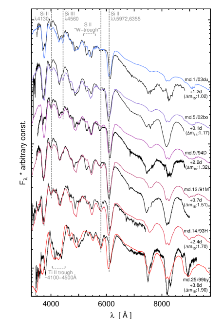
Figure 1: Selected spectra from the model sequence, and observed counterparts (black) with $\Delta m_{15}(B)$ values (see Paper I). All spectra are plotted logarithmically and have been adapted to the total reddening of SN 2003du. Approximate identifications are given for features relevant for this work.

For our study we computed a sequence of 25 spectral models. The start and end points of the sequence were chosen to match a luminous SN Ia (model no. 1: SN 2003du, $\Delta m_{15}(B)$$=1.02$, $M_{B\textrm{,model}}=-19.16$) and a dim one (model no. 25: SN 1999by, $\Delta m_{15}(B)$$=1.90$, $M_{B\textrm{,model}}=-16.86$), respectively, close to $B$ maximum. Observed and synthetic spectra are shown in Fig. 1; further data and references are given in Table 1.

The free model parameters shown in Table 2 and Fig. 2 were iterated to optimise the fit. Some deviations between models and data remain, but they have no influence on our investigation. In the luminous models there is an excess flux in the red caused by the assumption of a blackbody lower boundary. Dim models show a mismatch in line velocities, which should vanish with a refined density and abundance stratification (cf. Taubenberger et al. 2008).

Table 1: First (no. 1) and last (no. 25) model of the sequence: Data of the objects and spectra used for modelling.

Object/epoch/	$\!\!\!\!\Delta m_{15}\!\!\!\!$	Total reddening	Distance modulus	Redshift	References
model no.	[mag]	$\!\!\!\!\!\!E(B-V)^{\textrm{a)}}$ [mag]	$\mu$ [mag]	$z$	for SN,$\mu$,$z$
03du/+1.2d/#1	1.02	0.01	32.79	0.0068	Stanishev et al. (2007)
99by/+3.9d/#25	1.90	0.01	30.75	0.0021	Garnavich et al. (2004)${}^{\textrm{b)}}\!\!\!\!$

${}^{\textrm{a)}}$ The values given represent the galactic extinction $E(B-V)_{\textrm{gal}}$, as the host galaxy extinction is approximately zero for both SNe (see references). $E(B-V)_{\textrm{gal}}$: from NED (see acknowledgements); we averaged the Burstein & Heiles (1982) and Schlegel, Finkbeiner & Davis (1998) values.
${}^{\textrm{b)}}$ Spectrum combined from original spectra with different grating setups (taken between JD 2451312.64 and 2451312.66, available at http://www.cfa.harvard.edu/supernova/) and fine-calibrated to match photometry by multiplying with a linear function (using IRAF and SYNPHOT routines/data, see acknowledgements).

Table 2: Overview of the final parameters for models no. 1 and 25. Mass fractions less significant have been omitted.

Model	$\lg\left(\frac{L}{L_{\odot}}\right)$	$v_{\textrm{ph}}$	$t^{a}$	Element abundances (mass fractions)
		[km s-1]	[d]	$X$(O)	$X$(Mg)	$X$(Si)	$X$(S)	$X$(Ca)	$X$(Ti)	$X$(Cr)	$X$(Fe)${}_{0}{}^{\textrm{b)}}$	$X$(56Ni)${}_{0}{}^{\textrm{b)}}$
no.  1: 03du/+1.2	9.61	8900	21.0	0.056	0.13	0.56	0.19	0.0075	0.0006	0.0006	0.0075	0.060
no. 25: 99by/+3.8	8.82	6500	21.0	0.68	0.085	0.21	0.016	0.0008	0.0016	0.0016	0.0002	0.0025

${}^{\textrm{a)}}$ Time from explosion onset. The rise times for 03du and 99by are assumed to be 19.8d and 17.1d, respectively. This complies with observational studies (Riess et al., 1999; Conley et al., 2006) and leads to a similar time from explosion of $\sim\!\!21.0$d for both models.
${}^{\textrm{b)}}$ The abundances of Fe, Co and Ni in our models are assumed to be the sum of ⁵⁶Ni and its decay chain products (⁵⁶Co and ⁵⁶Fe) on the one hand, and directly synthesised / progenitor Fe on the other hand. Thus, they are conveniently given in terms of the ⁵⁶Ni mass fraction at $t=0$ [$X($⁵⁶Ni$)_{0}$], the Fe abundance at $t=0$ [$X(\textrm{Fe})_{0}$], and the time from explosion onset $t$.

The focus of our fits is on obtaining a reasonable temperature structure. The decrease of temperature from luminous to dim SNe not only implies that the spectra appear redder, but also influences line strengths and $\cal R$(Si ii) via excitation and ionisation. Choosing appropriate models for SNe 03du and 99by as the ends of the sequence, we ensure that we explore a realistic range of temperatures. The temperature structure of our models can to some degree be influenced by the choice of photospheric velocity. We fitted the pseudo-continuum of both SNe as well as possible. We did not increase temperatures further for SN 03du, because this would make Si iii $\lambda 4560$ too strong. The resulting effective temperatures (cf. Nugent et al. 1995)

$$T_{\textrm{eff}}=\frac{L^{1/4}}{(4\pi\sigma_{B})^{1/4}(v_{\textrm{ph}}\cdot t)^{1/2}}$$

($\sigma_{B}$: Stefan-Boltzmann’s constant; $t\approx 21.0\textrm{d}$: time from explosion) of our models are shown in Fig. 3. For comparison we also give the photospheric temperatures $T_{\textrm{ph}}$ which are calculated by the code, taking the backscattering into account.

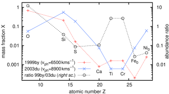
Figure 2: Abundances of the 99by and 03 du model. The Fe and Ni abundances given are $X$(Fe)₀ and $X$(⁵⁶Ni)₀ (see tab. 2). The SN 99by model is generally characterised by very small abundances of burning products, except for relatively large amounts of Ti and Cr (Fig. 2). Despite the decrease in Si abundance, Si ii $\lambda 5972$ is stronger in dimmer objects.

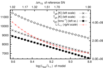
Figure 3: Input parameters $L_{\textrm{bol}}$ and $v_{\textrm{ph}}$ of our models, and resulting effective temperature $T_{\textrm{eff}}$. The photospheric blackbody temperature $T_{\textrm{ph}}$ after convergence is given for comparison.

The other models of the sequence (no. 2-24) were calculated decreasing $\log L$ in constant steps. This leads to a relatively uniform distribution of models in $M_{B}$. The photospheric velocity and all element abundances were changed by constant amounts from one model to the next. An exception is the sulphur abundance: in order to match the evolution of the S ii “W-trough” better, it decreases with a larger slope among luminous SNe and with a smaller slope among dim ones.

We assign $\Delta m_{15}(B)$ values to the models no. 1 and 25 and to four intermediate ones. In order crudely to assign $\Delta m_{15}(B)$ values to intermediate models, we created “optimal-fit” models of the SNe 2002bo [$\Delta m_{15}(B)$$=1.17$], 1994D [$\Delta m_{15}(B)$$=1.32$], 1991M [$\Delta m_{15}(B)$$=1.51$] and 1993H [$\Delta m_{15}(B)$$=1.70$] as reference models. We then compared the sequence models to these by calculating a weighted sum of quadratic deviations in the input parameters ($L_{\textrm{bol}}$, $v_{\textrm{ph}}$ and abundances), where the deviation in $L_{\textrm{bol}}$ was given the strongest weight. The $\Delta m_{15}(B)$ values of the reference models were then assigned to the four sequence models that gave the closest match.

Fig. 1 shows the spectral models assigned a $\Delta m_{15}(B)$ value with their observed counterparts (SN 2002bo: Benetti et al. 2004, SN 1994D: Patat et al. 1996, SN 1991M: Asiago archive, SN 1993H: CTIO archive, with kind permission of M. M. Phillips).

3 R(Si II) in the model sequence

3.1 Line-strength measurements

In order to compare models and observations, we measured the strengths of Si ii $\lambda 5972$ and Si ii $\lambda 6355$, and $\mathcal{R}$(Si ii) in synthetic and observed spectra.

To quantify the line strength, the flux level inside a feature is compared to an estimated “pseudo-continuum”, which we define as a linear function approximately tangential to the spectrum at the edges of the feature. We then measure the line strength as fractional depth:

$$F\>\!\!D(\lambda_{F\>\!\!D}):=\frac{F_{PC}(\lambda_{F\>\!\!D})-F(\lambda_{F\>\!\!D})}{F_{PC}(\lambda_{F\>\!\!D})}\textrm{,}$$ (1)

where $F(\lambda_{F\>\!\!D})$ and $F_{PC}(\lambda_{F\>\!\!D})$ are the actual flux and the pseudo-continuum, respectively, at a wavelength $\lambda_{F\>\!\!D}$, which is chosen so as to obtain the maximum FD. To avoid the influence of noise, measurements were made in spectra convolved with a normalised Gaussian function (FWHM: 15Å).

3.2 Evolution of FDs and $\mathcal{R}$(Si ii)

Fig. 4 shows our measurements of $\textrm{{ FD}}(\textrm{Si\leavevmode\nobreak\ {\sc ii}\ }\lambda 5972)$ and $\textrm{{ FD}}(\textrm{Si\leavevmode\nobreak\ {\sc ii}\ }\lambda 6355)$. While $\textrm{{ FD}}(\textrm{Si\leavevmode\nobreak\ {\sc ii}\ }\lambda 5972)$ clearly increases with decreasing luminosity, $\textrm{{ FD}}(\textrm{Si\leavevmode\nobreak\ {\sc ii}\ }\lambda 6355)$ is approximately constant in all measurements. The resulting ratio $\textrm{{ FD}}(\textrm{Si\leavevmode\nobreak\ {\sc ii}\ }\lambda 5972)/\textrm{{ FD}}(\textrm{Si\leavevmode\nobreak\ {\sc ii}\ }\lambda 6355)\!\sim\!\mathcal{R}(\textrm{Si\leavevmode\nobreak\ {\sc ii}})$ is shown in Fig. 5. The value increases towards lower luminosities.

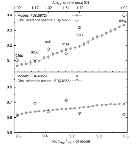
Figure 4: $\lambda 5972$ and $\lambda 6355$ FD in models and observed reference spectra.

Observed spectra are less well behaved than the synthetic ones, and show some constant deviation at the dim end. This could be improved with more sophisticated models using abundance stratification (e.g. Stehle et al., 2005), possibly including some contribution of Na i D to the $\lambda 5972$ feature in dim SNe [See e.g. Filippenko et al. (1992). Na i would make too broad a contribution to the $\lambda 5972$ feature in our homogeneous models.]. Yet, the qualitative evolution of the two Si ii features, as well as their different behaviour, is correctly reproduced.

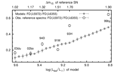
Figure 5: Ratio of Si ii $\lambda 5972$ to Si ii $\lambda 6355$ FD [$\sim\!\!\mathcal{R}$(Si ii)].

4 Analysis

Here we analyse the behaviour of $\mathcal{R}$(Si ii), which is rooted in the evolution of Si ii $\lambda 5972$ and Si ii $\lambda 6355$. We show that the latter line is easily saturated because it is very strong. Si ii $\lambda 5972$, in contrast, is stronger in dimmer objects owing to a larger fraction of Si ii.

Furthermore, we investigate if Ti ii lines have an influence on $\mathcal{R}$(Si ii), as proposed by Garnavich et al. (2004).

4.1 Quantifying the conditions for absorption in our models

Absorption strengths are determined by intrinsic line strengths, abundances, density, ionisation and excitation structure. For absorptions which are (mostly) caused by a single ion, line formation can be conveniently analysed. Before performing the analysis, we introduce our method and quantities important in this context.

Region of the envelope relevant for absorption at $\lambda_{F\>\!\!D}$

The reference wavelength of a FD, $\lambda_{F\>\!\!D}$, is blueshifted with respect to the rest frame wavelength $\lambda_{\textrm{rest}}$, because absorption occurs in material moving towards the observer. Therefore, as seen from the observer’s point of view, the processes relevant for a particular FD take place within a thin layer where the atoms have a line-of-sight (ray-parallel) velocity $v_{||}=(1-\frac{\lambda_{F\>\!\!D}}{\lambda_{\textrm{rest}}})\cdot c$. In the narrow-line limit (Sobolev approximation), with $\boldsymbol{v}\propto\boldsymbol{r}$, this zone is an infinitely thin “iso-$v_{||}$ plane” perpendicular to the ray.

The code calculates physical quantities describing absorption in each radial shell. Thus, a weighted average over several shells is required to obtain values corresponding to a measured FD (and the respective iso-$v_{||}$ plane). This is denoted by angle brackets “$<...>$” below. The weight of each shell is determined by the number of photons impinging on the absorption surfaces of the multiplet within the shell.

Sobolev optical depth and absorption fraction

Both of the features in $\mathcal{R}$(Si ii) are doublets ($\lambda\lambda 5958,5979$ and $\lambda\lambda 6347,6371$, respectively). The total fraction of photons absorbed (“absorption fraction” $\mathfrak{A}$), which is expected to correspond to FD values, can then be calculated as:

$$\mathfrak{A}:=\langle 1-\prod_{l}e^{-\tau_{l,k}}\rangle,$$ (2)

where $\tau_{\textrm{l,k}}$ is the Sobolev optical depth for line $l$ in shell $k$, defined as

$$\tau_{l,k}=t\cdot\frac{hc}{4\pi}n_{i}\big{|}_{k}B_{ij}\left(1-\frac{g_{i}n_{j}}{g_{j}n_{i}}\Big{|}_{k}\right).$$ (3)

Here, $n_{i}$ and $n_{j}$ are the number density of ions in the lower and upper level of the line, $i$ and $j$, respectively, and $t$ is the time from explosion. All other symbols have their usual meaning.

The influence of ionisation and occupation numbers

Besides the intrinsic line strength $B_{ij}$, we identify two major influences on $\tau_{l,k}$: First, the number density of Si ii, $N_{\textrm{Si\leavevmode\nobreak\ {\sc ii}}}$, which depends on the ionisation balance. Second, the level occupation numbers, which determine how many of the ions are available for the transition. The influence of occupation numbers can be encapsulated into an “excitation factor” (symbols as above):

$$\mathcal{E}_{l}:=\langle\frac{n_{i}}{N_{\textrm{Si\leavevmode\nobreak\ {\sc ii}}}}\Big{|}_{k}\left(1-\frac{g_{i}n_{j}}{g_{j}n_{i}}\Big{|}_{k}\right)\rangle.$$ (4)

This contains the fraction of ions in the line’s lower level and the correction for stimulated emission, which usually varies relatively weakly.

4.2 Si ii $\lambda 5972$ - the trend behind the $\mathcal{R}$(Si ii)-$L$ correlation

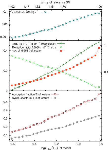
Figure 6: Absorption conditions for Si ii $\lambda 5972$.
Upper panel: Ratio of Si ii / Si iii ionisation fractions averaged over the shells.
Middle panel: $\langle\rho($Si ii$)\rangle$, excitation factor $\mathcal{E}_{l}$ and the resulting optical depth $\langle\tau\rangle_{l}$. $\langle\tau\rangle_{l}$ is roughly determined by $\langle\rho($Si ii$)\rangle$ and $\mathcal{E}_{l}$ $\left(\textrm{crudely }\langle\tau\rangle_{l}\propto\langle\rho(\textrm{Si\leavevmode\nobreak\ {\sc ii}})\rangle\cdot\mathcal{E}_{l}\right)$. $\langle\tau\rangle_{l}$ and $\mathcal{E}_{l}$ are plotted for one representative line ($\lambda 5958$); the data for the other doublet line are approximately proportional.
Lower panel: Absorption fraction $\mathfrak{A}$, and measured FD. Measurements in this and all following plots have been performed several times. Fluctuations in FD and also in $\mathfrak{A}$ (due to fluctuations in $\lambda_{F\>\!\!D}$) are represented by error bars (whenever large enough).

The Si ii $\lambda 5972$ absorption is stronger in dimmer SNe. This behaviour, which is the basis for the $\mathcal{R}$(Si ii) sequence, is due to the Si ii to Si iii ratio (Fig. 6, upper panel), which increases by a factor of $\sim\!\!100$ from luminous to dim SNe. Other ionisation stages are negligible in the layers probed.

The middle panel shows in detail the influence of the increasing Si ii density (crosses / dark, solid line) and of the excitation conditions on the optical depth. The fraction of ions in the lower level of the line ($\sim$ excitation factor, crosses / dashed line) decreases by $\sim\!\!90$% towards lower luminosities and temperatures. Yet, the optical depth of Si ii $\lambda 5972$ increases (filled squares / dotted line).

The absorption fraction $\mathfrak{A}$ (lower panel, open squares / dark, dotted line) increases towards lower luminosities, following the optical depth, as $\mathfrak{A}=\langle 1-\prod_{l}e^{-\tau_{l,k}}\rangle\approx\langle\sum_{l}\tau_{l,k}\rangle$ for small optical depths (first order). Measured line FDs (circles / grey line) reflect this trend.

The offset between the exact values of FD and the absorption fraction, which increases somewhat towards the dim end, is discussed in Appendix A. As it turns out, $\sim\!\!50\%$ of this offset is due to overlap with the emission part of the P-Cygni feature. The strength of this generally correlates with the absorption.

4.3 Si ii $\lambda 6355$ - a line with constant strength

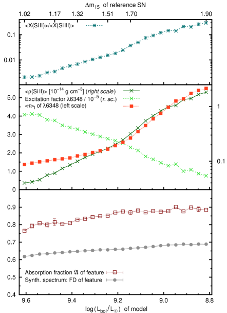
Figure 7: Absorption conditions for Si ii $\lambda 6355$; plot analogous to Fig. 6. The range of absorption fractions and FDs is small because of saturation. Apart from intrinsic line strengths, the physics behind Si ii $\lambda 5972$ and Si ii $\lambda 6355$ is similar. Minor differences depend on different blueshifts of the features (see Appendix B, Fig. 16): Si ii $\lambda 5972$ forms at $\gtrsim\!\!9000\$km s^-1 (luminous models) to $\sim\!\!8000\$km s^-1 (dim models); the stronger $\lambda 6355$ line always forms well above the photosphere at $\sim\!\!12500\$km s^-1.

Si ii $\lambda 5972$ evolves with luminosity, while Si ii $\lambda 6355$ does not (Fig. 7, bottom panel). This is due to saturation: because Si ii $\lambda 6355$ has large optical depths (middle panel), the absorption fraction (bottom panel) approaches unity, and it varies only weakly ($\mathfrak{A}=\langle 1-\prod_{l}e^{-\tau_{l,k}}\rangle\approx 1$ for large $\tau$). Measured FDs show a shallow trend, as do absorption fractions. The FD values indicate, however, an additional amount of residual flux. Again, we show in Appendix A that 50% of this amount is due to the P-Cygni emission.

4.4 Alternative explanations for $\textrm{{ FD}}(\textrm{Si\leavevmode\nobreak\ {\sc ii}\ }\lambda 5972)$ and $\mathcal{R}$(Si ii)?

Garnavich et al. (2004) suggested that the evolution of Si ii $\lambda 5972$ is due to a contribution of Ti ii lines in dim SNe. However, this possibility can be ruled out reviewing the list of active lines. In order for Ti ii lines to make a significant contribution, the Ti abundances must increase by a factor of $\gtrsim\!\!10$ in our SN 1999by model. This however leads to exceedingly large strengths for many other Ti lines (Fig. 8). We also do not find any further species that have a significant influence on the evolution of Si ii $\lambda\lambda 5972,6355$, with the possible exception of Na i in dim SNe (see Sec. 3.2).

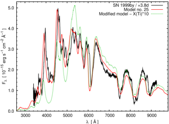
Figure 8: Model no. 25 and a modified version with 10-fold Ti abundance, where Ti lines contribute in the order of 10% to the strength of the 5972Å feature. A multitude of Ti ii transitions is active, with strongest lines at $\lambda\lambda$5888.89, 5910.05, 5987.39, 5994.94, 6001.4, 6012.75. $\textrm{{ FD}}(\textrm{Si\leavevmode\nobreak\ {\sc ii}\ }\lambda 5972)$ does not yet show an increase, also because Si ii $\lambda 5972$ gets weaker due to the slightly modified temperature structure. The larger Ti abundance leads, however, to an unrealistic opacity increase below $\sim\!\!5200$Å.

5 Discussion

5.1 Spectroscopic luminosity indicators: $\cal R$(Si ii) and Si ii $\lambda 5972$ line strengths

Having clarified the behaviour of observed FD values, we now briefly discuss the use of line strengths and ratios as luminosity indicators. We have shown that FD(Si ii $\lambda 5972$) correlates with luminosity and drives $\cal R$(Si ii). Thus, FD(Si ii $\lambda 5972$) itself (or similarly the equivalent width EW, as measured in Paper I) should be the most direct and meaningful luminosity indicator.

There are, however, uncertainties even in FD(Si ii $\lambda 5972$) as a spectroscopic luminosity indicator. First, the trend in the line is due to the combination of trends that are nonlinear in temperature, luminosity and also in $\Delta m_{15}(B)$ in the relevant ranges (see Sec. 4). In order to obtain luminosities from spectra, one has to choose an appropriate functional form (e.g. linear or second order) to fit the relation between feature strength and luminosity. Inaccuracies introduced by the use of such a functional form can easily be overlooked or misinterpreted as scatter. Second, intrinsic variations in the SNe and their spectra limit the precision of spectroscopic luminosity indicators. Differences in the abundance distributions among equally luminous SNe [see e.g. Tanaka et al. (2008), Mazzali & Podsiadlowski (2006)] are a possible reason for this (see also below, Sec. 5.2).

One way to reduce the error would be to use a number of spectroscopic luminosity indicators. Even quantities which are theoretically more elusive than FD may be useful, because different indicators respond differently to spectral peculiarities. Besides ratios like $\mathcal{R}$(Si ii), EW is also worth considering, because it accounts better for absorption in the line wings. SNe for which spectroscopic luminosity determination is unreliable could be identified if different indicators gave inconsistent luminosities.

The accuracy of spectroscopic luminosity determination could be improved if additional luminosity indicators were found that rely on species other than Si ii. A number of such quantities has already been defined (Nugent et al. 1995, Bongard et al. 2006, Paper I, Foley, Filippenko & Jha 2008). However, the validity of these potential luminosity indicators still needs to be critically assessed in terms of the physical differences among SNe with different luminosities (Mazzali et al., 2007).

5.2 FD(Si ii $\lambda 5972$) and SN physics

The Si ii $\lambda 5972$ optical depths, absorption fractions and FDs are quite tightly correlated. The line thus reflects the physics in the Si-dominated layers of most SNe Ia much better than Si ii $\lambda 6355$. It would be interesting to compare the Si ii $\lambda 5972$ profiles in $B$ max. spectra of several SNe with similar luminosity and explore the differences. If the Si distribution peaks in the zone with the largest Si ii ionisation fraction, one may expect relatively large FDs. On the other hand, a smeared-out Si distribution, or one with several peaks might cause an unusually shallow feature, as observed in SN 2006X [Wang et al. 2008, Elias-Rosa et al. 2008 (in prep.)].

Going one step further, it would be interesting to infer the distribution of Si using stratified abundance models (Stehle et al., 2005; Mazzali et al., 2008). This would be especially valuable in the context of SN Ia theory (see Mazzali et al. 2007) and explosion physics.

5.3 Other features evolving with luminosity

Apart from Si ii $\lambda 5972$ and $\lambda 6355$, other features in photospheric spectra of SNe Ia seem to evolve with luminosity. The Si ii $\lambda 4130$ line behaves similar to Si ii $\lambda 5972$ (Bronder et al., 2008), and the S ii trough is strongest for SNe with intermediate luminosity (Paper I). In Appendix B, these two features are investigated.

6 Conclusions

Based on a sequence of 25 synthetic spectra constructed to fit SNe Ia with different luminosities, we have been able to explain the $\mathcal{R}($Si ii$)-L$ relation.

The increasing strength of Si ii $\lambda 5972$ is responsible for the increase of $\mathcal{R}($Si ii$)$ from luminous to dim objects. This is in turn due to ionisation: in dimmer SNe, Si ii $\lambda 5972$ is stronger because the Si ii fraction increases more strongly than than the level occupation numbers decline. In contrast, Si ii $\lambda 6355$ is saturated because of its large optical depths. Thus, the line has a rather constant strength and only a minor influence on $\mathcal{R}($Si ii$)$.

An investigation as performed here shows how observed line strengths can be related to SN physics. Si ii $\lambda 5972$ probably provides the most reliable information about the Si layer in optical spectra.

If luminosity is to be inferred from spectra, a simultaneous evaluation of several line strengths or ratios is most promising. In order to find additional reliable luminosity indicators, one can apply our methods to further lines caused by single ions.

Appendix A The offset between fractional depths and absorption fractions

While the general trends in Si ii $\lambda 5972$ and $\lambda 6355$, and thus in $\mathcal{R}$(Si ii), can be explained by absorption effects, the mismatch between $\mathfrak{A}$ and $F\!\!\>D$ deserves closer investigation. Here, we analyse this offset.

A.1 Influences on the fractional depth besides absorption

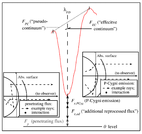
Figure 9: Contributions to the residual flux and continuum definitions. Insets: Definition of $F_{p}$ (packets penetrating the absorption surface without interaction) and of $F_{\epsilon,\textit{PCyg}}$ (packets having interacted with the multiplet and reached the observer afterwards). We term the remaining part of the emitted flux $F_{\epsilon}=F_{\epsilon,\textit{PCyg}}+F_{\epsilon,\textit{ad}}$ “additional reprocessed flux” ($F_{\epsilon,\textit{ad}}$).

There are two potential reasons for a difference between absorption fraction and FD: First, photons may be shifted into the observed wavelength of a feature in re-emission processes, and enhance the residual flux. Second, the estimated pseudo-continuum may deviate from the flux behind the absorption surfaces, as seen from the observer.

To trace these effects, we counted photon packets representing different components of the residual flux in our simulations and recorded the pseudo-continuum estimate for each FD measurement.

Components of the residual flux

The residual flux at a measurement wavelength $\lambda_{F\>\!\!D}$ can be split into contributions of different origin (Fig. 9).

One contribution (“penetrating flux” $F_{p}$) directly depends on the absorption fraction $\mathfrak{A}$. It consists of photons crossing the multiplet’s absorption surfaces without being absorbed, and is approximately given by

$$F_{p}\!\approx\!(1-\mathfrak{A})F_{EC}$$ (5)

where $F_{EC}$ (“effective continuum”) is the flux impinging on the absorption surfaces of the multiplet, multiplied by a correction factor. This factor, usually a bit smaller than unity, accounts for the fact that photons passing the absorption surface do not have a 100% chance of escaping the envelope.

The rest of the residual flux (“emission” $F_{\epsilon}$) consists of photons which have been shifted to an observer-frame wavelength $\sim\!\!\lambda_{F\>\!\!D}$ at the absorption surfaces (corresponding to $\lambda_{F\>\!\!D}$) or even closer to the observer. In the following, photons that underwent absorption and reemission at the absorption surfaces will be called “P-Cygni emission” ($F_{\epsilon,\textit{PCyg}}$). The amount of P-Cygni emission will generally correlate with the absorption strength. The flux of photons that were reprocessed into an observer-frame wavelength $\sim\!\!\lambda_{F\>\!\!D}$ (for example in line processes) at depths closer to the observer will be called “additional reprocessed flux” ($F_{\epsilon,\textit{ad}}$). It is an upper limit estimate for the flux that enters the feature without correlation to the absorption conditions.

The relation between $\mathfrak{A}$ and FD

In general, the relation between absorption fraction, emission and measured residual flux $\frac{F_{\textrm{res}}}{F_{PC}}=1-FD$, is:

$$\frac{F_{\textrm{res}}}{F_{PC}}\equiv(1-FD)\!=\!\frac{F_{p}\!+\!F_{\epsilon}}{F_{PC}}\Bigg{|}_{\!\lambda_{\!F\>\!\!D}}\!\!\!\!\!\!\!\approx\!(1-\mathfrak{A})\frac{F_{EC}}{F_{PC}}+\frac{F_{\epsilon}}{F_{PC}}.$$ (6)

$\mathfrak{A}$ and FD are closely related only if $\frac{F_{EC}}{F_{PC}}$ and the additional reprocessed flux are roughly constant with luminosity. As the data will show, this is the case for Si ii $\lambda 5972$ and $\lambda 6355$, but not always for the lines discussed in Appendix B.

A.2 Si ii $\lambda 5972$

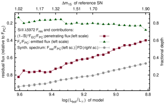
Figure 10: Contributions to the emission, and FD for Si ii $\lambda 5972$. All fluxes are given relative to the pseudo-continuum. The penetrating flux $(1-\mathfrak{A})\!\times\!\frac{F_{EC}}{F_{PC}}$ and the emitted flux $\frac{F_{\epsilon}}{F_{PC}}$ can be added up on the left scale to obtain a prediction for the residual flux (not explicitly shown). This coincides roughly with the measured residual flux (grey curve). The grey curve represents the fractional depth with units on the right hand side.

For Si ii $\lambda 5972$, emission causes a moderate offset between penetrating flux and measured residual flux $F_{\textrm{res}}=1-\textrm{ FD}$ (Fig. 10, squares / dark line and circles / grey line, respectively). On average, about half of the emission (triangles / dark, dotted line) is P-Cygni emission, which increases with decreasing luminosity. The additional reprocessed flux, in turn, is relatively constant (not explicitly shown), as is $\frac{F_{EC}}{F_{PC}}$. Thus, the measured FDs correlate well with the absorption fractions.

Still, the offset between FDs and absorption fractions has a practical consequence: It makes the relative decrease in FD from intermediate to very luminous SNe larger, increasing the influence of Si ii $\lambda 5972$ on $\mathcal{R}$(Si ii).

A.3 Si ii $\lambda 6355$

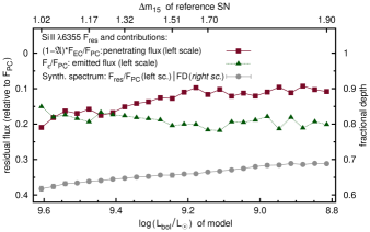
Figure 11: Emission contributions and FD for Si ii $\lambda 6355$; plot analogous to Fig. 10.

Intuitively, the residual flux in the saturated Si ii $\lambda 6355$ line should be lower than observed. Again, this is in roughly equal parts due to P-Cygni emission and the additional reprocessed flux. Both these contributions and $\frac{F_{EC}}{F_{PC}}$ are practically constant within the luminosity sequence.

A.4 Concluding remarks

For the two lines determining $\mathcal{R}$(Si ii), $\frac{F_{EC}}{F_{PC}}$ is constantly $\approx\!1$ and the additional reprocessed flux is small ($\lesssim\!\!10\%$ of the residual flux). Even under slightly different simulation conditions, we expect FDs to correlate well with the absorption in their respective lines, because redwards of Si ii $\lambda 5972$, the number of lines which might cause deviations is relatively small.

Appendix B Investigation of further features (Si II 4130Å, S II 5640Å)

SN Ia spectra contain a wealth of features, of some of which show evolution with luminosity (see e.g. Nugent et al. 1995 and Paper I). Calcium absorptions frequently seem to suffer from saturation and high-velocity contributions (Hatano et al., 1999; Mazzali et al., 2005; Tanaka et al., 2006). Interesting trends have been found for Si ii $\lambda 4130$ and the S ii “W-trough”: Si ii $\lambda 4130$ correlates with luminosity like Si ii $\lambda 5972$ (Bronder et al., 2008), although the Si ii $\lambda 4130$-luminosity correlation suffers from more scatter (Bronder et al. 2008, Fig. 10). The S ii trough, in contrast, shows a parabolic trend, with largest strength at intermediate luminosities (Paper I). Both features are largely caused by a single ion and can be investigated with the technique applied to $\mathcal{R}$(Si ii).

B.1 Si ii $\lambda 4130$: a supplementary luminosity indicator

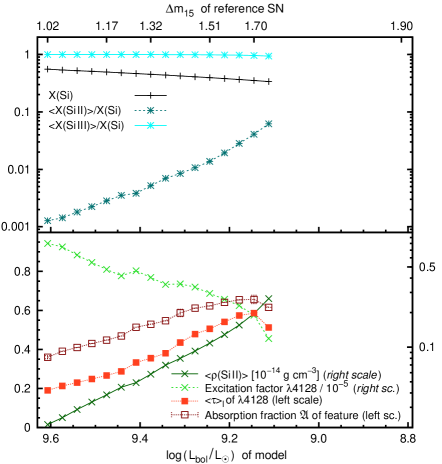
Figure 12: Absorption conditions for Si ii $\lambda 4130$ (for $\log(L_{\textrm{bol}}/L_{\odot})\gtrsim\!\!9.1$, see text).
Upper panel: Ionisation and abundance trends: Si mass fraction, and Si ii and Si iii ionisation fractions (shell-averaged).
Lower panel: $\langle\rho($Si ii$)\rangle$ and excitation factor $\mathcal{E}_{l}$; $\langle\tau\rangle_{l}$ and absorption fraction $\mathfrak{A}$. $\langle\tau\rangle_{l}$ and $\mathcal{E}_{l}$ are plotted for one representative line ($\lambda 4128$); the data for the other triplet lines are approximately proportional.

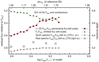
Figure 13: Contributions to the emission, and measured residual flux (grey curve) for Si ii $\lambda 4130$. The grey curve represents the fractional depth with units on the right hand side. Measurements of the residual flux in the observed reference spectra are shown for comparison.

The data for this feature are summarised in Figs. 12 and 13. The line can be measured only in spectra with $\log(L/L_{\odot})\!\!\gtrsim\!\!9.1$. At lower luminosities, the Ti ii lines at $\sim$4000-4300Å typical of dim SNe affect the feature.

Among normal SNe, the absorption fraction shows a trend similar to Si ii $\lambda 5972$ (Fig. 12, lower panel). Measured FD values (Fig. 13, circles) correlate with the absorption fractions, but increase only slowly towards lower luminosities. This is mainly due to an increase in the additional reprocessed flux (not explicitly shown), which leads to an increase in the emission (triangles / dark, dotted line). Contamination effects (e.g. by S ii $\lambda 4162.7$, Ni ii $\lambda 4067.0$ and Co ii $\lambda 4160.7$) are a possible reason for this.

As noted by Bronder et al. (2008), the Si ii $\lambda 4130$ strength could be used as a luminosity indicator for intermediate to bright objects. However, FD does not follow the absorption fraction very well for the feature. Thus, the relation between luminosity and Si ii $\lambda 4130$ line strength shows large scatter [Bronder et al. (2008), Fig. 10], and we regard the feature as a supplementary luminosity indicator at most.

B.2 S ii $\lambda 5640$: a mix of temperature and abundance trends

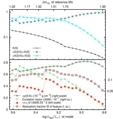
Figure 14: Absorption conditions for S ii $\lambda 5640$ (red part of W-trough). Abrupt variations in the values are due to jumps in the measurement positions (see Fig. 16).
Upper panel: S mass fraction of our models, and S ii and S iii ionisation fractions (shell-averaged).
Lower panel: $\langle\rho($S ii$)\rangle$ and excitation factor $\mathcal{E}_{l}$; $\langle\tau\rangle_{l}$ and absorption fraction $\mathfrak{A}$. $\langle\tau\rangle_{l}$ and $\mathcal{E}_{l}$ are plotted for one example line (lower level 13.7eV, non-metastable). The lines of the S ii $\lambda 5640$ multiplet originate from different levels at $\sim$13.7…14eV, including a metastable one. Trends in $\langle\tau\rangle_{l}$ values for other lines will thus deviate somewhat, causing the absorption fraction to deviate from the individual optical depth trends.

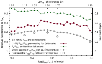
Figure 15: Emission contributions and FD for S ii $\lambda 5640$. Plot analogous to Fig. 13.

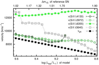
Figure 16: Line-of-sight velocities corresponding to $\lambda_{F\>\!\!D}$ values (in the synthetic spectra) for all features discussed in this paper. Weaker features tend to form near the photosphere at lower velocities, and trace the photospheric recession (filled squares / black, dashed line).

The blue part of the S ii W-trough has different depths in the synthetic and observed spectra (Fig. 1, see also Kotak et al. 2005). Thus, we chose to investigate only the red component (lines/multiplets $\lambda\lambda 5606,5640$). The pseudo-continuum was set as if the whole trough were measured.

The results are shown in Figs. 14 and 15. Sulphur has different level structures and a lower ionisation threshold than silicon, so that the S ii/S iii ratio is always $>\!\!0.5$. Furthermore, because of the steeply declining line velocity (Fig. 16), the temperatures in the layers probed do not vary as much as for the Si lines within the sequence.

In the range from large to intermediate SN luminosity, a mild increase in the S ii fraction (Fig. 14, upper panel, asterisks / dark, dashed line) increases the optical depths somewhat. At low luminosities, the S ii fraction approaches 100%, so that decreasing S abundances (Fig. 14, upper panel, crosshairs / solid line) and level occupation numbers lead to a decreasing absorption strength (Fig. 14, lower panel).

The resulting FDs (Fig. 15, circles) in the synthetic spectra increase from large to intermediate luminosities and then decline again, similar to the parabolic trend in Paper I for the $EW$ of the W-trough. The decline in FD from intermediate- to low-luminosity SNe is amplified by an increase in the additional reprocessed flux, which affects dim SNe more strongly (triangles / dark, dotted line).

References

- Abbott & Lucy (1985) Abbott D. C., Lucy L. B., 1985, ApJ, 288, 679
- Arnett (1982) Arnett W. D., 1982, ApJ, 253, 785
- Benetti et al. (2004) Benetti S. et al., 2004, MNRAS, 348, 261
- Bongard et al. (2006) Bongard S., Baron E., Smadja G., Branch D., Hauschildt P.H., 2006, ApJ, 647, 513
- Bronder et al. (2008) Bronder T. J. et al., 2008, A&A, 477, 717
- Burstein & Heiles (1982) Burstein D., Heiles C., 1982, AJ, 87, 1165
- Conley et al. (2006) Conley A. et al., 2006, AJ, 132, 1707
- Elias-Rosa et al. (2008) Elias-Rosa N. et al., 2008, in preparation
- Filippenko et al. (1992) Filippenko A. V. et al., 1992, ApJ, 384, L15
- Foley, Filippenko & Jha (2008) Foley R. J., Filippenko A. V., Jha S. W., 2008, arXiv:0803.1181 [astro-ph]
- Garnavich et al. (2004) Garnavich P. et al., 2004, ApJ, 613, 1120
- Hachinger, Mazzali & Benetti (2006) Hachinger S., Mazzali P. A., Benetti S., 2006, MNRAS, 370, 299 (Paper I)
- Hatano et al. (1999) Hatano K., Branch D., Fisher A., Baron E., Fillippenko A. V., 1999, ApJ, 525, 881
- Hillebrandt & Niemeyer (2000) Hillebrandt W., Niemeyer J. C., 2000, ARA&A, 38, 191
- Kotak et al. (2005) Kotak R. et al., 2005, A&A, 436, 1021
- Lucy (1999) Lucy L. B., 1999, A&A, 345, 211
- Mazzali (2000) Mazzali P. A., 2000, A&A, 363, 705
- Mazzali & Lucy (1993) Mazzali P. A., Lucy L. B., 1993, A&A, 279, 447
- Mazzali & Podsiadlowski (2006) Mazzali P. A., Podsiadlowski P., 2006, MNRAS, 369, L19
- Mazzali et al. (1993) Mazzali P. A., Lucy L. B., Danziger I. J., Gouiffes C., Cappellaro E., Turatto M., 1993, A&A, 269, 423
- Mazzali et al. (2001) Mazzali P. A., Nomoto K., Cappellaro E., Nakamura T., Umeda H., Iwamoto K., 2001, ApJ, 547, 988
- Mazzali et al. (2005) Mazzali P. A. et al., 2005, ApJ, 623, L37
- Mazzali et al. (2007) Mazzali P. A., Röpke F. K., Benetti S., Hillebrandt W., 2007, Sci, 315, 825
- Mazzali et al. (2008) Mazzali P. A., Sauer D. N., Pastorello A., Benetti S., Hillebrandt W., 2008, MNRAS, doi:10.1111/j.1365-2966.2008.13199.x
- Nomoto, Thielemann & Yokoi (1984) Nomoto K., Thielemann F.-K., Yokoi K., 1984, ApJ, 286, 644
- Nugent et al. (1995) Nugent P., Phillips M., Baron E., Branch D., Hauschildt P., 1995, ApJ, 455, L147
- Patat et al. (1996) Patat F., Benetti S., Cappellaro E., Danziger I. J., della Valle M., Mazzali P. A., Turatto M., 1996, MNRAS, 278, 111
- Pauldrach et al. (1996) Pauldrach A. W. A., Duschinger M., Mazzali P. A., Puls J., Lennon M., Miller D. L., 1996, A&A, 312, 525
- Phillips (1993) Phillips M. M., 1993, ApJ, 413, L105
- Riess et al. (1999) Riess A. G. et al., 1999, AJ, 118, 2675
- Röpke & Hillebrandt (2005) Röpke F. K., Hillebrandt W., 2005, A&A, 431, 635
- Schlegel, Finkbeiner & Davis (1998) Schlegel D. J., Finkbeiner D. P., Davis M., 1998, ApJ, 500, 525
- Stanishev et al. (2007) Stansihev V. et al., 2007, A&A, 469, 645
- Stehle et al. (2005) Stehle M., Mazzali P. A., Benetti S., Hillebrandt W., 2005, MNRAS, 360, 1231
- Tanaka et al. (2006) Tanaka M., Mazzali P. A., Maeda K., Nomoto K., 2006, ApJ, 645, 470
- Tanaka et al. (2008) Tanaka M. et al., 2008, ApJ, 677, 448
- Taubenberger et al. (2008) Taubenberger S. et al., 2008, MNRAS, 385, 75
- Wang et al. (2008) Wang X. et al., 2008, ApJ, 675, 626