Synergetics and Its Application to Literature and Architecture

Abstract

A series of phenomena pertaining to economics, quantum physics, language, literary criticism, and especially architecture is studied from the standpoint of synergetics (the study of self-organizing complex systems). It turns out that a whole series of concrete formulas describing these phenomena is identical in these different situations. This is the case of formulas relating to the Bose–Einstein distribution of particles and the distribution of words from a frequency dictionary. This also allows to apply a “quantized” from of the Zipf law to the problem of the authorship of Quiet Flows the Don and to the “blending in” of new architectural structures in an existing environment.

1 Nonlinear addition and synergetics

Let us begin with the description of the Kolmogorov axioms for nonlinear addition, which we will supplement by an additional axiom.

A sequence of functions $M_{n}$ determines a regular type of mean if the following conditions are satisfied (Kolmogorov).

I.   $M(x_{1},x_{2},\dots,x_{n})$ is continuous and monotone in each variable. To be definite, we assume that $M$ is monotone increasing in each variable.

II.   $M(x_{1},x_{2},\dots,x_{n})$ is a symmetric function.

III.  The mean of identical numbers is equal to their common value: $M(x,x,\dots,x)=x$.

IV.   A group of values can be replaced by their own mean without changing the entire mean:

$$M(x_{1},\dots,x_{m},y_{1},\dots,y_{n})=M_{n+m}(x,\dots,x,y_{1},\dots,y_{n}),\quad\text{where}\quad x=M(x_{1},\dots,x_{n}).$$

  Theorem 1

(Kolmogorov). If conditions I–IV are satisfied, then the mean $M(x_{1},x_{2},\dots,x_{n})$ has the form

$$M(x_{1},x_{2},\dots,x_{n})=\psi\Big{(}\frac{\varphi(x_{1})+\varphi(x_{2})+\dots+\varphi(x_{n})}{n}\Big{)},$$ (1)

where $\varphi$ is a continuous strictly monotone function, while $\psi$ is its inverse.

For the proof, see [2].

It is rather obvious that any stable system must also satisfy the following axiom, which is added to the Kolmogorov axiomatics [3].

V.   If to all the $x_{k}$ we add the same value $\omega$, then the mean will increase by the same value $\omega$.

There exists a unique family of nonlinear functions satisfying axiom V. It has the form

$$\varphi(x)=A\exp(\beta x)+B,$$ (2)

where $A,\beta\neq 0$, $B$ are numbers not depending on $x$.

Accordingly, the new addition of elements $a>0$ and $b>0$ is defined by the formula

$$a\oplus b=\frac{1}{\beta}\ln(e^{\beta a}+e^{\beta b}).$$ (3)

and the $\beta$-mean is

$$\frac{a\oplus b}{2}=\frac{1}{2\beta}\ln(e^{\beta a}+e^{\beta b}).$$ (4)

Now we have obtained a family depending on the parameter $\beta$, which for $\beta=0$ gives us the usual arithmetic, according to which, in the biblical story described at the beginning of this article, each brings the same amount of wine, while when $\beta\to\infty$ everyone brings water:

$$\lim_{\beta\to\infty}a\overset{\beta}{\to}\oplus b=\min(a,b).$$

The arithmetic thus obtained led to the appearance of idempotent analysis and tropical mathematics, now rapidly developing (see [4], chap. 2; [5], sec. 9; [6], sec. 5.1).

The new arithmetic, which depends on the parameter $\beta$, yields in the case of a large number of summands, formulas very similar to those of thermodynamics. The parameter $\beta$ has the physical meaning of $1/T$, where $T$ is the temperature. However, the corresponding phase transition was not noticed by physicists. In the works [7, 8], it was called phase transition of the zeroth kind. Below we will discuss this notion in more detail.

One of the fathers of synergetics, G. Haken, in his article [9], recalls the following story from the Ancient Testament: “It was the custom in a certain community for the guests to bring their own wine to weddings, and all the wines were mixed before drinking. Then one guest thought that if all the other guests would bring wine, he would not notice when drinking if he brought water instead. Then the other guests did the same, and as the result they all drank water.”

In this example, two situations are possible. In the first, everyone contributes his share, giving his equal part, and everyone will equally profit. In the second, each strives for the most advantageous conditions for himself. And this can lead to the kind of result mentioned in the story.

Two different arithmetics correspond to these two situations. One arithmetic is the usual one, the one accepted in society, ensuring “equal rights,” and based on the principle “the same for everyone,” for instance in the social utopia described by Owen. In a more paradoxal form, this principle is expressed in M. Bulgakov’s Master and Margarita by Sharikov: “Grab everything and divide it up.”

The aspiration to this arithmetic is quite natural for mankind, but if society is numerous and non-homogeneous, then it can hardly be ruled according to this principle. The ideology of complete equality and equal rights, which unites people and inspires to perform heroic deeds, can effectively work only in extremal situations and for short periods of time. During these periods such an organization of society can be very effective. An example is our own country, which, after the destructions and huge losses of World War II, rapidly became stronger than before the war.

One of the authors personally witnessed such an atmosphere of psychological unity when he was working on the construction of the sarcophagus after the catastrophe of the Chernobyl nuclear facility. The forces of the scientists involved were so strongly polarized that the output of each of them was increased tenfold as compared to that in normal times. During that period it was not unusual for us to call each other in the middle of the night.

Nevertheless such heroism, self-denial, and altruism, when each wants to give (and not to take) as much as possible, is an extremal situation, a system that can function only for short intervals of time. Here the psychological aspect is crucial, everyone is possessed by the same idea — to save whatever may be saved at any cost. But the psychology of the masses, which was studied by the outstanding Russian emigré sociologist Pitirim Sorokin, is presently studied only outside of Russia.

A similar enthusiasm takes hold of the masses during revolutions. Thus, the October revolution in our country and the Great Chinese revolution led the masses involved in the revolutionary process to believe that they can “move mountains.” Nevertheless the policy of military communism in Russia and the policy of the great leap forward in China were doomed to failure.

In order for the system to survive, it was necessary to implement a different “egoistical” arithmetic — the NEP (New Economic Policy) arithmetic. In China a similar arithmetic was in fact introduced by Deng Siao Ping and his group.

This arithmetic is just as simple as ordinary school arithmetic but, unfortunately, it is not studied in school.

The old arithmetic was linear, as the Soviet song goes “We all live happily, divide all things equally,” whereas the new arithmetic is that of nonlinear addition. And although it does not seem objective, this arithmetic leads to certain rules which ensure the establishment of equilibrium, the system becomes self-organizing. Such an equilibrium exists, for instance, in living nature. Everything follows the order of things (certain animals eat other animals, a third group feeds on the first one and so on), but, as we know, cataclysms also occur in nature.

The practice of corruption has been established in Russian society. It is a self-organizing system. A person yields power and enjoys wide opportunities. If the state were not to provide him with benefits, he would obtain them from the people whom he helps.

We have attempted to describe, on the basis of this new arithmetic, both the equilibrium state of the system and the catastrophic states that may occur. Equilibrium may last for a long time, but progressively revolutions may arise. In order to avoid catastrophic phenomena, during which the nonlinear arithmetic explodes in a burst and is replaced by the ordinary arithmetic, the political system of the state must be sufficiently flexible.

As an example, let me mention the progressive implementation of racial equality in the USA for Afro-Americans, which lasted for approximately 30 years. If we look at this situation without bias, then it is similar to the one described in I. Erenburg’s grotesque novel “DE Trust.” Of course, clashes and even killings occurred, but overall the system survived without serious cataclysms.

On the other hand, completely equalitarian systems, as we see from historical examples, are usually extremely cruel to separate individuals. Even the strongest and most natural feeling of love can be severely repressed by such a system.

Let us recall the Russian rebel Stepan Razin, who was forced to throw his beautiful wife overboard at the highest point of his love. Stepan Razin was a rebel leader with colossal authority. But the structure of which he was the leader demanded that he perform this sacrifice and crime, and he complied. Another example is the anarchist rule under the authority of the military commander and agitator Nestor Makhno. When Makhno married his great love (Vasetskaya) and their child was born, his cronies arrested his wife and baby and forced them into exile under the threat of death. Makhno suffered terribly, but did not leave his comrades-in-arms.

One of the authors has also studied the very tenacious anarcho-communist regime of Pol Pot and Chang Sari in Cambodia. Under that regime marriages were impossible unless approved by the communist cell of the bride-to-be. Following an assessment of the qualities and faults of the potential wife, the bridegroom was either allowed or forbidden to marry her, and another prospective bride could be assigned.

In a similar way, during the war, military commanders could be extremely cruel to young recruits experiencing the psychologically very natural feeling of fear. In Cambodia, everyone ate at the same table, and if someone, even a child, ate more than his share, he would be severely punished. In the same way, in Russia during the period of military communism, it was considered wrong not to denounce anyone attempting to appropriate state-owned resources (e.g., to steal a paper clip from one’s office). In contrast to this, at the present time, it is considered shameful to inform the authorities, say, of a neighbor who sublets an apartment without paying the corresponding city taxes.

Specialists in synergetics study problems related to revolutions (see, for example, [10]) and work on systems of preemptive warning. Working on the economic problems set before him by the industrialist I.Silaev (Deputy Chairman of the Council of Ministers of the USSR, and later Chairman of the Council of Ministers of the Russian Soviet Federative Socialist Republic), one of the present authors and his specially recruited group of collaborators developed such a system (see [11, 12]). However, this system was not supported by the subsequent government and the group working on the problem was dissolved. As a result, seven days before the 1991 putsch (which led to the disintegration of the USSR), an article entitled “How to avoid a total catastrophe” was published by the daily Izvestia. The warning explained in the article was obtained via a computerized mathematical program.

All the collaborators were highly qualified experts and most of them soon found jobs in foreign corporations and institutes.

Now about history as a science. What is history? Suppose that a person writes down the events of his life in a diary. Small discrepancies from the uniform flow of life may be extremely annoying for this person, but by the end of the day they may be forgotten, small squabbles may then seem insignificant. If the person compiles his diary only at the end of the week, and not right after each event, his memory keeps only the important, the essential ones, while to the lesser ones he no longer pays heed. The same happens in the “averaged” economics. Prices in the stock exchange jump very rapidly. These jumps depend on unimportant events, on small political changes, but on the average the economy evolves slowly, until a default, a crisis, or a revolution occurs. Thermodynamical equilibrium also describes the evolution of a system in time, but at small temperatures of the system it “waits” until things “level off,” and only then “records in its diary” slightly changed state of the system. However, abrupt phase transitions sometimes occur. It turns out that there exist common laws governing all these quasi-equilibrium states, namely the laws of synergetics.

Let us recall that a phase transition of the first kind for physical processes is the transformation of matter from one state to another (water to ice, water to vapor, etc.) during which the volume and heat energy undergoes a jump, but there is no jump in the “kinetic” energy. For example, water freezes at 0 degrees Celsius and boils at 100. However, in the interval between 0 and 100 degrees, there exists a threshold temperature above which it is impossible to save ice under any conditions. One can only approach it. It is this threshold temperature that was called temperature of the phase transition of the zeroth kind.

If this phase transition occurs, a large amount of “kinetic” energy is freed. For classical liquids, such a phase transition has never been carried out in practice. It can only happen for quantum liquids. From the mathematical viewpoint, phase transitions of the zeroth kind in the thermodynamics of quantum liquids, economic defaults, and revolutions in society are phenomena of the same type. Namely, there is a limiting “temperature” of social tension such that, whenever it is reached, there is no way that the revolutionary process can be stopped; see [12].

Surprising as it may seem, any model of society, primitive or complex, based on the $\beta$-arithmetic, leads, from the mathematical point of view, to the same phase transition of the zeroth kind, characterized by the freeing of kinetic energy and branching of exactly the same type as in physics.

The fountain (burst) that accompanies this phase transition is bloodletting, the “fountain of blood” produced by the French revolution as it conquered huge territories. The hopes of the left-wing bolsheviks for a world revolution were not realized (their “fifth column” in the Antante was not strong enough) and the kinetic energy (the burst) gushed only in the one huge country.

But how must one choose the parameter $\beta$ (i.e., the temperature), so as to achieve equilibrium, some sort of egalitarianism, without carrying it too far?

It turns out that one can state a law called the lack of preference law for a large number of “distributed advantages,” which will allow avoiding catastrophes for long enough. And we shall see below that this law works in nature, in language, in the organization of web sites, and in document systems, and there is some hope that it may be implemented in our shaky society.

2 The salary model

Consider the following simple model. A personnel of $N$ persons can receive the monthly salary of $\lambda_{1},\lambda_{2},\dots,\lambda_{n};\;\lambda_{i}>\lambda_{i-1}$.

The number of positions with salary $\lambda_{i}$ equals $Q/{i^{s}}$, where $Q$ is sufficiently large, $s\geq 0$.

The number of positions with given salary decreases as salary increases.

Denote by $N_{i}$ the number of people receiving the salary $\lambda_{i}$. The total expenditure on salaries is $\sum N_{i}\lambda_{i}$. This number must not exceed the budget $E$,

$$\sum N_{i}\lambda_{i}\leq E.$$ (5)

We will assume that all possible distributions of the personnel among the $\sum_{i=1}^{n}Q/{i^{s}}$ positions is equiprobable.

What distribution $N_{i}$ is most probable and what is the probability of deviation from this most probable number as $N\to\infty,\,E\to\infty,\,n\to\infty$?

It turns out that the density of probability of the distribution of $N_{i}$ satisfies the relation

$$\frac{N_{i}}{Q}=i^{s}\frac{1}{e^{\beta(\lambda_{i}+\delta)}-1},$$ (6)

where $\beta$ and $\delta$ can be determined from the relation

$$\sum i^{s}\frac{1}{e^{\beta(\lambda_{i}+\delta)}-1}=N,\qquad\sum i^{s}\frac{\lambda_{i}}{e^{\beta(\lambda_{i}+\delta)}-1}=E.$$ (7)

The relation (6) is similar to the Bose–Einstein distribution law. Here $\beta$ is the same as the one appearing in the definition of the new arithmetic. This will be established below. Thus the parameter $\beta$ is determined from a certain new equilibrium principle for all the situations considered, the self-organization principle.

The papers [13, 14] give the exact formulation of the corresponding theorem, which encompasses the physical situations as well as the ones coming from the humanities and the social sciences.

First let us note the following physical phenomenon for “weakly nonideal Bose gas,” namely, the Allen–Jones effect for liquid helium-4. If we make a small hole in a narrow (of diameter $10^{-4}$) tube through which liquid helium is flowing and raise the temperature of that part of the tube to the critical level of phase transition of zeroth kind, then a fountain (a gerbe or burst) of height up to 14 cm sprouts from the aperture near the point of heating. This effect, discovered in 1938 by D. Allen and H. Jones, is known as the fountain effect.

We shall assume that the real salary in the previous salary model decreases linearly with the increase of the number of employees. The coefficient of this decrease is $1/N$, hence any nonlinear decrease in the leading term yields a linear one.

In this case, we obtain a mathematical picture coinciding with the one appearing in the liquid helium-4 experiment, and for an appropriate choice of the parameter $\beta$, a phase transition of zeroth kind occurs.

Let us compute the mean salary using the $\beta$-mean. Denote

$$q_{i}=Q/{i^{s}}.$$

The number of different possibilities in which the number of employees receiving the salary $\lambda_{i}$ was $N_{i}$ can be calculated by using the formula

$$\gamma_{i}(k_{i})=\frac{(k_{i}+g_{i}-1)!}{k_{i}!(g_{i}-1)!}\,;$$ (8)

$$Q=\sum_{i=1}^{n}g_{i},$$ (9)

$$M(\beta,N)=\frac{1}{\beta N}\ln\bigg{(}\frac{N!(G-1)!}{(N+G-1)!}\sum_{\{k_{i}=N\}}\gamma(\{k\})\exp\left(\beta{\cal B}(\{k\})\right)\bigg{)}.$$ (10)

The mean salary is

$$M(\beta,N)=\frac{1}{\beta N}\ln\biggl{(}\frac{N!(G-1)!}{(N+G-1)!}\sum_{\{N_{i}\}_{\sum N_{i}=N}}\gamma_{i}(N_{i})e^{\beta\lambda_{i}N_{i}}\biggr{)}.$$ (11)

Invoking Stirling’s formula and the Laplace method, we can establish the connection of this mean as $N\to\infty$ with the density of the distribution (6) [15].

In our example, we assumed that $q_{i}=i^{-s}Q$. Let us present the argument in the general case.

3 Dimension

It is well known that the integration in spherical coordinates over the space $\mathbb{R}^{n}$ leads to the density $r^{n-1}$, where $r$ is the radius of the $k$-dimensional sphere. Similarly, as shown by Yu. Manin, to the fractional or negative dimension $D$ corresponds the density $r^{D-1}$.

The dimension of the space underlying a problem, as a rule, is determined from the experiment or from some indirect considerations. For example, the dimension of the point-like presentation of a photograph (its digital version), like a pointillist painting, is obviously of dimension zero, which yields $s=D-1=-1$.

G. Haken wrote that, in his opinion, an important role in uncovering the causes of self-organizing systems must be played by objects which simultaneously possess a quantum and a classical structure. Such an object is, in particular, the quantum oscillator. In it, the quasi-classical structure reduces to finding an exact solution and performing a change of variables. One can get rid of $h$, the Planck constant. Namely, for the equation

$$-\frac{h^{2}}{2m}\Psi^{{}^{\prime\prime}}_{xx}+\omega^{2}x^{2}\Psi=E_{n}\Psi,$$ (12)

where the $E_{n}$ are eigenvalues, $\omega,m$ are constants (frequency and mass), the substitution

$$x=\big{(}{\sqrt{h}}\big{/}{\root 4 \of{2m}}\,\big{)}y$$

yields the equation

$$-\Psi^{{}^{\prime\prime}}_{yy}+\omega^{2}y^{2}\Psi=\lambda_{n}\Psi,\quad\lambda_{n}=\frac{2mE_{n}}{h}-\frac{1}{2}.$$ (13)

Let us put $\omega=1$; then $\lambda_{n}=n$.

Consider the line, the plane, and $3$-space. On the line, we pick the points $i=0,1,2,\dots$, on the $x,y$-plane the points $(x,y)$, where $x=i=0,1,2,\dots$;  $y=j=0,1,2,\dots$ To this set of points $(i,j)$ let us assign points on the line (natural numbers) $l=1,2\dots$

To each point assign all the pairs of points $i$ and $j$ such that $i+j=l$. The number of such pairs is $l+1$. On the $z$-axis let us put $z=k=0,1,2,\dots$ so that $i+j+k=l$. Then the number $n_{i}$ of points in 3-space will be

$$n_{l}=\frac{(l+1)(l+2)}{2}.$$

In the first year of the 20th century Planck quantized the energy of the oscillator, assuming that it changes by whole numbers (multiplied by a parameter $h$, now known as the Planck constant).

If in formula  (11), we set $\lambda_{i}=i$, then in the three-dimensional case to each $i$ will correspond a collection of ${i(i+1)}/2$ equal values $\lambda_{i}=i$ (they are the multiplicities or “degeneracies” of the oscillator’s spectrum). The formula  (7) in this particular case can be written as

$$N_{l} =\text{const}\sum_{i=0}^{l}\frac{(i+1)(i+2)}{2(e^{\beta i+\sigma}-1)};$$ (14)

$$\Delta N_{l} =\text{const}\frac{i(i+1)}{2(e^{\beta i+\sigma}-1)}\quad\text{for large}\quad i,$$

$$dN =\text{const}\frac{\omega^{2}d\omega}{e^{h\omega\beta}-1}$$

(compare with formula (60.4) from [16]).

Here the weight $\omega^{2}$ coefficient is derived by Landau and Lifshits from the fact that our space is three-dimensional.

It is more logical to argue differently. It is easy to verify, in the $D$-dimensional case, that the sequence of weights (multiplicities) of the number of variants $i=\sum_{k=1}^{D}m_{k}$, where $m_{k}$ are arbitrary natural numbers, have the form

$$q_{i}(D)=\mathop{\rm const}\nolimits\frac{(i+D-2)!}{(i-1)!D!},$$ (15)

and this constant depends on $D$.

For any $D$, we have

$$N_{l}=\mathop{\rm const}\nolimits\sum_{i=1}^{l}\frac{q_{i}(D)}{e^{\beta i}-1}.$$ (16)

Comparison with experimental data shows that $D=3$, and so we may conclude that photons “live” in three-dimensional space, and not in four-dimensional Minkowski space, as one might have assumed.

Thus, for natural numbers, we have the sequence of weights $q_{i}$ (or simply the weight) of the form  (15).

It is known that some sets may have a non-integer dimension (some attractors, fractals, the Sierpinski rug, etc.).

It is easy to continue the sequence of weights $q_{i}$ to the general case by replacing the factorials by the $\Gamma$-function:

$$q_{i}(D)=\mathop{\rm const}\nolimits\frac{\Gamma(D+i-1)}{\Gamma(i)\Gamma(D+1)}.$$ (17)

Let us pick a negative $D$. This is the negative dimension of space.

Suppose some person came into a huge inheritance $Q$ in different forms and is wildly spending it left and right. If it is difficult to estimate the amount of the inheritance, it is easy to assess the amounts spent, which we assume increase with time $t$ as $t^{k}$ (the appetite for spending may grow just like the appetite for gain), then $k$ is the negative dimension, or $k$ is the dimension of the “hole” that arises.

Moreover, here a new phenomenon, in the form of a condensate, appears.

If $D>1$, then a condensation occurs in the spectrum of the oscillator as $i\to\infty$, and a small perturbation suffices to split the multiplicities, and the spectrum becomes denser and denser with the growth of $i$. Negative values of $D$ and $D=0$ mean that as $i\to\infty$ the spectrum is noticeably rarified (the constant in formula (16) must be large enough).

For negative integer values of $D$, the terms $i=0,1,2,3,\dots,-D$ become infinite. This means that in the experiment they become extremely large. This allows us to immediately determine the negative (or zero) discrete dimension corresponding to the given problem. There is a new condensate, which appears for small normalized $\beta$.

In the work of Hagen and his followers, it is the self-organization of complex systems which is considered. Intuitively, the increase of “complexity” can be related to the increase of entropy.

A. N. Kolmogorov introduced the notion of complexity for discrete systems, a notion which is finer than entropy, and showed that it is close to the Shannon entropy.

The notion of the new arithmetic and the equiprobability of the various variants that we consider here is simpler and more precise than Kolmogorov complexity. In the simplest situations, it not only coincides with Kolmogorov complexity, but also adds certain specifics [17].

However, for the situation in which these notions considerably modify probability theory [13], they give a lot more information than Kolmogorov complexity.

As G. G. Malinetskii and his collaborators correctly indicate in their works (see, for example, [18]), self-organization is best observed in such empirical laws as the Zipf law and similar rules. Many of these laws are related to natural numbers (the number of people, the number of words) and this brings us to linguistic statistics and semiotics.

4 The Zipf Law

First let us dwell on linguistic statistics.

Zipf empirically established the following remarkable dependence between the occurrence frequency of a word in a corpus of texts and its number in the ordering of words according to decreasing frequency.

To frequencies correspond, in linear algebra, the eigenvalues of a matrix. The dependence of the eigenvalues on their number is rarely of simple form. As a rule, such a dependence is described by very complicated relations.

In a frequency dictionary, to each word  its occurrence frequency (i.e., the number of times that it actually occurs in the texts ) in the given corpus of texts is assigned. Some different words may happen to have the same occurrence frequency.

The analysis of frequency dictionaries shows that words appearing in them can be split into three categories: (1) “superfrequent” (the so-called stop-words); (2) frequently occurring words; (3) rarely occurring words.

It is surmised that words from each of the categories enjoy unequal rights from the point of view of informativity, i.e., in their reflection of the contents of the text. The first category consists of words of the highest frequency. These are mostly auxiliary words such as propositions and pronouns. They do not play an essential role in clarifying the meaning of the text. If one omits them, as in the text of a telegram, this usually does not complicate the comprehension of the text. Many of them are predictable, and therefore redundant. In computer science they are called “stop-words,” and they are not taken into account. As a rule, their distribution according to frequency (which turns out to be quite chaotic) is not described by any algorithm which could be used to indicate or specify their position.

One should, however, note that the words occurring in the super high frequency zone are not considered “useless” from the point of view of informativity by everyone. Thus, in the paper by A. T. Fomenko and T. G. Fomenko [19], it is asserted that the occurrence frequency of auxiliary words may be regarded as a marker of the author’s individual style. This conclusion was obtained by the authors from empirical considerations in their study of the frequency of auxiliary words in the works of twenty Russian authors. They found that this frequency is stable within corpora of texts of the same author and differs for different authors. However, their study did not receive the recognition and the support of the community of philologists.

One should also have in mind that in different languages (say Russian and English), as well as in different versions of a language (the language of grown-ups and children and teenagers, in different types of slang), the role of auxiliary words in the construction and the comprehension of texts may be quite different. Thus in Russian (and other languages of flectional type) the prepositions, which only repeat the meaning provided by word endings, carry redundant information, whereas in English (and other languages of analytical type), the role of prepositions, adverbs, and other auxiliary words is rather important (without them it is impossible to distinguish the meaning of the so-called verb groups such as get in, get out, get on, get off, get up). On the other hand, in the language of teenagers, an important role is played by, say, “strengthening” particles.

The second category consists of words with sufficiently high occurrence frequency. Such frequencies are characterized by lacunas, i.e., not all frequencies actually occur. Adapted (simplified) texts usually consist of such words, because in such texts rare words appearing in the original text are replaced by more frequent synonyms or generic terms.

The third category of words of frequency dictionaries consists of words of average frequency and rare words. In that part of the dictionary, many words correspond to a given frequency, all the frequencies are represented without lacunas.

The first (and main) Zipf law describes the second category of words and is usually expressed in logarithmic coordinates

$$\ln n+\ln\omega_{n}=\mathop{\rm const}\nolimits,$$ (18)

where $n$ is the rank of the word, i.e., its number in decreasing order of frequency, $\omega_{n}$ is the occurrence frequency of the word, i.e., the number of actual occurrences of the word in the text. This formula means that the product of the number (rank) of the word by its frequency is (approximately) equal to a fixed constant.

Zipf himself noticed that in certain cases his formula is not exact and that another constant, $D$ (which for frequency dictionaries is close to 1), must be included:

$$\frac{1}{D}\ln n+\ln\omega_{n}=\mathop{\rm const}\nolimits.$$ (19)

The Zipf formula  (18) in logarithmic coordinates oversimplifies the actual relationship between frequency and rank. Obviously the numbers $\log 10^{8}=8$ and $\log(2\cdot 10^{8})=8+\log 2$ differ very little, whereas the second of the numbers under the logarithm sign, $2\cdot 10^{8}$, is twice as large as the first one, $10^{8}$. This means that the range of values of the right-hand side in formula (18) is considerably narrower than in the formula without logarithms, as can be observed in the graphs presented in [20]. In logarithmic coordinates the Zipf formula is asymptotically correct, but is false in coordinates without logarithms.

An attempt to give a linguistic interpretation of the constants appearing in formulas  (18) and  (19) can be found in the paper [21].

5 Linguistic statistics. A new viewpoint on frequencies

In frequency probability theory, dual quantities appear: the probability (or the number of occurrences of an event, a word, a price, etc. divided by the total number of events, words, prices) and values of the corresponding random variable. The sum of their products is the mathematical expectation multiplied by the number of trials, which, in the case of particles, is the total energy, and in financial mathematics, the total capital.

Let $x_{i}$ be the values of the random variable, and $p_{i}$ be the frequency probability of the occurrence of $x_{i}$. The number $N_{i}$ of particles at the level $\lambda_{i}$, divided by the total number of particles, is the probability of “hitting” the level $\lambda_{i}$.

If $N$ is the number of trials, then $N_{i}$ is the number of occurrences of the value $\lambda_{i}$ of the random variable in a sequence of $N$ trials, or the number of particles hitting the energy level $\lambda_{i}$. If the number $N_{i}$ is large enough, then the limit of ${N_{i}}/N$ is the probability of hitting the energy “level” $\lambda_{i}$ in subsequent trials.

If we consider a game of dice, then $N_{i}$ is the number of times the dice came up with the value $\lambda_{i}$ in $N$ throws or, which is the same, in $N$ trials. In other words, $N_{i}$ is the occurrence frequency or the frequency of hitting if we have not fixed the total number of trials.

Thus, from the viewpoint of the proposed approach, having a given frequency of occurrence and hitting the given energy level (for particles) are essentially the same.

Now let us return to frequency dictionaries. The frequency of “hitting” is the occurrence frequency of a word in a group of texts. Thus the occurrence frequency corresponds to the number of particles (at a given energy level).

The number of words with the given frequency or with greater frequencies is the value of a random variable. Indeed, if we relate the informativity of words with their occurrence frequency in the group of texts under consideration, the informativity parameter will be applicable to words with given frequency or higher. This is the usual assignment considered by linguists and mathematicians working on frequency dictionaries.

However, here we are considering the opposite assignment, namely, to the values of a random variable we assign frequencies, and to probabilities we assign the number of corresponding words. Since the sum of all these numbers of words is equal to the total number of words (entries) in the dictionary, we can regard the ratios of these numbers to $N$ as probabilities. In the literature in linguistics, no such correspondence is indicated (compare [22], p. 476; [23]). From the linguistic point of view, this correspondence appears to be overly formal.

Let us explain our point of view in more detail. We assume that if $\omega_{i}$ is the number of occurrences of $k_{i}$ words $\overbrace{a_{1},\dots,a_{k_{i}}}$, then $\sum_{i=1}^{n}\omega_{i}k_{i}=M$ is the total number of words appearing in the texts on the basis of which the frequency dictionary is constructed, while $\sum_{i=1}^{n}k_{i}=N$ is the number of words (entries) in the dictionary. Then we can normalize the $k_{i}$’s, taking ${k_{i}}/N$ so that $\sum_{i=1}^{n}{k_{i}}/N=1$, and then this can be regarded as the probability of occurrence, while the number of occurrences $\omega_{i}$ of the word $a_{j}$, $j=1,\dots,k_{i}$, is the value of the random variable. At the same time, the value of $\sum_{1}^{n}\omega_{i}$ is not known a priori. However, we may calculate it for any dictionary. In fact, a priori we don’t know $n$ either, we must count it for each dictionary additionally.

Therefore, the rather unusual point of view according to which the number of occurrences is not a “frequency,” i.e., is a non-normalized probability, is just as natural as the generally accepted one.

We will present another formula, which gives a more precise description of the relationship between frequency and rank. Since the discrete character of the quantities under consideration is essential for the derivation of the formula, we can say that, in a certain sense, we are “quantizing” the Zipf law. In other words, the formula derived below bears the same relationship to the Zipf law as the formulas of quantum mechanics relate to those of classical mechanics.

We will consider the frequency dictionary in “inverse” form: we will number the words (entries) in increasing order of their frequencies, beginning with the smallest one. Let us note two important aspects. First of all, the frequencies are discrete. For example, at the beginning of the “inverse” dictionary, each successive frequency increases by 1. Secondly, the order in which we list the words that have the same frequency is of no importance: they can be listed in direct or inverse alphabetical order or in any other order. It is only the number of words with the given frequency which is important.

We stress that the proposed approach differs from the standard one accepted in linguistics; it consists in the following. The occurrence frequency of a given word (after normalization) is standardly regarded as the probability of it occurring in the texts. We look at the problem from the opposite point of view. Suppose we have a frequency dictionary, which gives us fixed frequencies. If we randomly choose a word (entry) in the dictionary, what is the probability of “stumbling” on a given frequency? If we choose the word from the alphabetical list of entries, what is the probability of it having a given number of occurrences? This probability equals the number of words that have this occurrence frequency divided by the total number of entries in the dictionary (the latter is denoted by $N$). Indeed, the probability of having chosen a high frequency word, say, the word “and,” is extremely small, it equals $1/N$, whereas the probability of randomly picking a word with occurrence frequency 1 will be the highest, because such entries have the highest ratio in the list of entries.

In our considerations, frequency is regarded as the random variable, while the number of words is the number of occurrences of this random variable. Thus we will be using the “inverse order” both for the entries of the frequency dictionary (ordered by increasing frequencies) and in the relationship between the random variable and the number of times it assumes a given value. We speak of the probability of the occurrence in the dictionary of a given occurrence frequency (i.e., the frequency of occurrence of a given word in the collection of texts). We call this probability secondary.

In the situation considered above, we chose words in the alphabetical list of entries randomly and with equal probability. However, the thesis that the choice should be equiprobable is objected to by linguists. The objection boils down to the fact that one mostly looks up unfamiliar words in the dictionary, i.e., rare words. In that sense the vocables in a frequency dictionary are informatively nonequivalent. Indeed, if we have a corpus of texts, e.g., the collected works of a specific author, on the basis of which some dictionary has been produced, be it an alphabetical one, an encyclopedic one, a translation dictionary, or a thesaurus, then can one assume that the user of this dictionary, say, a translator, a literary critic, or just any reader will choose words in it without any preferences? Clearly, from the point of view of the reader, the vocables are not equivalent: the more often a word occurs in the text, the more familiar it is, the more understandable and thus the need to look it up in order to obtain information about it is rarer. This is the basis of the Ziva–Lempel code and the Kolmogorov theory as developed by Gusein-Zade. And, conversely, the rarer are the occurrences of the word in the text, the more probable it is that one will need to look it up in the dictionary.

Therefore, when we consider a corpus of texts and the corresponding dictionary, it is necessary to introduce a preference function. Clearly, this function must be monotone with respect to the occurrence frequency of words. Let us note, however, that the extremely rare words must be excluded from our considerations, so as not to concentrate too much attention to them. In lexicographic practice one often introduces a lower threshold on the occurrence of words. Thus, for instance, in the compilation of dictionaries for information search systems (information search thesauruses) terms with frequency below the chosen threshold are not taken into consideration. In the dictionary based on the British National Corpus [24] mentioned above, the only large frequency dictionary available electronically, which we used in our study, only lexemes of occurrence number not less than 800 and word forms of occurrence number not less than 100 are presented. We will refer to the set of words below the threshold as the condensate.

We are considering the frequency probability theory and we impose an additional condition on the random variables. Namely, we assume that the set of values of the random variable (i.e., real numbers $x_{1},\dots,x_{s}$) is ordered. Usually, in mathematical statistics, one establishes an order in the values of a random variable in accordance to their size (“order statistics”). Among the numbers $x_{1},\dots,x_{s}$ there may be equal ones ([25], p. 115). In that case, one usually amalgamates them and takes the sum of the corresponding “probabilities,” i.e., the ratio of the number of “hits” of $x_{i}$ to the total number of trials. But if we introduce a common order relation, we can no longer amalgamate equal values of $x_{i}$. To a certain extent we can say that the family $x_{1},\dots,x_{s}$ is a finite “time series” (loc. cit. p.117).

The difference between this probability theory and the classical one is also due to the fact that not only the number $N$ of trials can tend to infinity, but also $s$. Moreover, if the time series is infinite, then $s=\infty$. Let $n_{i}$ be the number of “occurrences” of the value $x_{i}$, then

$$\sum^{s}_{i=1}\frac{n_{i}}{N}x_{i}=M,$$ (20)

where $M$ is the mathematical expectation. Note that the left-hand side of formula (20) contains the “scalar product” of pairs, one of which is normalized, i.e., $\sum^{s}_{i=1}{n_{i}}/N=1$, or, as physicists say, the family $\{n_{i}\}$ is a “specific quantity.” In thermodynamics, it is known as an extensive quality, while its “dual” is an intensive one (e.g., volume–pressure).

The cumulative probability ${\cal P}_{k}$ is the sum of the first $k$ probabilities in the sequence $x_{i}$:

$${\cal P}_{k}=\frac{1}{N}\sum_{i=1}^{k}n_{i},\quad\text{where}\quad k<s.$$

Essentially, the cumulative probability is the “distribution.” In other words, distribution necessarily requires the ordering of the values of the random variable or the notion of finite time series.

6 Linguistic statistics. The logarithmic law

Since the number of words occurring only once constitutes no less than $1/3$ of the dictionary, we can assume that the dimension is zero, i.e., in the formulas we can set $D=0$. This leads us to an expression of the form [14]:

$$N_{l}\cong T\ln\frac{\omega_{l}}{1+\alpha\omega_{l}},\ \ T,\alpha=\mathop{\rm const}\nolimits.$$ (21)

Its derivation as $\beta\to 0,\sigma=0$ is trivial:

$$N_{l}=\frac{1}{\beta}\sum_{i=1}^{l}\frac{1}{\omega_{i}+\alpha\omega_{i}^{2}}+O\Big{(}\frac{1}{\beta^{2}}\Big{)}.$$

Since $l>\varepsilon N,$ $\Delta\omega_{i}=1$, it follows that, as $N\to\infty$,

$$\sum_{i=1}^{l}\frac{1}{\omega_{i}+\alpha\omega_{i}^{2}}=\int^{\omega}\frac{d\omega}{\omega+\alpha\omega^{2}}=\ln\frac{\omega}{1+\alpha\omega}+c,$$

and therefore

$$N_{l}=T\ln\varrho\frac{\omega_{l}}{1+\alpha\omega_{l}},\qquad T=\frac{1}{\beta},\quad\text{where}\quad\varrho=\exp(c/T).$$

Now let us pass from the numbers of rarely occurring words to the most frequently occurring words among the $N$ words involved in our formula. This leads to what linguists call the “rank” of a word. Clearly, the rank is the number $r_{l}=N-N_{l}$. Hence

$$r_{l}=T\ln(1+1/({\alpha\omega_{l}})).$$

If we pass to $r^{0}=T,\omega^{0}=1/\alpha$, we finally obtain

$${r_{l}}/{r^{0}}=\ln(1+{\omega^{0}}/{\omega_{l}}).$$

Here $r^{0}$ and $\omega^{0}$ may be regarded as a normalization. We have obtained the logarithmic law:

one can normalize the rank and the occurrence frequency in such a way that the normalized rank $r$ and frequency $\omega$ will satisfy the relation

$$r=\ln(1+1/\omega),$$ (22)

where $r$ is the normalized rank of the word while $\omega$ is its normalized occurrence frequency.

For $\omega\to\infty$,  $r\sim 1/\omega$, this is the Zipf law. The corresponding plots appear in the articles [27, 28, 29].

  Remark 1

The Zipf law is usually written in double logarithmic coordinates. It expresses the value of the logarithm of the rank of a word in the frequency dictionary corresponding to the given corpus of texts $M$ (recall that the rank is the number of the word in the list of all words arranged in order of decreasing frequency) in terms of the logarithm of the occurrence frequency of this word in $M$. This relationship is shown by the hypotenuse of a triangle with right angle formed by the coordinate axes.

This fact is reminiscent of the dequantization procedure (see [30].).

It was shown in [12] that the Zipf law corresponds to the dequantization of the Bose–Einstein distribution law in dimension zero.

Under the analytical continuation to zero of the dimension, a pole appears [30], and this pole can be interpreted as a condensate of words. Actually, for books, the number of words occurring exactly once is no less than a third of the total number of words in the corresponding dictionary. From this, we can conclude that the condensate is just the one pole, and this implies that the dimension of each oscillator of the system of $N$ oscillators is equal to zero.

This, in its turn, means that the straight line of the plot in double logarithmic coordinates forms 45 degree angles with the coordinate axes.

We begin ordering the words in formula (22) beginning with rank 2, i.e., above the condensate. If we return to the ordering proposed by Zipf, i.e., counting words beginning with the highest frequency $R$ (i.e., $R=N-r$, where $N$ is the total number of words, except those in the condensate, appearing in the dictionary), then, from (22) we will obtain a relationship that is better expressed in terms of $w(R)$ (rather than $r(w)$). This relationship has the form

$$w=\frac{\mathop{\rm const}\nolimits}{e^{\beta^{\prime}R+\beta^{\prime}\chi^{\prime}}-1},$$

and as $\beta\to 0$ becomes the Zipf law.

The constants $\beta^{\prime},\,\chi^{\prime}$ are expressed via the chemical potential and the temperature.

Now the question of the length of “adapted” (simplified) texts arises. Suppose we have thrown out all words of occurrence frequency less than $w_{0}$. What will the volume $V(w_{0})$ of the remaining text be? The corresponding formula, which follows from the Bose–Einstein distribution in dimension zero, can be written as

$$V(w_{0})=\frac{1}{\beta}\int_{w_{0}\beta}^{\infty}\,\frac{1}{e^{x+\beta\chi}-1}\,dx,\quad\beta\ll 1,$$

where $\beta$ is the inverse temperature, $\chi$ is the chemical potential.

This formula gives the exact answer up to $o(1/\sqrt{\beta|\ln\beta|})$.

  Remark 2

If the dimension is equal to one, as in the case of the occurrence frequency of “Japanese candles” on the stock market (see [12]), then

$$R(w_{0})=\frac{1}{\beta}\int_{w_{0}\beta}^{\infty}\,\frac{1}{e^{x+\beta\chi}-1}\,dx.$$

7 Linguistic statistics. Attribution of texts

Statistical properties of the structure of natural language texts have long been in the center of interest of linguists as well as mathematicians. Numerous studies in linguistic statistics have, in particular, applications to literary criticism and yield certain tools used in the attribution of texts, i.e., in determining the author of a given text (see [26] and the references therein).

Many studies have been devoted to the attribution of the text of M. Sholokhov’s novel Quiet Flows the Don. In the present paper, we present a new approach to this question, based on some of our recent work [12, 20, 21, 27].

Everyone knows what a enciphered text or an encoded telegram is. Cryptography studies the decoding of enciphered texts and teaches how to encode texts so as to make it difficult to decipher them. How is this related to literature?

Abstruse language, the coining of new words, sound-related associations are in fact encodings of what the poet or writer wishes to “secretly” tell the reader: feelings and associations that must appear in the reader’s mind as the result of a combination of sounds, i.e., by means of onomatopoeias or alliterations. Here is an example:

Toads nest there and small snakes hiss (K. Balmont, In the Reeds).

Why does the reader feel that he is touching something cold and slimy? This feeling is not explicit in the text, it is “encoded” in the combination of sounds.

In the above example, the language is unbroken. But one can break up sentences and words into pieces as V. Khlebnikov does, and this may have an even stronger effect. In such intricate verse, in such abstruse language, the poet enciphers a device that arouses specific feelings in the reader’s consciousness. Possibly, Khlebnikov’s esoteric and bewildering play “Zangesi” should be staged by a producer and played by actors who are capable of entirely deciphering Khlebnikov’s abstruse language.

It is clear that the science of cryptography and the deciphering of literary texts by critics are related, and the approaches to this subject matter are clear.

But much more complicated problems confront the mathematician in studying the science called “stegonography.”

It is one thing when we are given an encrypted text that we must decipher, and a completely different one when we study an object which possibly contains some secret data, for instance, we are studying a short story, a painting, some statistical data that possibly contain encoded secret information, incorporated in such a way that no one has guessed that it is there.

Speaking of Leonid Andreev, Leo Tolstoy wrote: “He tries to scare me, but I’m not frightened.” Sometimes you have the opposite situation — the writer does not try to scare you, but you are frightened. Where has he hidden the secret writing that frightens the reader, although there is nothing frightening in the text? This is a question that literary critics find hard to answer. But sometimes it is possible, by means of a thorough analysis, to find the hidden strings that the artist used, consciously or unconsciously, to create his work. And when it is impossible to decipher these hidden strings, while the effect is so strong that it seems divine, then we say that we are faced with the creation of a genius. Thus the mystery of Mona Lisa (Joconda), the mystery of the femininity of Giorgione’s Venus, the mystery of Nike tying her sandals, strikes our imagination so much that we want to cry out: “it cannot be.” It cannot be that this was created by a human being.

It is even more difficult for contemporaries to realize that this was created by an acquaintance, someone with whom one contacts in a familiar atmosphere. Colleagues may even acquire the “Salieri syndrome.”

Note also that Da Vinci and Giorgione have no other similar paintings, the ones mentioned stand out even in the work of these two great painters. Where does the effect produced by these paintings disappear when we look at their reproductions? Those who had seen the originals with their own eyes and then admire their copies, feel the effect produced by the original for a while, but then after a while the magic disappears entirely.

And the translation of a work of literature to another language, isn’t it the analog of the copy of a painting? How much of the charm is lost in translation?

So how can we decipher this “secret writing” with its mysterious effect? Can the methods of steganography and, more generally, those of the mathematical approach help?

Craftsmanship can be perfected and developed, it can be explained. Inspired vision, creative illumination strikes suddenly and no one knows from where. N. Gumilev perfected his craft and taught it to others, but Alexander Blok was struck by a sudden illumination and wrote his great poem The Twelve in one night, at one sitting. This poem has no similarity whatever with the rest of Blok’s poetry. How can that be explained?

Sholokhov’s Quiet Flows the Don is the same kind of mysterious work of literature. The enigma of that novel is in that its author succeeds in fitting life with all its nuances into two volumes of prose so that the reader feels that has seen all of it with his own eyes, lived in the same village and breathed the same air as Grigory Melikhov, was involved in the complex relationships between the villagers, experienced the euphoria of successful revolt when life became unbearable. And, most important, the reader feels that he has watched all the events, seen all the details with his own eyes, has apparently missed nothing. Despite the tragic ending, the novel leaves a bright feeling of purification, one wants to plunge into that life and that epoch once more, rereading the book again and again.

It is hard to believe that a human being created such a cinema-novel, every shot of which is not a photograph, but a three-dimensional picture by an outstanding master; created in such a way that the reader experiences each scene with all five senses, including smell and touch. To try to understand these hidden strings, let us look at one of the scenes of Quiet Flows the Don, that of the wedding of Grigory and Natalia. It is written up with the rich brush strokes of the Dutch masters, colorfully, naturalistically, delectably. The reader is perhaps satiated, as the other guests, by the rich food offered at the wedding. The description has barely noticeable strings that lead to the sudden flashes occuring during the drunken stupor of the wedding fiest, flashes that can only occur in real life. When does this happen? When, in that drunken stupor, two-three familiar and well-loved faces fly past. Remove these flashing faces, and you are left with just a lovely picture of a wedding, something for tourists to admire, but the feeling of being there, of belonging, of closeness, of something in one’s soul disappear.

M. Bulgakov, in a review of writings by Yuri Slezkin, wrote that a writer should love his characters.

Sholokhov loves Grigory, loves Petro, loves Dunyasha, loves Natalia, and loves…the Don river. During the wedding, at some moment Dunyasha’s eyes sparkle, Prokofich glances at the Don, Grishka secretly makes a face, while Petro chuckles amiably at his younger brother. Throw out these little episodes, omit these little pieces of the text, and all the things that sparkled and shone in changing colors like droplets of dew in the morning sun, giving volume to the narrative and placing the reader into that volume, and all these things will disappear.

It is impossible to explain how Sholokhov achieves this effect. But if the ephemeral bits of text mentioned above are left out, the effect disappears. This is similar to the mystery of Mona Lisa. It is these little bits that contain the mystery which distinguishes the original from the copy. We know that these little bits contain the secret writing, but we are unable to decipher its nature. But the fact that we have identified where the secret writing appears, means a great deal from the point of view of steganography.

Yes, Sholokhov loves his Grigory, although he shows that the latter is in the wrong and blames him for that. Because of his love of a hero opposed to the bolsheviks, Soviet critics branded the novel antisoviet.

No single writer could produce a second epos of the same scope — just as it is impossible to live two lives.

Soon after the publication of the first part of the book, a legend appeared, claiming that Sholokhov had found the manuscript on the body of a dead White Army officer and plagiarized it. The supposed “real author” was even named by some — it was the well-known (at the time) writer Kryukov, author of the novel Zyb’ (“Ripples”). After the appearance of the second part of Quiet Flows the Don, this version was automatically abandoned.

However, in 1974 this version surfaced again. It was supported by authoritative public figures, including former dissidents.

Some of them had seen, in political forced labor camps, how manuscripts were carefully hidden and how the authors, aspiring to save the manuscripts after their death, passed the text to fellow prisoners. If the manuscript got into the hands of an informer or an officer of the secret police, the latter would keep it and even show to others, thus provoking the expression of an opinion. Apparently, for this reason such behavior was deemed natural outside the camps as well. But plagiarism of this scope never occurred in the history of literature. It is only jokingly that the Goncourt brothers explained how they created their work: one brother would run from one publisher to the other, while the other one would sit at home guarding the manuscript so that it would not be stolen.

It did happen that literary “slaves” were hired to help the writer (Alexandre Dumas did this in France, Surov, in the USSR, for which he was thrown out of the Writer’s Union), some authors edited or modified the work of others, as did A. N. Tolstoy in transforming the Italian children’s book character Pinnochio into the Russian Buratino, or as the once demagogical popular writer Misha Evstigneev rewrote Gogol’s work “for the masses.”

But these examples were the rewriting of published works, not unpublished manuscripts. Stealing manuscripts can only happen in the mind of science fiction writer or a person prone to fantasy and believing in his own fantasies.

Now the question of attributing a text to someone, when we are speaking of events long past, is a different story. Here we are nor dealing with plagiarism or theft.

But Quiet Flows the Don is not a short story or a small poem born in a political labor camp, it is a huge epos that took Sholokhov 15 years to write. How can one imagine that anyone could have found a manuscript and would progressively present it, year after year, as his own work?! F. F. Kuznetsov succeeded in proving that Grigory had a real life prototype; he also showed how Quiet Flows the Don was actually written. Finally, Sholokhov’s drafts of the novel were recently discovered, and it would seem that the question is closed. However, Sholokhov’s opponents (those who support the plagiarism version) have not expressed their views on that discovery, have not publicly admitted that they were severely mistaken concerning the great Russian writer. Thus the situation remains unclear, especially for those who respect the authority of Sholokhov’s opponents and believe whatever they say, irrespective of any logic.

Sholokhov’s second novel, Raising the Virgin Lands is indeed a very different book, written as by an impartial observer, not “from the inside,” but “from the outside.” The lands surrounding the basin of the river Khopr (a confluent of the Don) was populated by a historically younger generation of Kossaks, without the same deep roots. During the Civil War, they were on the side of the Red Army.

Besides, Sholokhov was carrying out a political mission — to write a novel about the role of the communist party in the villages. Sholokhov used to go hunting in these places, he knew the local people, but was not part of them as he was part of the Kossacs from the villages around Veshinskaya (where the action of the first novel takes place). Nevertheless, we will see below, that from the point of view of scientific text analysis, there is much in common in the two novels.

In Raising the Virgin Lands, there is no hero whom Sholokhov loves with all his heart, there is no such person, but there is nature, the landscape of the Don, without its most important part, the Don itself, but then nature appears in all of Sholokhov’s writings. So we have chosen, for our comparison, the descriptions of nature in his two novels (cf. the work of F. F. Kuznetsov about nature in Sholokhov’s fiction).

We have performed a computer analysis, first of all, of Sholokhov’s descriptions of nature, then, after deleting the parts of Quiet Flows the Don dealing with the author’s favorite characters, we have compared this truncated version of his first novel with Raising the Virgin Lands. One can see with the naked eye, without any mathematical analysis, that these texts were written by the same hand.

For the mathematical comparison, it turns out that one must use the part of the plot near the place where the curve bends. The corresponding words are not auxiliary words, nor are they very rare words, they are words which occur often enough in most parts of the text.

Let us compare the constants in the logarithmic law with those in the Bose–Einstein distribution:

$$rang=\int_{1}^{\omega}\frac{dx}{x}\Big{(}\frac{1}{e^{\beta(x-\mu)}-1}\Big{)}+\alpha.$$ (23)

Here $\alpha$ is the correction to the rank, $\beta=1/\Theta$ is the inverse temperature, $\mu$ is the chemical potential divided the temperature, so that we have three independent parameters. For $\beta\omega\ll 1$ in this interval, we have

$$rang=\int_{1}^{\omega}\frac{1}{x}\Big{(}\frac{1}{(1+\beta x)e^{-\beta\mu}-1}\Big{)}dx+\alpha.$$ (24)

Denoting $e^{-\beta\mu}=d$, let us compute the obtained integral

$$rang=\frac{1}{d-1}\log\biggl{(}\frac{(1+\frac{d\beta}{d-1})\omega g}{\frac{d\beta}{d-1}\omega+1}\biggr{)},$$ (25)

where $g=(d-1)e^{\alpha}$. Comparing with

$$rang=a\log\frac{b\omega}{c\omega+1},$$ (26)

where $a,b,c$ are determined by experiment, we obtain

$$a=\frac{1}{d-1},\qquad b=\Big{(}1+\frac{d\beta}{d-1}\Big{)}g,\qquad c=\frac{d\beta}{d-1}.$$

We find

$$d=\frac{1}{a}+1,\qquad\beta=\frac{c(d-1)}{d},\qquad g=\frac{b}{(1+\frac{d\beta}{d-1})}.$$

This allows us to express the parameters of the initial distribution.

$$\beta=\frac{c}{a+1},\qquad\mu=-\frac{a+1}{c}\log\Big{(}1+\frac{1}{a}\Big{)},\qquad\alpha=\log\frac{ab}{1+c}.$$

We obtain the following values of the parameters:

Quiet Flows the Don (different parts)

– inverse temperature $$\beta 2.667,\,\,1.684,\,\,1.956,\,\,1.684,\,\,1.683$$:

Raising the Virgin Lands   – inverse temperature $$\beta 1.906$$:

Zyb’ (Kryukov’s novel)    – inverse temperature $$\beta 0.604$$:

Quiet Flows the Don (different parts)

– chemical potential $$\mu \quad- 0.0173,\,\,-0.0053,\,\,-0.0036,\,\,-0.0053$$:

Raising the Virgin Lands  – chemical potential $$\mu \quad- 0.0065$$:

Zyb’                              – chemical potential $$\mu \quad- 1.519$$:

Quiet Flows the Don (different parts)

– addition to the rank $$\alpha 0.6414,\,\,0.4216,\,\,0.4956,\,\,0.4216$$:

Raising the Virgin Lands  – addition to the rank $$\alpha 0.4848$$:

Zyb’                              – addition to the rank $$\alpha 0.5435$$:

Thus we see that the chemical potential of Zyb’ is hundred of times more than that of Quiet Flows the Don and of Raising the Virgin Lands, so Kryukov could not possibly be the author of Quiet Flows the Don.

8 On the pointillistic processing of photographs

Contemporary digital photography constructs images by means of a large number of points, just as pointillist painters created their canvasses. We have carried out a study based on digital photographs.

We processed 24-bit files of images in the format $bmp$, which at present is the optimal version from the standpoint of quality. Each point in such a file is presented by 24 bits or 3 to 8 bytes. Thus each point is the mixture of three basic colors (red, green, and blue), with one byte for each basic color, or 256 hues. The total number of colors equals $256\times 256\times 256=16\,777\,216$ colors.

The processing was carried out as follows. From the image, we obtained the matrix of colors: each point was represented in scale 16 (3 bytes). If this number is translated to the decimal scale, we obtain what we consider to be the number of the color. In simpler words, each color has its number (from 1 to $16\,777\,216$) in this ordering, and our processing yields a matrix of the numbers of the order for these colors. Further we computed the occurrence frequency of each color and construct the standard plots of the theoretical and experimental distributions, and plotted the difference between these two magnitudes.

We chose several color pictures of very different types (see figures 1–7). Five of them (“Computer graphics,” “A flower,” “New York by night,” “The tiger,” and “Mona Lisa”) were rather well approximated, while two others (“Boyaryna Morozova” and “The island”) were poor approximations, the latter probably because the little tree-covered island in the middle of the lake shown on the picture does not give a uniform “chaos.”

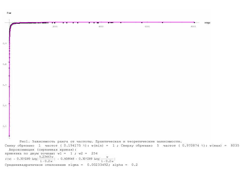
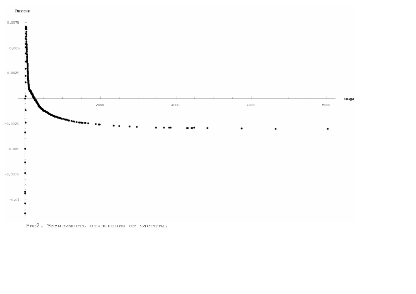
Figure 1: Top pane: image “Computer graphics” (http://www.vetton.ru/walls/art/vetton_ru_705.jpg). Bottom pane, left: the rank-frequency relation [circles: data; magenta line: least-squares fit $r(\omega)=(0.7576911\pm 0.012489081)+(0.1535386\pm 0.007973972)\log(\omega/(1+0.2\omega))$, where coefficients are given with 95% confidence intervals], right: error of the rank-frequency relation.

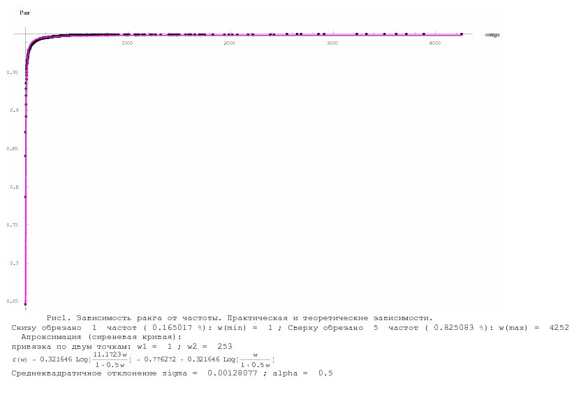
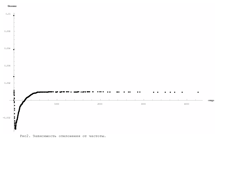
Figure 2: Top pane: image “A flower” (http://www.vetton.ru/walls/art/vetton_ru_175.jpg). Bottom pane, left: the rank-frequency relation [circles: data; magenta line: least-squares fit $r(\omega)=(0.87733668\pm 0.008050773)+(0.07762449\pm 0.005122996)\log(\omega/(1+0.2\omega))$, where coefficients are given with 95% confidence intervals], right: error of the rank-frequency relation.

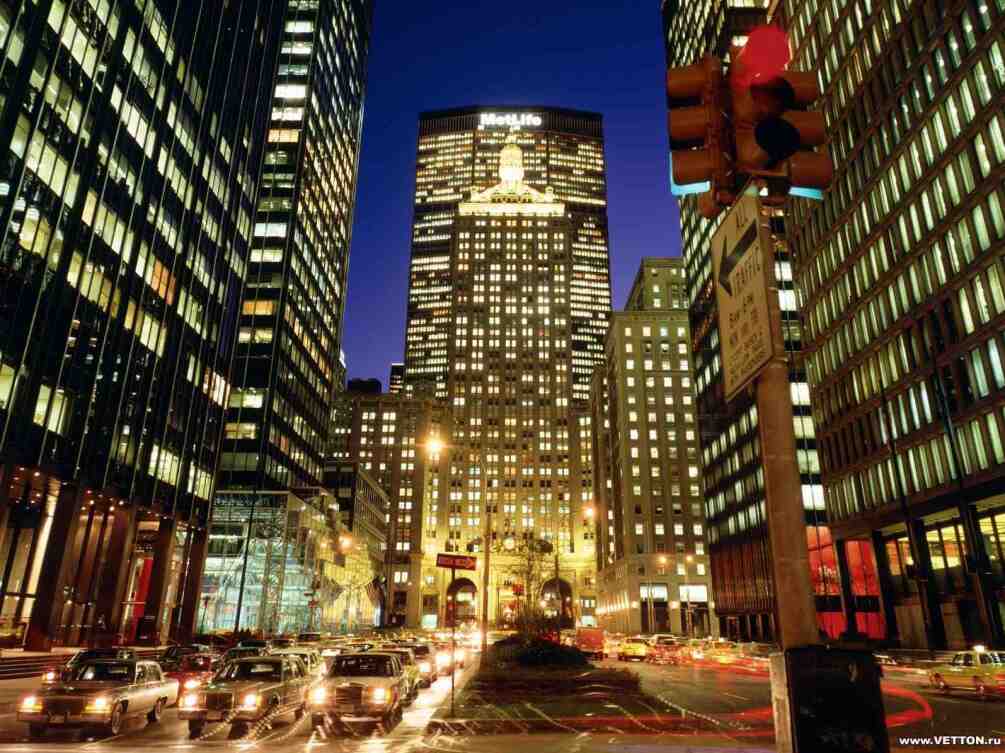
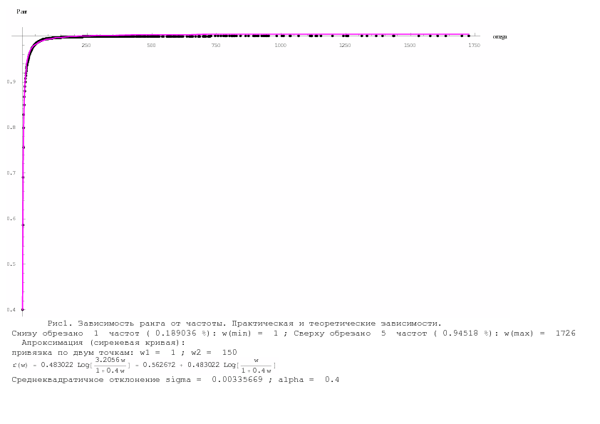
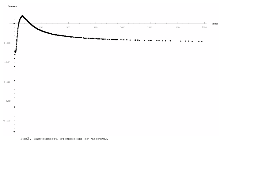
Figure 3: Top pane: image “New York by night” (http://www.vetton.ru/walls/art/vetton_ru_231.jpg). Bottom pane, left: the rank-frequency relation [circles: data; magenta line: least-squares fit $r(\omega)=(0.6807073\pm 0.01771724)+(0.2023832\pm 0.01130678)\log(\omega/(1+0.2\omega))$, where coefficients are given with 95% confidence intervals], right: error of the rank-frequency relation.

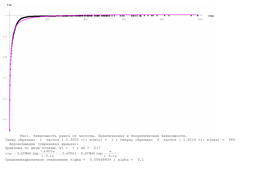
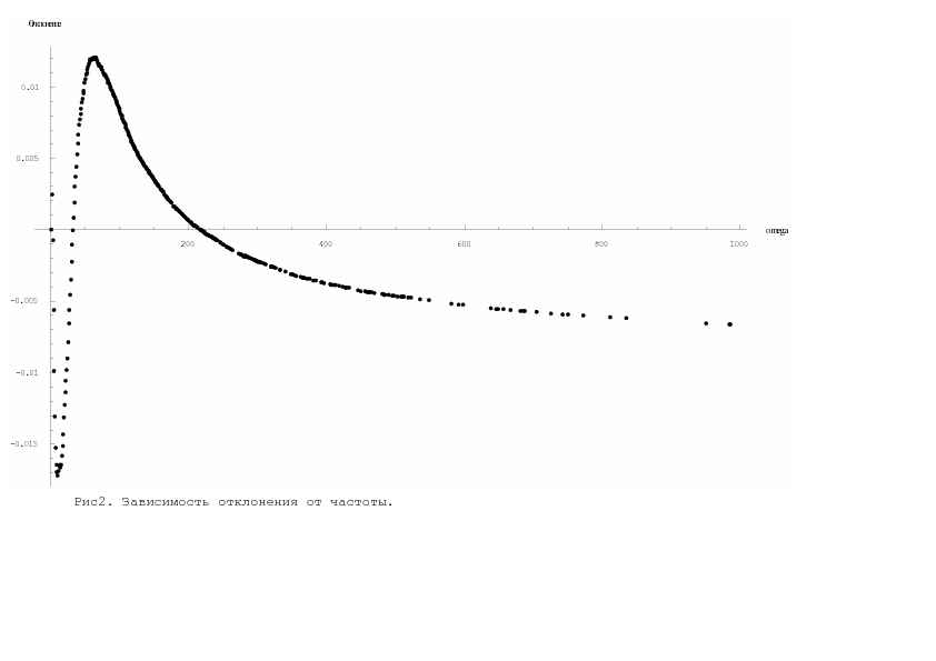
Figure 4: Top pane: image “The island.” Bottom pane, left: the rank-frequency relation [circles: data; magenta line: least-squares fit $r(\omega)=(0.7673719\pm 0.013762098)+(0.1483364\pm 0.008889888)\log(\omega/(1+0.2\omega))$, where coefficients are given with 95% confidence intervals], right: error of the rank-frequency relation.

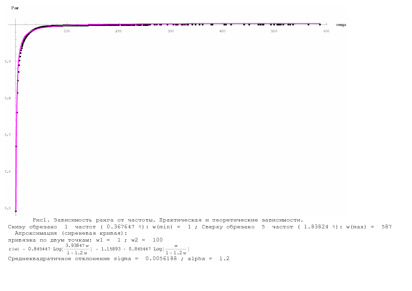
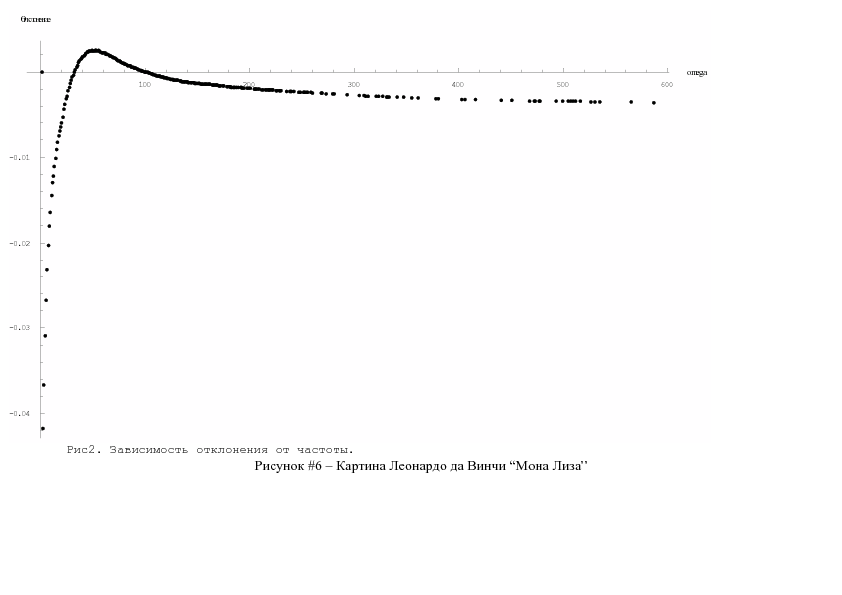
Figure 5: Top pane: image “The tiger” (http://www.vetton.ru/walls/art/vetton_ru_331.jpg). Bottom pane, left: the rank-frequency relation [circles: data; magenta line: least-squares fit $r(\omega)=(0.7555128\pm 0.01944519)+(0.1572145\pm 0.01265441)\log(\omega/(1+0.2\omega))$, where coefficients are given with 95% confidence intervals], right: error of the rank-frequency relation.

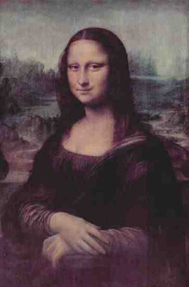
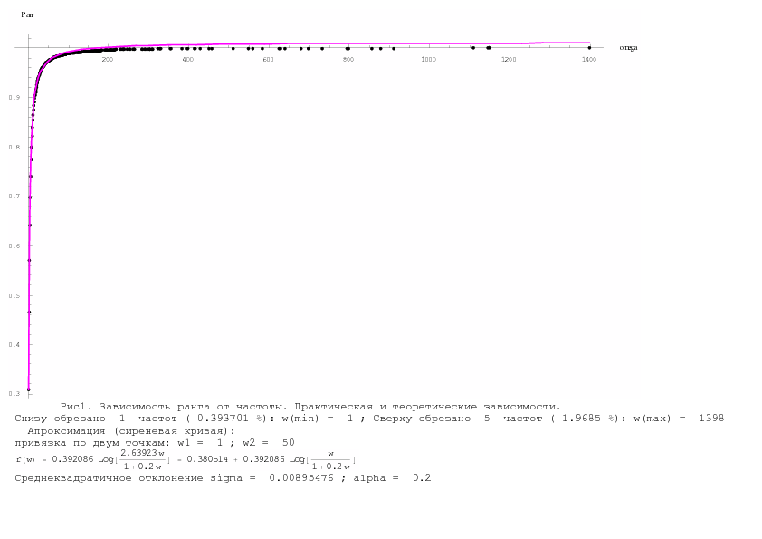
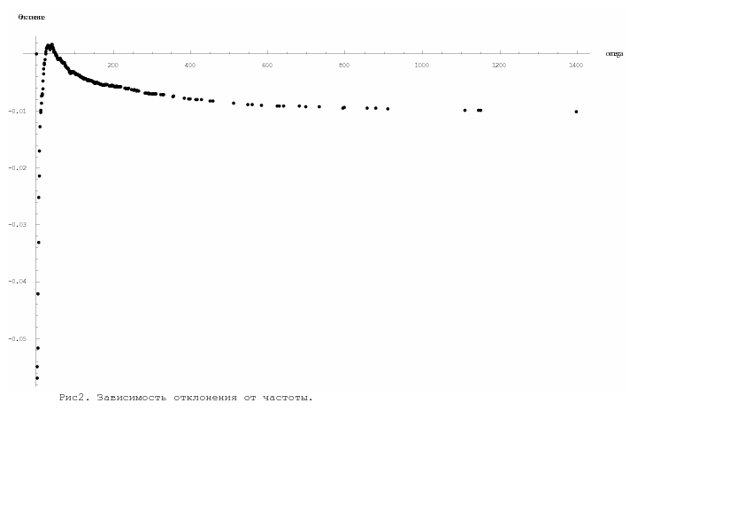
Figure 6: Top pane: image “Mona Liza.” Bottom pane, left: the rank-frequency relation [circles: data; magenta line: least-squares fit $r(\omega)=(0.5541642\pm 0.02411542)+(0.2860553\pm 0.01572469)\log(\omega/(1+0.2\omega))$, where coefficients are given with 95% confidence intervals], right: error of the rank-frequency relation.

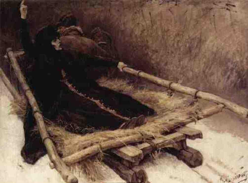
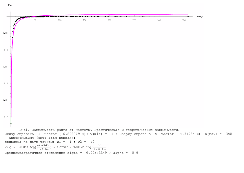
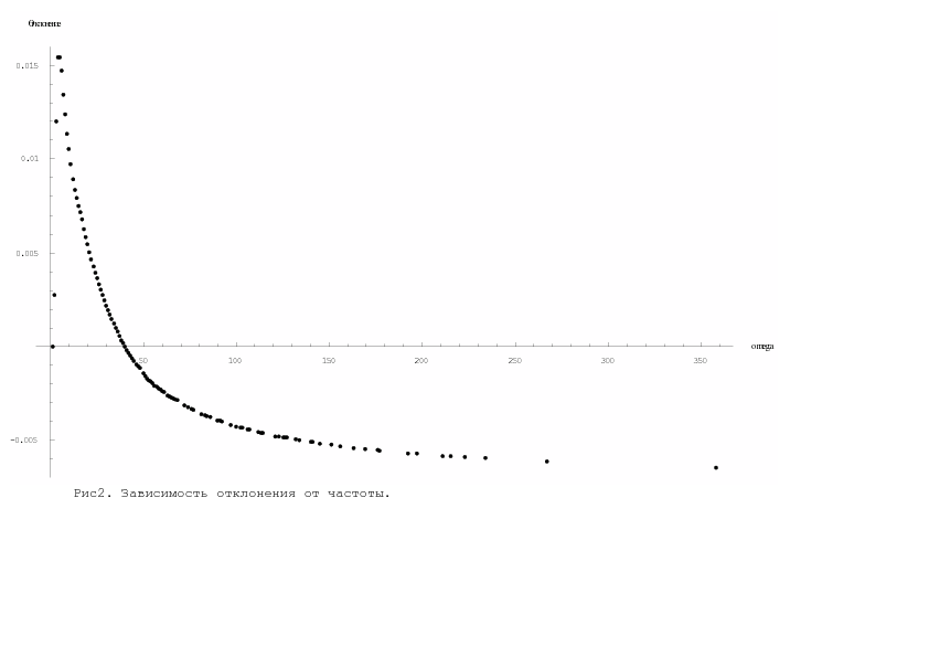
Figure 7: Top pane: image “Boyarynya Morozova.” Bottom pane, left: the rank-frequency relation [circles: data; magenta line: least-squares fit $r(\omega)=(0.85155937\pm 0.02285417)+(0.09873425\pm 0.01552277)\log(\omega/(1+0.2\omega))$, where coefficients are given with 95% confidence intervals], right: error of the rank-frequency relation.

The pictures were processed by N. Marchenko, who also learned how to “sew in” texts into pictures by steganographic methods. He took the color photograph of the tiger and “sewed into it” the text of Shakespeare’s King Richard the Third containing $190\,000$ symbols. The size of the file was not changed and the pictures of the tiger with or without King Richard were visually indistinguishable.

Further, one may find the dependence of the rank on the frequency for the modified picture with respect to the central line. To do this, one should take all pairs of points symmetric with respect to the central line, and then take the mean value of the colors $R=(R_{1}+R_{2})/2$, $G=(G_{1}+G_{2})/2$, $B=(B_{1}+B_{2})/2$ (thus in fact the upper half of the picture is rotated by 180 degrees in space and superimposed on the lower one). Then one may plot the dependence of rank on frequency as before.

After such a modification, the dictionary becomes $1.5$ times larger, and the maximal frequency decreases, and decreases significantly. This means that the picture has become much too gaudy (the distribution of colors has become more chaotic). The plot shows the degree of asymmetry. The inclusion of new objets must not breach this asymmetry.

9 Architecture. How to built within an existing ensemble

Synergetic studies show that human beings tend to acquire the opinions of the majority. It is known that the soldiers of the Russian army sent by the Commander-in-Chief to put an end to the February revolution in Saint Petersburg in 1917 were immediately imbued with the revolutionary spirit and took the side of the rebels.

G. Haken stressed the importance of a phenomenon which in physics led to the creation of laser emission. One of the authors of the present paper discovered, already in 1958, a remarkable phenomenon. If one slightly bends the parallel infinite mirrors in a laser, then a single mode laser emission occurs: the rays will not run away to infinity by diffraction, but will remain inside the infinite plate. Thus, from a chaotic bundle of rays in the open laser, a monochromatic wave is created, it remains within the open resonator, increases and, instead of diffusing according to the properties of waves all along the resonator, it remains in its “finite” part.

At the time it was impossible to construct such a monochromatic wave in narrow reflecting surfaces. At present this can probably be achieved by means of nanotechnologies.

Such a resonance phenomenon in human society and nature is still unexplained as a phase transition of the zeroth kind and requires additional study. It may be related to the sharpening regimes which S. P. Kurdyumov correlates with synergy problems.

However, it appears that the instrument best suited for falling into resonance is actually the human being. The spectator laughs or cries watching a film. Hostages are contaminated by the ideology of the terrorists that keep them in captivity (the Brussels syndrome). How people progressively become rhinoceroses (meaning fascists), even when they are least likely to be influenced by nazi ideology, is brilliantly shown by Ionesco in his play The Rhinoceroses. But if arians were easily converted to this ideology, nonarians were unable to become arians and therefore fascism was doomed from the outset.

The situation is quite different when invaders impose their religion and converting to it suffices not only to survive but to acquire equal rights. In that case, the newly converted sometimes become more fanatically zealous in their religion than the invaders.

B. F. Porshnev put forward the following paradoxal point of view on the appearance and development of mankind. Men at first were parasites attracted to the carnivores, like Maugli, and easily got used to their food and their voices. And while the wolf cub’s voice would change as it grew up, and it was rejected by its mother, a human could continue to produce the same sounds, and the she-wolf (or she-lion or other carnivore) would continue feeding the human. This easy adaptation to different kinds of foods, to different languages is characteristic of humans.

This point of view contradicts the usual one, according to which mankind created domestic animals. But from Porshnev’s point of view, humans first were the parasites of animals which they subsequently enslaved, as sometimes happens with people in everyday life.

In nature, the self-organization of animals takes place slowly, except perhaps during catastrophes. For people, we have the expression “become part of a collective,” “part of a team.” Humans become part of nature, which organizes itself. This determines the ultimate harmony and beauty of nature. Humans relax simply by observing it.

In the same way, ancient cities with their specific architecture fit in, blend into the surrounding landscape. This feeling increases if the observer is familiar with the history of the city. For example, after visiting York in England, a person becomes ready to feel the Shakespearian plays related to the period of the War of the Roses. The observer enters the atmosphere of the Middle Ages and is involuntarily penetrated by its spirit. Here everything is clear.

But if, inside an already existing ensemble of a city, a new architectural construction is added, how can one make it blend into the environment, self-organize itself into it, resonate with it? Clearly the surrounding nature and the already existing architectural ensemble will not adapt to the new construction (will not self-organize itself together with the new construction).

We know that Le Corbusier proposed to tear down Paris completely and replace it by new buildings from his projects.

Of course, we have the option of changing the ensemble or the surrounding landscape, but nature by itself will not resonate.

How could one verify if the Eiffel tower would blend into the old Paris? Did the glass pyramids blend with the Louvre? The answer is — yes, they did. Did the Kremlin Palace blend into the Kremlin ensemble? The Rossiya Hotel? One can photograph the ensemble and study the plots corresponding to the photographs with or without the palace; how will the “self-organization” plots change?

In our opinion, it is precisely this objective criterion which must determine whether or not a new building spoils the ensemble into which it is enclosed.

Whether or not such an addition enhances the effect of the ensemble is another question, it depends on the talent of the architect. But the objective verification of how it blends into the self-organized harmony is, of course, useful.

We used this approach when we carried out a practical experiment in the construction of out-of-town cottages. The houses were constructed in a forest, and our aim was to blend the structures into the “ensemble” of the forest, without touching it (Fig. 8 on p. 8). This involved, first, making apertures for the roots of the surrounding trees (the construction machines did not touch the trees). Secondly, we photographed the structures only from the sides that were visible through the forest. Thirdly, we took the photographs at different hours of the day (like Claude Monet, who painted the same bales of hay at different hours) and at different times of the year. Thus we obtained, as in the analysis of Quiet Flows the Don, a sufficiently wide spectrum of values for the parameters $\beta$ and $\sigma$.

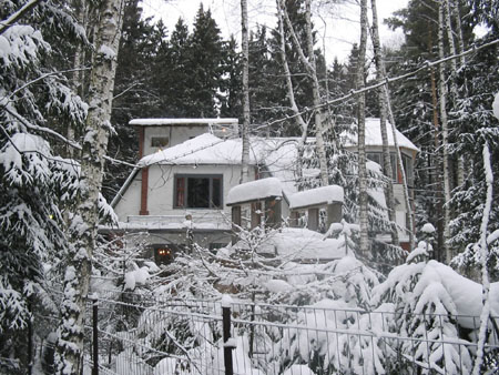
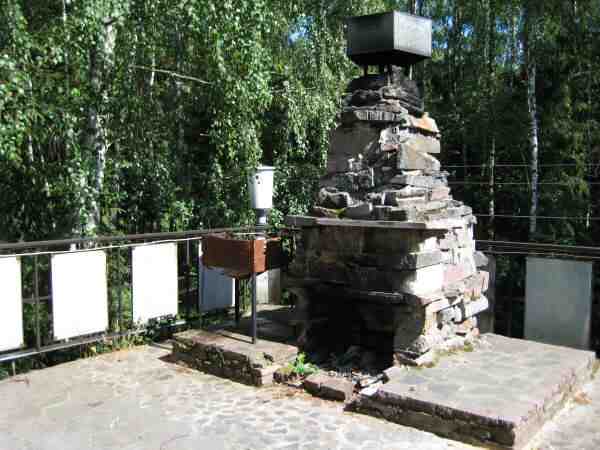
Figure 8: Images of a forest cottage.

Therefore, from the point of view of steganography, this need not be much of a problem. However, from the viewpoint of architecture, since one can never look at a building as a whole, since it is visible only from the open sides, this is a complicated approach. It is not surprising that in an article in the newspaper “Culture” (formerly “Soviet Culture”) describing one of the cottages, entitled “Windows of freedom and growth,” the title was followed by the subtitle “Academician Maslov broke all the rules of architecture, and not in vain.”

The computer allows to construct and study the picture before the object is constructed and photographed. Experimenting with a computer, we often remembered the words of Picasso: “I search — and I find.” But this is not enough. In our practice, it turned out that it was sometimes necessary to break down parts of the constructions already made.

At the present time, numerous cottages have been constructed near Moscow — this is a trait of our times. Many years ago, when the scientific town of Akademgorodok was being constructed near Novosibirsk, academicians Lavrentiev, Sobolev, and Khristianovich personally headed the construction and succeeded in saving a part of the forest in the middle of the new town. For the creative processes of research scientists, this was very important. It was also important for the teaching staff: after a lecture, a professor would walk through the forest and get rid of the “inspiration” needed to lecture, would relax. When one of the construction workers chopped down a small fir tree for Christmas, Lavretiev immediately threw him out of the city.

The forest has the same beneficial effect on composers, writers, and stage directors. A businessman or a political figure, returning to his out of town house after a hard day, can get rid of the stress, change air and atmosphere, modify the style of his office.

At the present, special computer software is used in the design and construction of new buildings. But this is not enough. The construction must fit into the “collective.” At the same time, the construction should be sufficiently modern, may even be close to the high tech style.

In our own practical construction, we were forced to modify the already constructed object, because we saw the drawbacks of the software that we used. It is necessary to correct “architectural” software so as to avoid such expensive mistakes.

The well-known architect F.Hundertwasser wrote: “People think that a building is its walls, but actually — it’s the windows.

Hundertwasser’s remark about windows is very relevant to our times. A person inside a house must feel like someone in a bathiscape in the underwater world. He must see and feel the exterior ensemble even when he is taking a shower.

But it is hard to agree with Hundertwasser when he claims that there are no straight lines in nature, and hence they should not appear in architecture. In nature, even in a mixed forest, straight lines do appear: light rays, falling through the leaves and producing shadows (compare, in painting, with the luchism theory of M. Larionov). Symmetry also appears, albeit not too strict: reflections in water, the inner symmetry of flowers, leaves, living organisms. There is also the fractal structure of snowflakes. All this must be reflected in the architecture of buildings that are to fit in the ensembles of nature.

To such a complex approach, one can apply the mathematical notion of “complexity”: it is inherent to nature, and it must be applied in architecture.Thus, the architecture of buildings in a cone forest, in which fir trees stand like “a shot from a rifle,” must differ from that in a mixed forest.

The relationship between mathematics and architecture has been noted long ago, especially in the architectural masterpieces of antiquity. Besides obeying the golden section rule, Greek temples blend harmoniously with the surrounding nature: the rocky slopes of the Acropolis in Athens, the Poseidon temple in Peloponnesus. Especially when they are open to the sea, when the mathematical harmony and rigor, the geometry of the doric columns, involuntarily bring to mind the name of Archimedes.

Architectural geometry is especially expressive with the background of a desert, as in the Sahara, where the Roman city of Sbaitl is situated.

In Istanbul, in Kairuan, in muslim cities with their tradition of covering the body and faces of women by clothing, this geometry has no limits. It is not surprising that the mosques of Istanbul, built on the basis of ancient temples, columns were turned upside down, with the capitols at ground level.

In Samarkand, we see a different kind of beauty, another geometry — the beauty of fractals. In Mexico architecture is related to rocks.

The relationship to rocks is also visible in gothic architecture, especially in certain castles. Here the geometry is also clearly expressed.

Sayings about semiotics in art (see [31]), relate especially well to architecture, where it is possible to identify and distinguish a set of signs.

In our approach, we look at the problem from a different angle, when the architectural signs in a complex structure are numerous and the structure is placed inside a very complex ensemble, and therefore the risk of destroying the harmony given to us by nature is high. It suffices to drive through some of the ugly settlements near Moscow to appreciate how serious the problem is. Or to visit the unique vacation center “Krainka” in the Tula region, where a magnificent old park, with trees situated so that their fallen leaves form a beautiful rug in autumn, is “embellished” by sculptures of half-naked javelin throwers. It suffices to photograph these “sculptures,” then delete them from the photograph, and compare the corresponding plots to see that these sculptures are incompatible with the harmony of the park. If we take a hammer and, following Rodin, remove all which is not needed, we may be left with little pieces of stone that will fit into the park. M. Voloshin used to repeat that a sculpture only acquires its final form after it is thrown down from a mountain.

Finally, a last general remark about architecture. No one today seriously considers adding arms to the Venus de Milo or restoring the missing pieces of the Perham altar. But in Russia many think that one can take an architectural structure and move it away from the place where it was constructed (as this was done in Suzdal), paint something over, renovate something, give the cupolas a shine. We propose, if such actions be undertaken, to first check the result by means of computations similar to those described in the present paper.

Returning to architecture in the forest, note that the structure of a house in the forest must be such that one will never tire of it, never be satiated with it. Your house has to be like a drug. The desire to return there must be like the nostalgia for one’s birthplace. You must feel attracted to your house, so that when you come in and light the chimney, you can sigh and say: finally, I am at home.

A house in the forest must not have any distances. You are in the forest. You have forgotten about the tedium of everyday life. Having plunged into this communion with nature for only a half hour, you should be able to get rid of the weight of your problems.

Different illuminations of the house, like different stage sets, must correspond to the mood that you want your close ones and yourself to feel. Thus, in Pitoev’s theater in Paris, at a certain time, the change of stage settings was replaced by changes in illumination. The illumination of the house, when you stand in the backyard, must be transparent, enhancing the beauty of the forest, so that you will want to cry out — “how beautiful!” And that is what architecture in a forest is about.

One can readily see that an asphalt road passing through a forest is a discord. Even in parks (e.g., in Versailles) the paths should not be covered by concrete. And all the more, if we want to preserve the heavenly chaos of a wild mixed forest. Cobblestones and gravel cost a lot more than asphalt, but the health of people related with what they see and smell is worth a lot more.

The beauty of “the fractal” is very well described by the outstanding Russian painter and graphic artist M. V. Dobuzhinsky, who really knew how to find sharp vantage points for his drawings of architectural fractals, viewpoints from which he obtained remarkable combinations of roofs, walls, columns, and other structures, briefly, of parts of an ensemble. In his “Recollections” he wrote: “All this I had already seen as a child on maps …and I started looking even more attentively at various geographic lines and silhouettes, noticing their remarkable elegance and, so to speak, of their organic structure. I was also very fond of finding unexpected repetitions of certain shore lines and contours of land, seas, lakes, and bays …I was also surprised by the repetition of some geographic outlines (e.g., the Peloponnes and the Galipoli trident, the Dutch Zeedersee and the Caspian bay of Karabogas, similar sand spits of Memel in the Baltic and Kinburn in Crimea)” [32], p. 99. It is well known that shorelines are fractals. The relationship between fractals and the formulas obtained above is characterized in [13]. The beauty of asymmetry, of divine chaos, of self-organizing chaos, obeying explicit laws, must be underlined, additionally stressed by the geometry of the added architectural structure, by the illumination. At least this should be attempted. As to the mathematical formulas, they can only show that we have not destroyed the already existing harmony.

The authors would like to express their gratitude to A. Churkin and N. Marchenko for help in computer calculations.

References

- [1] V. P. Maslov and T. V. Maslova, “Synergetics and Architecture,” Russ. J. Math. Phys. 15 (1), 102–121 (2008)
- [2] A. N. Kolmogorov, Collected Works in Mathematics and Mechanics (1985), pp. 136–137
- [3] V. P. Maslov, “Nonlinear Mean in Economics,” Mat. Zametki 78 (3), 377–395 (2005) [Math. Notes 78, 807–813 (2005)]
-
[4]
O. Viro, Dequantization of Real Algebraic
Geometry on Logarithmic. Texts for Students (2001);
http://www.pdmi.ras.ru/ olegviro/dequant - [5] M. van Manen and D. Siersma, “Power Diagrams and Their Applications,” arXiv:math/05058037, Aug 2, 2005
- [6] D. Alessandrini, “Logarithmic Limit Sets of Real Semi-Algebraic Sets,” arXiv:0707.0845 [math.AG] v1 5 Jul 2007
- [7] P. Maslov, “Phase Transitions of the Zeroth Kind,” Mat. Zametki 76 (5), 749–761 (2004)
- [8] V. P. Maslov, “Quasistable Economics and Its Relationship with the Thermodynamics of Superfluid Liquids. Default as a Phase Transition of Zeroth Kind. I” Review of Applied and Industrial Mathematics, Section “Mathematical Methods in Economics” 11 (11), 630–732 (2004); II 12 (1), 3–40 (2005)
- [9] G. Haken, “Self-Organizing Society,” in The Future of Russia in the Mirror of Synergetics (KomKniga, Moscow, 2006), pp. 194–208
- [10] C. Maincer, “Complexity Challenges Us in the 21st Century: Dynamics and Self-Organization in the Age of Globalization” in The Future of Russia in the Mirror of Synergetics (KomKniga, Moscow, 2006), pp. 209–226
- [11] V. P. Maslov, “Expertise and Experiment,” Novy Mir 1, 243–252 (1991)
- [12] V. P. Maslov, Quantum Economics (Nauka, Moscow, 2006) [in Russian]
- [13] V. P. Maslov, “Revision of Probability Theory from the Point of View of Quantum Statistics,” Russ. J. Math. Phys. 14 (1), 66–95 (2007)
- [14] V. P. Maslov, “The Lack-of-Preference Law and the Corresponding Distributions in Frequency Probability Theory,” Mat. Zametki 80 (2), 220–230 (2006) [Math. Notes 80, 214–223 (2006)]
- [15] V. P. Maslov, “On the Principle of Increasing Complexity in Portfolio Formation on the Stock Exchange,” Dokl. Acad. Nauk 404 (4), (2005) [Doklady Mathematics 72 (2), 718–722 (2005)]
- [16] L. D. Landau and E. M. Lifshits, Statistical Physics (Nauka, Moscow, 1976)
- [17] V. V. Vyugin and V. P. Maslov, “On Extremal Relations between Additive Loss Functions and Kolmogorov Complexity,” Probl. Inf. Transm. 39 (4), 71–87 (2003)
- [18] A. V. Podlasov, “The Theory of Self-Organizing Criticality as the Science of Complexity,” in The Future of Applied Mathematics. Lectures for Young Researchers, Ed. by G. G. Malinetskii (Editorial URSS, Moscow, 2005), pp. 404–426
- [19] A. T. Fomenko and T. G. Fomenko, “An Invariant of Authors of Russian Literary Texts,” in Methods of Quantitative Analysis of Texts from Narrative Sources (USSR Academy of Sciences, Institute of the History of the USSR, Moscow, 1983), pp. 86–109
- [20] V. P. Maslov and T. V. Maslova, “On the Zipf Law and Rank Distributions in Linguistics and Semiotics,” Mat. Zametki 80 (5), 718–732 (2006) [Math. Notes 80, 806–813 (2006)]
- [21] T. V. Maslova, “On the Specification of Zipf’s Law for Frequency Dictionaries,” NTI, Series 2, no. 11, 37–44 (2006)
- [22] B. Mandelbrot, The Fractal Geometry of Nature (Istitute of Computer Studies, Moscow, 2002) [in Russian]
- [23] M. V. Arapov, E. N. Efimova, and Yu. A. Shreider, “On the Meaning of Tank Distributions,” NTI, Series 2, no. 2, 9–20 (1975)
- [24] British National Corpus, ftp.itri.bton.ac.uk/pub/bnc
- [25] Mathematical Encyclopedic Dictionary (Moscow, 1988)
- [26] B. M. Malyutov, “Survey of Methods and Examples of the Attribution of Texts,” Review of Applied and Industrial Mathematics 12 (1), 41–77 (2005)
- [27] V. P. Maslov, “Quantum Linguistic Statistics,” Russ. J. Math. Phys. 13 (3), 315–325 (2006)
- [28] V. P. Maslov, “Negative Dimension in General and Asymptotic Topology,” arXiv:math.GM/0612543, Dec 19, 2006
- [29] V. P. Maslov, “Dimension of Holes and High-Temperature Condensate in Bose-Einstein Statistics,” arXiv:physics/0612182, Dec 22, 2006
- [30] V. P. Maslov, “Secondary Dequantization in Algebraic and Tpopical Qeometry,” Mat. Zametki 82 (6), 953–954 (2007) [Math. Notes 82, 860–862 (2007)]
- [31] V. V. Ivanov, Essays on the History of Semiotics in the USSR (Nauka, Moscow, 1976) [in Russian]
- [32] M. V. Dobuzhinsky, Recollections (Nauka, Moscow, 1987) [in Russian]