X-ray hiccups from Sgr A* observed by XMM-Newton

Abstract

Context. Our Galaxy hosts at its dynamical center Sgr A*, the closest supermassive black hole. Surprisingly, its luminosity is several orders of magnitude lower than the Eddington luminosity. However, the recent observations of occasional rapid X-ray flares from Sgr A* provide constraints on the accretion and radiation mechanisms at work close to its event horizon.

Aims. Our aim is to investigate the flaring activity of Sgr A* and to constrain the physical properties of the X-ray flares.

Methods. In Spring 2007, we observed Sgr A* with XMM-Newton with a total exposure of $\sim$230 ks. We have performed timing and spectral analysis of the new X-ray flares detected during this campaign. To study the range of flare spectral properties, in a consistent manner, we have also reprocessed, using the same analysis procedure and the latest calibration, archived XMM-Newton data of previously reported rapid flares. The dust scattering was taken into account during the spectral fitting. We also used Chandra archived observations of the quiescent state of Sgr A* for comparison.

Results. On April 4, 2007, we observed for the first time within a time interval of roughly half a day, an enhanced incidence rate of X-ray flaring, with a bright flare followed by three flares of more moderate amplitude. The former event represents the second brightest X-ray flare from Sgr A* on record. This new bright flare exhibits similar light-curve shape (nearly symmetrical), duration ($\sim$3 ks) and spectral characteristics to the very bright flare observed in October 3, 2002 by XMM-Newton. The measured spectral parameters of the new bright flare, assuming an absorbed power law model taken into account dust scattering effect, are $N_{\rm H}$=12.3${}^{+2.1}_{-1.8}\times 10^{22}$ cm^-2 and $\Gamma\sim$2.3$\pm$0.3 calculated at the 90% confidence level. The spectral parameter fits of the sum of the three following moderate flares, while lower ($N_{\rm H}$=8.8${}^{+4.4}_{-3.2}\times 10^{22}$ cm^-2 and $\Gamma\sim$1.7${}^{+0.7}_{-0.6}$), are compatible within the error bars with those of the bright flares. The column density found, for a power-law model taking into account the dust scattering, during the flares is at least two times higher than the value expected from the (dust) visual extinction toward Sgr A* ($A_{\rm V}\sim 25$ mag), i.e., 4.5$\times 10^{22}$ cm^-2. However, our fitting of the Sgr A* quiescent spectra obtained with Chandra, for a power-law model taking into account the dust scattering, shows that an excess of column density is already present during the non-flaring phase.

Conclusions. The two brightest X-ray flares observed so far from Sgr A* exhibited similar soft spectra.

1 Introduction

Located at the center of our Galaxy, Sgr A* is the closest supermassive black hole to the solar system at a distance of about 8 kpc (Reid 1993; Eisenhauer et al. 2003, 2005). Its mass of about 3–4$\times$10⁶ $M_{\odot}$ has been determined thanks to the measurements of star motions (e.g., Schödel et al. 2002; Ghez et al. 2003, 2005). Amazingly, this source is much fainter than expected from accretion onto a supermassive black hole. Its bolometric luminosity is only about 3$\times$10^-9 L_Edd (Melia & Falcke 2001; Zhao et al. 2003). In particular, its 2–10 keV X-ray luminosity is only about 2.4$\times$10³³ erg s^-1 within a radius of 1.5^′′ (Baganoff et al. 2003). Thus, Sgr A* radiates in X-rays at about 11 orders of magnitude less than its corresponding Eddington luminosity. This has motivated the development of various radiatively inefficient accretion models to explain the dimness of the Galactic Center black hole, e.g., Advection-Dominated Accretion Flows (e.g., Narayan et al. 1998), jet-disk models (e.g., Falcke & Markoff 2000), Bondi-Hoyle with inner Keplerian flows (e.g., Melia et al. 2000). The recent discovery of X-ray flares from Sgr A* has provided new exciting perspectives for the understanding of the processes at work in the Galactic nucleus.

The first detection of such events was found with Chandra in October 2000. This flare had a duration of about 10 ks, with a flare peak luminosity of about 1.0 $\times$ 10³⁵ erg s^-1, in the 2–10 keV energy range, i.e., about 45 times the quiescent state (Baganoff et al. 2001). Further on several other X-ray flares were detected by XMM-Newton (Goldwurm et al. 2003; Porquet et al. 2003; Bélanger et al. 2005) and Chandra (Baganoff 2003; Eckart et al. 2004, 2006, 2008; Marrone et al. 2008). The majority of X-ray flares detected up to now have moderate flux amplitude with factor of about 10–45 compared to the quiescent state. Only one very bright flare with a flux amplitude of about 160 was observed in October 2002 (Porquet et al. 2003). Remarkably, its peak luminosity of $\sim$3.6$\times$10³⁵ erg s^-1 was comparable to the bolometric luminosity of Sgr A* during its quiescent state. The light curve of the X-ray flares can exhibit short (e.g., 600 s, Baganoff et al. 2001; 200 s, Porquet et al. 2003) but deep drops close to the flare maximum. This short-time scale could indicate that the X-ray emission is emitted from a region as small as 7$R_{\rm S}$ ($\sim$ 13 $R_{\odot}$).

In contrast to the near-IR (NIR) flares which appear to be present for up to 40% of the time (e.g., Genzel et al. 2003; Ghez et al. 2004; Yusef-Zadeh et al. 2006, Yusef-Zadeh et al. 2008 in prep.), the X-ray flaring has a much lower duty cycle, of typical 1-5% (Baganoff 2003; Bélanger et al. 2005; Eckart et al. 2006). This means either that the majority of NIR flares have no X-ray counterpart or that the X-ray-to-NIR ratio of some of the flares is too small to allow an X-ray detection above the strong, diffuse X-ray emission from the central parsec. When both NIR and X-ray flares are detected simultaneously, they show similar morphology in their light curves as well as no apparent delay between the peaks of flare emission (Eckart et al. 2004, 2006, 2008; Yusef-Zadeh et al. 2006). The current interpretation is that both flares come from the same region.

We report here the results of our Sgr A* observation campaign performed with XMM-Newton from March 30 to April 4, 2007. The whole results of this multi-wavelength campaign (VLA, CSO, VLT/NACO-VISIR, HST/NICMOS, Integral) will be reported elsewhere (Yusef-Zadeh et al. 2008 in prep.; Dodds-Eden et al. 2008, in prep.). We also observed during the three XMM-Newton observations, two bright transient sources in outburst (Porquet et al. 2007). The source located at about 90^′′–SW from Sgr A* has been associated with the eclipsing X-ray burster AX J1745.6-2901. Seven deep eclipses were observed as well as type-I bursts. The second source is located at about 10^′–NW from Sgr A* and has been associated with the neutron star low-mass X-ray binary GRS 1741.9-2853 (a.k.a. AX J1745.0-2855). The data analysis of these two sources will be reported in forthcoming papers.

We report, here, for the first time a high level of flaring activity with four X-ray flares, one bright and three moderate, detected in half a day. The bright flare is the second brightest X-ray flare detected so far from Sgr A*.

In $\S$2 we describe the observations and data reduction procedure used in this work. In $\S$3 we report the timing analysis of Sgr A*, and the spectral analysis of the bright flare and the sum of the three following moderate flares observed during this Spring 2007 campaign. In $\S$4, we perform a homogeneous and self-consistent comparison of spectral properties of the X-ray flares of this campaign with the reprocessed data of X-ray flares previously observed with XMM-Newton. Finally, in $\S$5 we summarize our main results and discuss their possible implications.

2 XMM-Newton observations and data reduction

We observed Sgr A* three times with XMM-Newton in Spring 2007 for a total exposure of $\sim$230 ks. The journal of the XMM-Newton observations is given in Table 1. The EPIC cameras, 2 MOS (Turner et al. 2001) and one pn (Strüder et al. 2001), were operated in the full frame window mode with the medium filter. We use the version 7.1 of the Science Analysis Software (SAS) package for the data reduction and analysis, with the latest release of the Current Calibration files (CCF). The MOS and pn event lists were produced using the SAS tasks emchain and epchain. The detector light curves in the 7–15 keV energy range computed by these tasks show that the levels of background proton flares were high only during the last seven hours of the second and the third observations, where the count rate exceeded the detector telemetry limit, triggering the counting mode.

For the timing analysis, the contribution of the background proton flares was estimated using a $\sim$$3\arcmin\times 3\arcmin$ area with a low level of X-ray extended-emission, located at $\sim 4\arcmin$-North of Sgr A* on the same CCD, where the X-ray emission of point sources were subtracted.

Table 1: XMM-Newton observation log for the Spring 2007 campaign.

Orbit	ObsID	Start time	End time	duration
		(UT)	(UT)	(ks)
1338	402430701	Mar 30, 21:29:18.1	Mar 31, 06:28:20.8	32.3
1339	402430301	Apr 1, 15:09:03.5	Apr 2, 19:54:45.8	103.5
1340	402430401	Apr 3, 16:40:21.5	Apr 4, 19:47:39.2	97.6

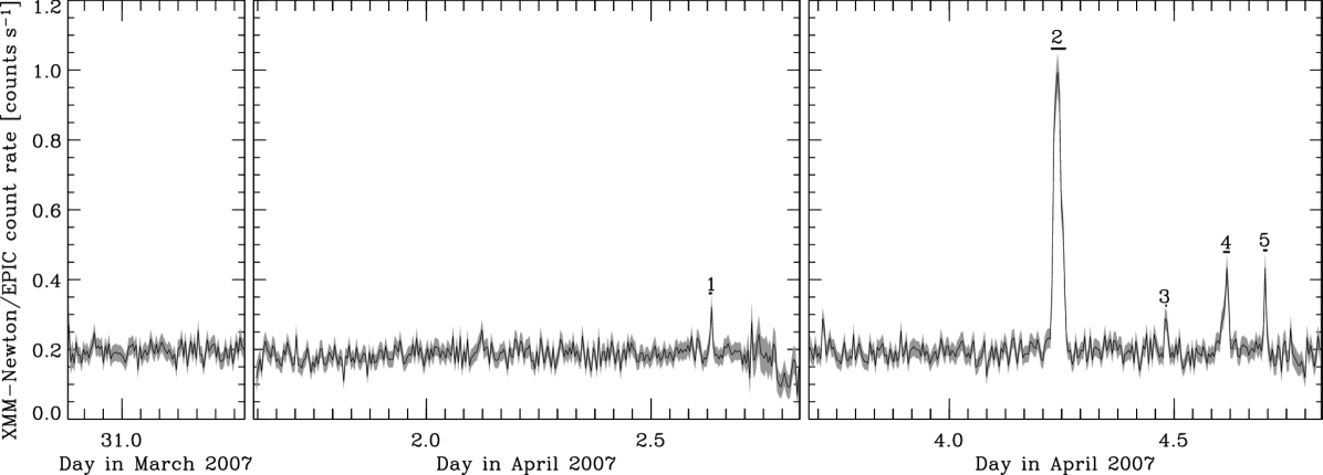
Figure 1: XMM-Newton/EPIC (pn+MOS1+MOS2) light curves of Sgr A* in the 2–10 keV energy range obtained in Spring 2007. The light curves are corrected from soft-proton flaring background. The time interval used to bin the light curve is 350 s. The X-ray flares are labeled from 1 to 5. The horizontal lines below these labels indicate the flare durations. The quiescent level of Sgr A* corresponds to only 10% of the non-flaring level of these light curves (see text for details).

.

To optimize in our three observations the selection of the events from Sgr A*, we used a two-step method based on the flaring activity of Sgr A* and the presence of the two bright transient sources. We first computed for each observation a sky image in the 2–10 keV energy range that was used to define a circular region of 10$\arcsec$-radius centered on the X-ray source associated with Sgr A*. From this extraction region, we built a preliminary background-subtracted light curve to identify any flare from Sgr A*. We identified a bright flare from this extraction region in the last observation. Its position in each detector was determined with the SAS task edetect_chain using only the flare time interval, while the positions of the other X-ray sources were determined using the whole exposure of the last observation. The angular distances between the flaring X-ray source associated with Sgr A* and the two bright transient sources (e.g., for pn $87.5\arcsec\pm 0.2\arcsec$ and $599.9\arcsec\pm 0.2\arcsec$, respectively) were then used to determine the relative position of Sgr A* in the two other observations. This method is independent to any variation of the detector position angle. Then, we use the X-ray counterparts of the Tycho-2 catalog’s sources (Høg et al. 2000) to obtain an absolute astrometry (see Appendix A for details). The absolute position of the X-ray bright flare is $\alpha_{\rm J2000}=17^{\rm h}45^{\rm m}40.0^{\rm s}$, $\delta_{\rm J2000}=-29^{\circ}00^{\prime}28.6\arcsec$ with a one-sigma positional uncertainty of $1\aas@@fstack{\prime\prime}0$, i.e., only $0\aas@@fstack{\prime\prime}5$ from the radio position of Sgr A* (Yusef-Zadeh et al. 1999). Therefore, the position of the X-ray bright flare is fully consistent with the radio position of Sgr A*.

3 Results

3.1 X-ray light curves of Sgr A*

For each observation and detector, we first built the source+background and the background light curves in the 2–10 keV energy range with 1 s time bins starting (stopping) at the first (last) good time interval (GTI) of the corresponding CCD. We rebinned the light curves to 350 s to increase the S/N. Then, we subtracted the background light curve (scaled to the same source extraction area) from the source+background light curve. We scaled up, using GTI information, count rates and errors affected by the lost of exposure (e.g., due to the switch from science to counting mode).

Finally, the background-subtracted light curves of the three detectors were summed to produce the EPIC light curves. Any detector missing value was inferred by the one observed by the other detectors using a (median) scaling factor between the detectors.

The EPIC (pn+MOS1+MOS2) background subtracted light curves of Sgr A* in the 2–10 keV energy range, with a time bin interval of 350 s, are shown in Fig. 1. During the first half of the exposure, the light curve is almost flat, with a non-flaring level of X-ray emission consistent with the one observed with XMM-Newton in 2000 (Goldwurm et al. 2003) and 2002 (Porquet et al. 2003). The $\sim$50% higher non-flaring level observed in 2004 with XMM-Newton (Bélanger et al. 2005) was due to the contamination by a close transient source in outburst (Muno et al. 2005; Porquet et al. 2005), see also $\S$4. Excluding Sgr A* and any transient sources in outburst, the X-ray emission inside the $10\arcsec$-radius region centered on Sgr A* comes mainly from one point source associated with the complex of stars IRS 13, the candidate pulsar wind nebula G359.95-0.04, and a diffuse component (Baganoff et al. 2003; Muno et al. 2003; Wang et al. 2006), which contribute to about 90% of the non-flaring level in the 2–10 keV energy range.

We identify any significant deviation from the non-flaring level as possible flare. A possible ($\#1$) was observed on April 2, 2007. On April 4, one bright flare ($\#2$) was observed followed by three moderate flares ($\#3$, $\#4$, and $\#5$). Figures 2 and 3 focus on the flare light curves with a bin time interval of 100 s that we use to characterize these flares. We use an iterative sigma-clipping of the light curve of each observation to compute the mean non-flaring level (dashed line) and its standard deviation. We define the flare time interval as the period where the light curve deviates from the mean non-flaring level at a confidence level of 95% (i.e., where the light curve is above its mean non-flaring level plus 1.64 times its standard deviation). Table 2 gives the characteristics of these X-ray flares. The weak flare $\#1$ peaks just above 3 sigma, and it is, therefore, considered as reliable. This weak flare was independently confirmed by a simultaneous detection in IR by HST/NICMOS (Yusef-Zadeh at al. 2008, in preparation).

The bright flare has a duration of about 3 ks, similar to the duration that was observed for the (brightest) flare of October 2002 (Porquet et al. 2003). Its light curve is almost symmetrical, but no significant deep drop (i.e., about 50% of flux decrease) is observed in contrast to the flares of September 2000 (Baganoff et al. 2003) and October 2002 (Porquet et al. 2003). Indeed, in the case of the October 2002 flare, the significant drop was observed in all three instrument light curves, while the apparent drop in the EPIC light curves of flare $\#$2 is only observed in the pn light curve. However, for the flare $\#$2 we cannot rule out a moderate drop in the X-ray light curve. We also computed the hardness ratio using the 2–5 keV and 5–10 keV energy ranges, but we found no significant spectral change during the flare interval.

The peak count rates of the moderate flares are 2–6 smaller than that of the bright flare. The durations of the moderate flares are 2–10 times shorter than of the bright one. The time gaps between two consecutive flares starting from flare $\#$2 are 5.3, 3.0 and 1.8 hours. Therefore, four flares were observed in a time interval of only half a day. A similar group of three moderate flares were already observed with XMM-Newton on 2004 March 31 (Bélanger et al. 2005), but no such preceding bright flare was observed. This is the first time that a such level of X-ray flaring activity from Sgr A*, both in amplitude and frequency, is reported.

When the time coverage of the NIR observations allowed simultaneous observations with XMM-Newton, the NIR counterparts of these X-ray flares have been observed: flares $\#1$, $\#4$, and $\#5$ were observed with HST/NICMOS (Yusef-Zadeh et al. 2008, in prep.); and flare $\#2$ was observed with VLT/NACO (Dodds-Eden et al. 2008, in prep.).

Figure 2: XMM-Newton/EPIC light curve of the bright flare in the 2–10 keV energy range. The light curve is corrected from soft-proton flaring background. The bin time interval is 100 s. The dashed and dotted lines indicate the mean non-flaring level and the 1.64$\sigma$ threshold, respectively (see text for details). The dotted-dashed vertical lines indicate the time interval where the light curve deviates from its mean level at a confidence level of 95$\%$.

Figure 3: XMM-Newton/EPIC background-subtracted light curve of the moderate flares in the 2–10 keV energy range. Same definitions, and time duration, as in Fig. 2.

3.2 Spectral analysis of the X-ray flares

Table 2: Characteristics of the X-ray flares observed in April 2007 (see Fig.  2 and 3).

Flare	Day	Start time(a)		End time(a)		Duration	Total(b)	Peak(c)	Det.(d)	$L_{\rm 2-10\leavevmode\nobreak\ keV}^{\rm peak\leavevmode\nobreak\ (e)}$	Ampl.(f)
#		hh:mm:ss	s	hh:mm:ss	s	s	cts	cts s-1	$\sigma$	1034 erg s-1
1	2	15:05:03	291913503	15:15:03	291914103	600	50.9	0.160	3.1	3.3${}^{+1.2}_{-0.7}$	14${}^{+5}_{-3}$
2	4	05:25:30	292051530	06:13:50	292054430	2900	1443.0	1.052	20.6	24.6${}^{+4.8}_{-3.3}$	103${}^{+20}_{-14}$
3	4	11:32:10	292073530	11:37:10	292073830	300	60.4	0.291	5.7	6.1${}^{+2.2}_{-1.2}$	25${}^{+9}_{-5}$
4	4	14:37:10	292084630	14:58:50	292085930	1300	212.1	0.301	5.9	6.3${}^{+2.3}_{-1.3}$	26${}^{+9}_{-5}$
5	4	16:45:30	292092330	16:58:50	292093130	800	127.6	0.426	8.4	8.9${}^{+3.2}_{-1.8}$	37${}^{+13}_{-7}$

• Start and end times of the flare time interval defined as the period where the EPIC light curve deviates from the non-flaring level at a confidence of 95%. See text for details.

• Total EPIC counts in the 2–10 keV energy band obtained during the flare interval after subtraction of the non-flaring level.

• EPIC count rate in the 2–10 keV energy band at the flare peak after subtraction of the non-flaring level.

• Detection level at the flare peak in $\sigma$.

• 2–10 keV luminosity at the flare peak, assuming an absorbed power law model (taking account dust scatter effect), see parameter fits in Table 3.

• Amplitude of the flare defined as the ratio of the 2–10 keV flare luminosity at the peak and the 2–10 keV quiescent luminosity of Sgr A* observed with Chandra (i.e., 2.4 $\times$ 10³³ erg s^-1, Baganoff et al. 2003, and this work, see $\S$4).

We report here the spectral analysis of the four flares observed during the third observation. We used as extraction region for each instrument, a 10^′′-radius region centered on the position of Sgr A* determined during the bright flare time interval ($\S$2). The determination of the time interval of the X-ray flare is crucial to prevent from any bias in the spectral analysis. For example, in case the flare time interval includes a significant fraction of non-flaring level, we find that both column density and power-law slope values are bias. This is more important for moderate and weak flares. We selected X-ray events with FLAG equal to zero, and since pile-up was negligible, even during the bright flare, with patterns 0–12 and 0–4 (single and double) for the MOS and pn, respectively. To extract the background spectrum we used the same region but limited to the non-flaring time interval. The response matrices and ancillary files were computed using the SAS tasks rmfgen and arfgen, respectively. We used XSPEC (version 12.4.0; Arnaud 1996) to fit the spectrum with X-ray emission models. We report in Table 3 the spectral analysis of the bright flare $\#2$, and of the sum of the three following moderate flares (i.e., $\#3$+$\#4$+$\#5$) to increase the statistics. Instead of using the $\chi^{2}$ statistic, which is not appropriate for the fitting of spectra with low counts (e.g., $\#3+\#4+\#5$), we use a modified version of cstat statistic (Cash 1979) called the $W$ statistic (Wachter et al. 1979) that is implemented in XSPEC (Arnaud, in prep.). The $W$ statistic is valid for unbinned background-subtracted spectra. Binning would erase information and bias the fitting result. We show in online Appendix B that for rather bright flares (e.g., flare $\#2$) the parameter fits obtained using this $W$ statistic are very similar to that found using the $\chi^{2}$ statistic (Table 5); but the error bars obtained using the $W$ statistic are much better constrained. We fit the spectra in the 1–10 keV energy range. We would like to notice that similar parameter fits are found when fitting in the 0.3–10 keV and 2–10 keV energy ranges.

The column density ($N_{\rm H}$) of the gas along the line-of-sight absorbing the X-ray photons was fitted using the XSPEC model wabs (Morrison & McCammon 1983), which uses the (old) solar abundances of Anders & Ebihara (1982). We notice that significant revisions of the solar abundances have been made recently (see e.g., Asplund et al. 2005, for a review), leading to a decrease of the metal abundances, in particular of carbon and oxygen, which are the main contributors to the photoionization cross section above 0.3 and 0.6 keV. Therefore, using these revised solar abundances would increase the absolute derived value of column density by about 50% (Grosso et al. 2007), with a negligible impact on the derived value of the photon index. We also include the effect of the dust scattering, which deviates soft X-ray photons from our line-of-sight, using P. Predehl’s XSPEC scatter model (Predehl & Schmitt 1995). The scatter model multiplies the intrinsic spectrum by $\exp{(-\tau_{\rm sca})}$, where $\tau_{\rm sca}$ is the scattering optical depth, which is given by $\tau_{\rm sca}=0.087\times(A_{\rm V}/{\rm mag})\times(E/{\rm 1\,keV})^{-2}$ (Predehl & Schmitt 1995). From the $K$-band extinction value of 2.8$\pm$0.2 mag toward Sgr A* obtained using VLT/SINFONI (Eisenhauer et al. 2005) and the extinction law of Rieke & Lebofsky (1985), we inferred a dust visual extinction value of A_V= 25.0$\pm$1.8 mag.

Table 3: Best fit parameters (using $W$ statistic, see text for details) of the EPIC flare spectra for absorbed pegged power-law (pow), bremsstrahlung (brems), and black-body (bb) models, taking into account dust scattering (assuming A_v=25 mag). The errors are given at the 90% confidence level.

Flare	Model	$N_{\rm H}^{\rm\,(a)}$	$\Gamma$/kT(b)	$F_{2-10\,{\rm keV}}^{\rm mean\leavevmode\nobreak\ (c)}$	C/d.o.f.
April 2007
$\#2$	pow	12.3${}^{+2.1}_{-1.8}$	2.3${}^{+0.3}_{-0.3}$	16.1${}^{+3.1}_{-2.2}$	2560/2998
	brems	10.8${}^{+1.6}_{-1.4}$	6.9${}^{+3.1}_{-1.7}$	13.7${}^{+4.3}_{-2.9}$	2559/2998
	bb	6.6${}^{+1.3}_{-1.2}$	1.5${}^{+0.1}_{-0.1}$	9.7${}^{+0.7}_{-0.7}$	2562/2998
$\#3$+$\#4$+$\#5$	pow	8.8${}^{+4.4}_{-3.2}$	1.7${}^{+0.7}_{-0.6}$	5.0${}^{+1.8}_{-1.0}$	2117/2998
	brems	8.3${}^{+3.5}_{-2.4}$	$\geq$ 7.0	4.8${}^{+2.6}_{-0.8}$	2117/2998
	bb	4.3${}^{+2.8}_{-2.0}$	1.9${}^{+0.4}_{-0.3}$	3.6${}^{+0.7}_{-0.6}$	2117/2998
October 3, 2002
	pow	12.3${}^{+1.6}_{-1.5}$	2.2${}^{+0.3}_{-0.3}$	25.3${}^{+3.6}_{-2.7}$	2728/2998
	brems	10.7${}^{+1.2}_{-1.1}$	8.2${}^{+3.3}_{-1.9}$	21.9${}^{+5.2}_{-3.6}$	2729/2998
	bb	6.4${}^{+1.0}_{-0.9}$	1.6${}^{+0.1}_{-0.1}$	15.6${}^{+0.9}_{-0.8}$	2741/2998

• $N_{\rm H}$ is given in units of 10²² cm^-2.

• The black-body temperature is given in keV.

• Mean unabsorbed fluxes for the flare period in the 2–10 keV energy range in units of 10^-12 erg cm^-2 s^-1.

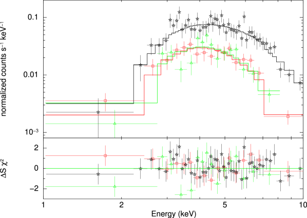
Figure 4: XMM-Newton EPIC spectra of the flare $\#2$ observed during the April 2007 observation campaign. The spectrum for the non-flaring period with the same extraction region is used as background. Squares, triangles and stars indicate MOS1 (red), MOS2 (green), and pn (black) data, respectively. The lines show the best-fit model using an absorbed power-law model taking into account dust scattering (see Table 5 for the best fit parameter values using $\chi^{2}$ statistic; pow model). The fit residuals are shown in the bottom panel.

We fitted the spectra in turn with the following continuum models: a pegged power-law model (pegpwrlw model in XSPEC), a bremsstrahlung model, and a black-body model. The parameters were tied between MOS1, MOS2, and pn spectra. Table 3 gives for these models the best fit parameters and errors at the 90% confidence level. The best-fit parameters of flare $\#2$ are rather well constrained for the three models. For the absorbed power-law model we found $N_{\rm H}$=12.3${}^{+2.1}_{-1.8}$$\times$ 10²² cm^-2 and $\Gamma$=2.3$\pm$0.3. As reported in Table 5, very similar best fit parameters are obtained using the $\chi{{}^{2}}$ statistic ($N_{\rm H}$=12.8${}^{+2.5}_{-2.1}$$\times$ 10²² cm^-2 and $\Gamma$=2.3$\pm$0.4). For illustration purpose, we report in Fig. 4 the corresponding background-subtracted binned EPIC spectra and the data/model fit residuals obtained using the $\chi{{}^{2}}$ statistic. The presence of a narrow Fe K${\alpha}$ Gaussian emission lines ($\sigma$=10 eV) is not statistically required ($\Delta\chi^{2}<$1 for one additional parameter). We find at 6.4 keV, 6.7 keV, and 7.0 keV upper limits on the equivalent widths of 154 eV, 135 eV, and 145 eV, respectively. We also test for spectral variation index during the flare. First, splitting the spectra into two equal parts (as done in Porquet et al. 2003), we obtained $N_{\rm H}$=13.0${}^{+2.9}_{-2.5}$$\times$ 10²² cm^-2, $\Gamma$=2.5${}^{+0.5}_{-0.4}$, and $N_{\rm H}$=11.6${}^{+3.0}_{-2.6}$$\times$ 10²² cm^-2, $\Gamma$=2.1$\pm$0.5, for the rising and decreasing phases, respectively. These values are consistent within the error bars. If we tied the values of the column density (i.e., if we assume that it is constant during the flare), we found $\Gamma$=2.4${}^{+0.4}_{-0.3}$ and $\Gamma$=2.2$\pm$0.4, for the rising and decreasing phases, respectively. Therefore, in both case, there is no significant (at a 90$\%$ confidence level) spectral variations during the flare, consistent with the lack of spectral variability inferred above from the hardness ratio. The same conclusion is found when splitting the spectra into three parts: rising, top, and decreasing phases. The flare $\#2$ data are also very well fitted by a bremsstrahlung and black-body continuum model with a temperature of about 6.8–6.9 keV and 1.5 keV respectively (Tables 3 and 5). The column density value is, as expected, dependent of the continuum shape. The similar column density values found for power-law and bremsstrahlung continua, are significantly higher to the value of 4.5$\times 10^{22}$ cm^-2 inferred by (dust) visual extinction ($A_{\rm V}\sim 25$ mag), while found only slightly higher in case of a black body like shape.

The best fit parameters for the sum of the weak flares (#3+#4+#5) are much less constrained than those of flare #2, but are consistent with the brightest flares within the error bars (i.e., at 90$\%$ of confidence level).

Using a slightly higher dust visual extinction of $A_{\rm V}$=30 mag (e.g., Rieke et al. 1989), as used for example in Porquet et al. (2003), we found very similar parameter fit values. As an example, for an absorbed power-law model, we found for the flare $\#2$ $N_{\rm H}$=12.1${}^{+2.1}_{-1.8}$$\times$ 10²² cm^-2 and $\Gamma$=2.3$\pm$0.3 (using $W$ statistic).

The confidence regions of the photon index versus the unabsorbed flux and the column density for the absorbed power law model including dust scattering ($A_{\rm V}$=25 mag) will be discussed in the following section (see Fig. 5).

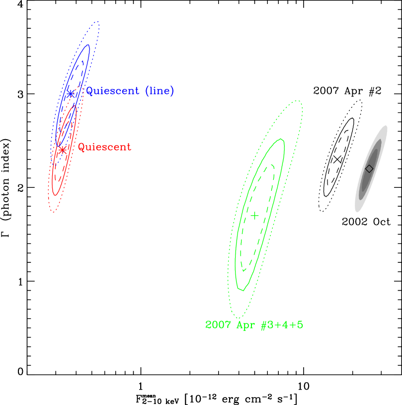
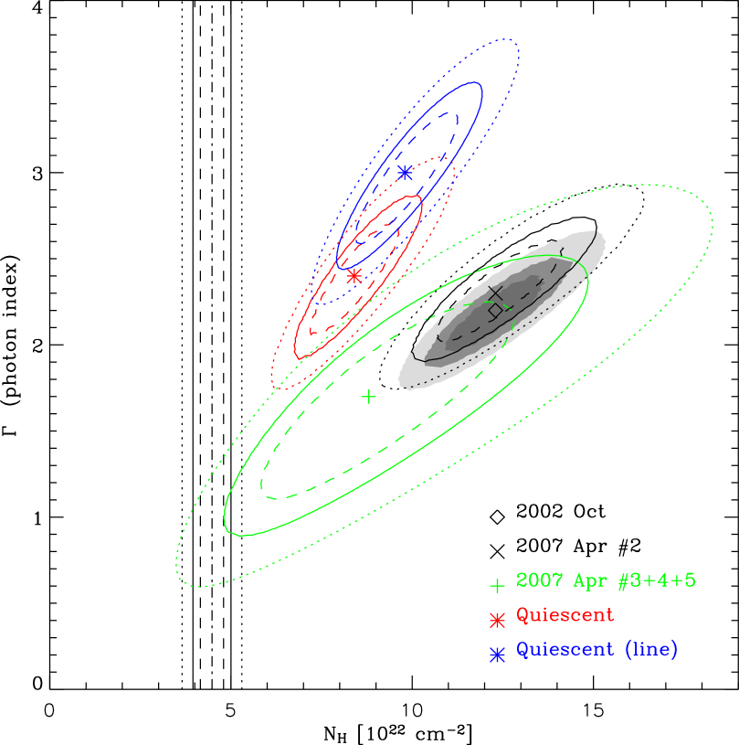
Figure 5: Confidence regions of the spectral parameters of the X-ray flares from Sgr A* for an absorbed power-law model taking into account the dust scattering. Left panel: photon index versus unabsorbed flux in the 2–10 keV energy range. The dashed, continuous, and dotted contour levels correspond to confidence levels for two interesting parameters of 68$\%$, 90$\%$, 99$\%$, respectively (i.e., to $\Delta C$ = 2.3, 4.61, 9.21, respectively). The confidence regions corresponding to the quiescent state of Sgr A* are inferred from the spectral analysis of four archived Chandra observations, using the same spectral models (red contour levels) or including a Gaussian emission line (blue contour levels). See text for details. Right panel: photon index versus column density. The dashed-dotted vertical line indicates the column density (4.5$\times 10^{22}$ cm^-2) derived from the $K$-band extinction value toward Sgr A* (2.8 mag with one-sigma uncertainty of 0.2 mag; Eisenhauer et al. 2005) using the extinction law of Rieke & Lebofsky (1985) and the empirical relation of Predehl & Schmitt (1995); the dashed, continuous, and dotted vertical lines correspond to 68$\%$, 90$\%$, 99$\%$ confidence levels, respectively.

4 Comparison of the spectral parameters of the X-ray flares observed up-to-now with XMM-Newton

Until now, the comparisons of X-ray flares from Sgr A* published in the literature have been based on spectral parameters obtained with different methods (e.g., different version of the SAS and CCF, different definition of flare time interval, scattering effect taken into account or not, etc). Here, we compare the spectral properties of the April 2007 flares (#2 and #3+#4+#5) with those of the rapid X-ray flares observed previously with XMM-Newton that we obtained using exactly the same method.

4.1 Reprocessing and spectral analysis of X-ray flares previously observed with XMM-Newton

We have reprocessed the observations of October 3, 2002 (orbit 516, ObsID: 0111350301; Porquet et al. 2003) and March 31, 2004 (orbit 789, ObsID: 0202670601; Bélanger et al. 2005) with the SAS version 7.1 and the latest CCF (see Appendix C). We did not reprocess the X-ray flare observed on September 4, 2001, because only a part of the beginning of the flare was observed (Goldwurm et al. 2003). We did not consider here the X-ray flare observed on August 31, 2004 (Bélanger et al. 2005) because it was contaminated by an X-ray transient in outburst, located at only 2.9″-South from Sgr A*, displaying dips/eclipses at this epoch (Muno et al. 2005; Porquet et al. 2005), which precludes the secure determination of the spectral parameters in this case.

The reprocessed light curves of the October 2002 and March 2004 flares are shown in the online Fig. 7. The time intervals of the flares have been defined using the same criteria used in $\S$3.1, and reported in the online Table 6. As done above, the 10^′′-radius extraction region has been optimized in each instrument by determining the position of Sgr A* during the time interval of the flare. The flare time interval found here for the October 2002 flare is very similar to the one used in Porquet et al. (2003). While, the flare time interval for the March 2004 found here using a time bin of 150 s is shorter ( 1200 s) than the time interval determined in Bélanger et al. (2005) using a much large time bin ($\sim$ 500 s), which contained a significant contribution of the non-flaring state.

We fitted the corresponding EPIC background-subtracted unbinned spectra with an absorbed power law model including dust scattering ($A_{\rm V}$=25 mag) and the $W$ statistic as for the flares $\#$2 and $\#$3+$\#$4+$\#$5 ($\S$3.2). In the October 2002 observation, the non-flaring period before the flare is too short ($\sim$10 ks) to allow a correct determination of the complex shape of the background spectrum of the non-flaring level, which is crucial when using $W$ statistic to fit the data. Therefore, we have used the longer observation of February 2002 (orbit 406, ObsID: 0111350101) where no Sgr A* flare were observed. Indeed, the non-flaring spectrum observed on February 2002 has the same shape and flux than the non-flaring spectrum observed on October 2002 before the flare, but it much more well constrained. We notice that using the $\chi^{2}$ statistic, using background spectra based either on the October 2002 observation or on the February 2002 observation, no impact on the parameter fits are found.

For the October 2002 flare the best fit parameters are reported in Table 3. The online Fig. 8 shows for illustration purpose the corresponding background-subtracted binned spectra and best-fit model for an absorbed power-law model using the $\chi^{2}$ statistic. As for the flare $\#2$, fits with the $\chi^{2}$ statistic give very similar parameter fits (see Table 5). Although, the central value of the photon index, $\Gamma$=2.2 ($\pm$0.3), is slightly lower than the value, $\Gamma$=2.5 ($\pm$0.3), previously reported by Porquet et al. (2003), both values are consistent when taking into account the error bars at the 90$\%$ confidence level. For this flare, both the position of Sgr A* during the flare and the flare time interval used in Porquet et al. (2003) were very similar to those used here, and then, are not responsible for the small difference in the central value of the photon index found here. Since the first analysis of the brightest flare by Porquet et al. (2003) with the SAS version 5.4, the cross-calibration between MOS and pn has been substantially improved (see e.g., http://xmm.vilspa.esa.es/docs/documents/CAL-TN-0018.psXMM-CAL-TN-0018). We checked that using the same extractions region, flare and background time intervals as used in Porquet et al. (2003) and the new calibration used in this work, we retrieved $\Gamma\sim$2.2.

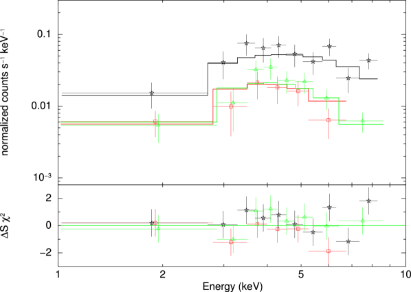
Figure 9: Same as Fig. 8 but for the flare observed on March 2004.

For the moderate flare observed on March 31, 2004, we found $N_{\rm H}$=4.5${}^{+3.4}_{-2.2}$$\times$10²² cm^-2 and $\Gamma$=0.8$\pm$0.6 (C/d.o.f.=1860/2998). Similar values are obtained with the $\chi^{2}$ statistic ($N_{\rm H}$=4.7${}^{+4.6}_{-3.0}$$\times$10²² cm^-2 and $\Gamma$=0.9${}^{+1.0}_{-0.9}$, $\chi^{2}$/d.o.f.=18.4/21; see Fig. 9). This central photon index value is smaller than the one reported by Bélanger et al. (2005) ($\Gamma$=1.5${}^{+0.5}_{-0.6}$ with the error bars calculated at the 68$\%$ confidence level), though compatible within the large error bars. The difference is mainly due to the method used here: a better determination of the flare time interval, which helps to decrease the contribution of the non-flaring level; a spectral fit done without binning the spectra when using the $W$ statistic, in order to not loose spectral information and then to not bias the parameter fit result; the dust scattering effect taken into account. A closer look to the fit of the March 2004 spectra show that when the instruments are fitted separately, very different central fit values are obtained (although compatible within the very large error bars). Moreover, the inferred column density value is lower than the one determined during the quiescent state (see below) and therefore appears unphysically low. When the column density is fixed to the value found for the brightest flares, the spectral index is 1.8$\pm$0.4 using the $W$ statistic (C/d.o.f=1872/2999) and 2.3$\pm$0.6 using the $\chi^{2}$ statistic ($\chi^{2}$/d.o.f.=24/22), which is consistent within the error bars with the spectral index value of the brightest flares. Therefore, we conclude that the spectral properties of this moderate flare are poorly constrained, and we will not considered it in our comparison of the flare properties.

4.2 Confidence regions of the spectral parameters

We show in the left and right panels of Fig. 5 the contour plot of the confidence regions of the photon index versus the unabsorbed flux and the column density, respectively, at the confidence levels of 68%, 90%, and 99% (corresponding to $\Delta C$=2.3, 4.61, and 9.21, respectively, for two interesting parameters). The fluxes of the flares span a large range, i.e., about a factor 5. The flare $\#$2 has a flux lower than the October 2002 flare at the 90% confidence level, but has similar best fit values of column density and spectral index. Due to a lower S/N, the physical parameters of the sum of the moderate flares (#3+#4+#5) are less constrained, but has column density and spectral index values compatible (within the error bars) with those of the bright flares.

The column density values during the flares are at least two times higher than the value expected from the 25 mag of (dust) visual extinction toward Sgr A*, i.e., 4.5$\times 10^{22}$ cm^-2. To know whether this excess of (gas) column density is related to the flare phenomena itself, we need to estimate the column density of the quiescent spectrum of Sgr A* with the same spectral model. However, the quiescent emission of Sgr A* can only be resolved with Chandra. The spectral properties of the quiescent emission of Sgr A* was reported by Baganoff et al. (2003), based on the first Chandra observations of the Galactic Center obtained in 1999 with a total effective exposure of about 41 ks. More Chandra observations of Sgr A* are now available in the archives. Starting from the level 2 of the archive event lists, we used CIAO 4.0 and CALDB 3.4.2 to produce Chandra X-ray light curves of Sgr A*. We selected four Chandra observations where Sgr A* displayed no flares. We extracted the corresponding quiescent spectra following the method of Baganoff et al. (2003); we refined the background 10$\arcsec$-radius extraction region by excluding the candidate pulsar wind nebula G359.95-0.04.

We have performed the simultaneous spectral analysis of these four quiescent spectra of Sgr A* obtained with Chandra. First, we fit the data with an absorbed power-law model using the $\chi^{2}$ statistic and a spectral binning of 10 counts per bin as done in Baganoff et al. (2003). When the dust scattering is not taken into account, we found $N_{\rm H}$=9.7${}^{+1.8}_{-1.5}\times$ 10²² cm^-2 and $\Gamma$=2.5${}^{+0.5}_{-0.4}$ ($\chi^{2}$/d.o.f.=143/130) and an unabsorbed 2–10 keV flux of 2.8${}^{+0.6}_{-0.4}\times$10^-13 erg cm^-2 s^-1. These values are similar to those reported by Baganoff et al. (2003) but are better constrained. An excess of emission is seen near 6.5 keV, therefore we add a Gaussian emission line and found $N_{\rm H}$=11.1${}^{+2.1}_{-1.9}\times$10²² cm^-2 and $\Gamma$=3.0${}^{+0.5}_{-0.6}$ and an unabsorbed 2–10 keV flux of 3.2${}^{+0.6}_{-0.7}\times$10^-13 erg cm^-2 s^-1, E_line=6.61${}^{+0.10}_{-0.10}$ keV, $\sigma_{\rm line}$=0.15${}^{+0.10}_{-0.12}$ keV, and $EW_{\rm line}$=1.1${}^{+0.4}_{-0.5}$ keV ($\chi^{2}$/d.o.f.=123/127). As found by Baganoff et al. (2003), we found a steeper power-law slope when an emission line is added to the fit. In this work, thanks to a much longer exposure time, we are able to constrain the line energy, which is consistent with a He-like iron line.

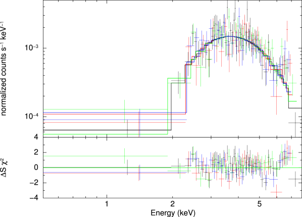
Figure 6: Chandra quiescent spectra of Sgr A*. Black, red, green, and blue data points correspond to ObsID 3665, 4683, 5950, and 5951, respectively. The lines show the best-fit model ($\chi^{2}$ statistic) using an absorbed power-law model taking into account the dust scattering. The fit residuals are shown in the bottom panel.

For illustration purpose, we show in Fig. 6 the background-subtracted binned Chandra spectra and the data/model fit residuals obtained for an absorbed power-law model taking into account the dust scattering effect with the $\chi{{}^{2}}$ statistic. To perform a homogeneous comparison with the spectral analysis of the XMM-Newton X-ray flares reported in this work, we then fit the unbinned Chandra quiescent spectra using the $W$ statistic and we took into account dust scattering effect. We found $N_{\rm H}$=8.4${}^{+1.4}_{-1.3}$$\times$ 10²² cm^-2, $\Gamma$=2.4${}^{+0.4}_{-0.4}$ ($C$/d.o.f.=1825/2457), corresponding to an unabsorbed 2–10 keV flux of 3.3${}^{+0.5}_{-0.4}\times$10^-13 erg cm^-2 s^-1 and a luminosity of 2.4${}^{+0.4}_{-0.3}\times$10³³ erg s^-1 (assuming d=8 kpc), similar to the value reported by Baganoff et al. (2003). The contour plots corresponding to this fit are reported on Fig. 5. If we add a Gaussian emission line we found $N_{\rm H}$=9.8${}^{+1.8}_{-1.5}\times$ 10²² cm^-2, $\Gamma$=3.0$\pm$0.5, E_line=6.67${}^{+0.05}_{-0.07}$ keV, $\sigma_{\rm line}\leq$0.19 keV, and $EW_{\rm line}$=0.9${}^{+0.4}_{-0.3}$ keV (C/d.o.f.=1781/2454). As shown in Fig. 5, the column density and power-law index values found for the quiescent state (Gaussian line added or not to the fit), are compatible, within the error bars calculated at 90% confidence level for two interesting parameters, with those found for the bright flares.

5 Summary and discussions

Here, we reported the data analysis of the XMM-Newton April 2007 campaign observation of Sgr A* (three observations with a total of exposure of $\sim$230 ks). We observed four X-ray flares occurring within only half a day on April 4: one bright flare ($\#2$, with a detection level of $\sim$21$\sigma$) followed by three moderate ones ($\#3$, $\#4$, and $\#5$, with a detection level of $\sim$6$\sigma$, $\sim$6$\sigma$, and $\sim$8$\sigma$, respectively). As well a weak flare ($\#1$, with a detection level of $\sim$3$\sigma$) was observed on April 2, 2007. The flare $\#2$ is the second brightest X-ray flare detected so far from Sgr A* and has a similar duration ($\sim$3 ks) to that of the October 2002 brightest flare (Porquet et al. 2003). Its light curve is almost symmetrical but without no significant short-time scale drop (i.e., about 50% of flux decrease) contrary to that reported for the October 2000 flare (Baganoff et al. 2001) and the October 2002 flare (Porquet et al. 2003). However, for the flare $\#$2 we cannot rule out a moderate drop in the X-ray light curve. A similar group of three moderate flares were already observed with XMM-Newton on 2004 March 31 (Bélanger et al. 2005), but no such preceding bright flare was observed.

This is the first time that a such level of X-ray flaring activity from Sgr A*, both in amplitude and frequency, is reported. Observations such as those reported in this paper can eventually constrain flare models in Sgr A*, perhaps even ruling some out. For example, the quick succession of several events separated by only a few hours, might argue against a disruption mechanism that relies on the temporary storage of mass and energy, if all the corresponding accretion energy is released during the flare. The accretion rate $\dot{M}$ in this system (some estimates place it as low as $10^{16}-10^{17}$ g s^-1; see Melia 2007) might not produce a transient accumulation of mass $\Delta M$ between flares of sufficient magnitude for $\eta GM\Delta M/3R_{S}$ to provide the observed outburst power. In this expression, $R_{S}$ is the Schwarzschild radius, and $\eta$ is the (poorly known) radiative efficiency in Sgr A*, believed to be at most a few percent. If instead the flares are due to a magneto-rotational instability, then the energy liberated during the flare must also be accumulated over the short inter-burst period. The low $\dot{M}$, from which the energy is derived, might argue against this type of mechanism as well.

On the other hand, if the flare arises from the infall of a clump of gas (e.g., Liu et al. 2006; Tagger & Melia 2006) then there would be less restriction on how often these could come in. Genzel et al. (2003) have shown that the total energy release $\geq$ 10^39.5 erg during a flare requires a gas accreted mass of a few times 10¹⁹ g (assuming a radiation efficiency of $\sim$10$\%$), i.e. comparable to that of a comet or a small asteroid. Recently, Cadež et al. (2006) have argued that the flares could be produced by tidal captures and disruptions of such small bodies. The comet/asteroid/planetesimal idea for depositing the additional mass and energy to initiate a flare is attractive. The distance from Sgr A* at which such a small body would get tidally disrupted is the Roche radius, which is for a rigid body:

$$\frac{R_{\cal R}}{R_{\rm S}}=13.2\times\left(\frac{M_{\rm BH}}{4\times 10^{6}M_{\odot}}\right)^{-2/3}\times\left(\frac{\rho_{p}}{{\rm 1\,g\,cm^{-3}}}\right)^{-1/3}\,,$$

where $M_{\rm BH}$ is the black hole mass and $\rho_{p}$ is the density of the rigid body. Thus, for a black-hole mass of $4\times 10^{6}\;M_{\odot}$ and a density of 1 g cm^-3, this corresponds to $13.2\,R_{\rm S}$, in good agreement with the size of the region where the flares are thought to occur. The flaring rates would then depend on processes occurring much farther out, so the fact that so many flares are seen so close together on some days, and much less frequently at other times, would simply be due to stochastic events. However, it would still be difficult to distinguish between a compact emission region and emission within a jet (see, e.g., Markoff et al. 2001), since these disruption events could still end up producing an ejection of plasma associated with the flare itself.

Four of the five X-ray flares observed during this campaign have a simultaneous NIR flare counterpart: flares $\#1$, $\#4$, and $\#5$ were observed with HST/NICMOS (Yusef-Zadeh et al. 2008, in prep.); and flare $\#2$ was observed with VLT/NACO (Dodds-Eden et al. 2008, in prep.). The flare $\#3$ has not been covered by a simultaneous NIR observation. This strengthens the relationship observed up to now between X-ray and NIR flares when there is a simultaneous X-ray/NIR observation coverage: all X-ray flares have an NIR flare counterpart, while all NIR flares are not each time associated with an X-ray flare counterpart (e.g., Eckart et al. 2004, 2006; Yusef-Zadeh et al. 2006; Hornstein et al. 2007; Marrone et al. 2008).

We have made the first detailed comparison of X-ray flare properties observed with XMM-Newton (this April 2007 campaign and previous observations) based on a fully self-consistent analysis approach, namely we use the same SAS version with the latest calibration, the same definition of the flare interval (preventing from significant contribution of the non-flaring level), an optimized extraction region for each instrument, and we took into account the dust scattering effect. We found that the physical parameters of the flare $\#2$, $N_{\rm H}$=12.3${}^{+2.1}_{-1.8}$$\times$ 10²² cm^-2 and $\Gamma$=2.3$\pm$0.3, are well constrained and are very similar to that of the October 2002 (brightest) flare, $N_{\rm H}$=12.3${}^{+1.6}_{-1.5}$$\times$10²² cm^-2 and $\Gamma$=2.2$\pm$0.3. The spectral parameter fit values of the sum of the three moderate flares following the bright flare observed on April 4, 2007, $N_{\rm H}$=8.8${}^{+4.1}_{-3.2}$$\times$ 10²² cm^-2 and $\Gamma$=1.7${}^{+0.7}_{-0.6}$, while lower, are compatible within the error bars with those of the bright flares. The column density found during the bright flares is at least two times higher than the value expected from the (dust) visual extinction toward Sgr A* ($A_{\rm V}\sim 25$ mag; Eisenhauer et al. 2005), i.e., 4.5$\times 10^{22}$ cm^-2. However, our fitting of the Sgr A* quiescent spectra obtained using four Chandra observations for a total observation time of $\sim$ 230 ks, taking into account the dust scattering, shows that a column density excess is already present during the non-flaring phase. One possible explanation, as already pinpoint by Maeda et al. (2002), is that such column density excess in the line-of-sight of Sgr A* could be due to the warm (dust free) gas associated with the ionized gas halo, Sgr A West extended, suggested by the turnover absorption observed at 90 cm, embedded the Sgr A complex (e.g., Pedlar et al. 1989; Anantharamaiah et al. 1999; Yusef-Zadeh et al. 2000). Anantharamaiah et al. (1999) inferred that this ionized halo has a dimension of about 4$\arcmin$ ($\sim$9pc) and an electron density of about 100–1000 cm^-3. For a column excess of about 2.9$\times$10²² cm^-2 as found for the Sgr A* quiescent state, this would correspond to a consistent electron density of about 1300 cm^-3. However, in case the genuine continuum shape is curved compared to a power law and bremsstrahlung models, as for example a black body like shape, no significant column excess would be required.

On the basis of our current analysis we conclude that the dichotomy of the spectral index between moderate and bright flares (i.e., a correlation between photon index and flux) suggested by Bélanger et al. (2005) is not confirmed. However, to test this more thoroughly we need further observations so as to extend the sampling of the flaring activity seen from Sgr A* (and in particular those instances where good signal to noise can be achieved through the co-adding of weak to moderate flaring events).

In conclusion, this study establishes that the two brightest X-ray flares observed so far from Sgr A* exhibited similar (well constrained) soft spectra. Therefore, any model proposed to explain the flaring behavior of Sgr A* must take into account this observational X-ray spectral property.

Appendix A Absolute astrometry of the bright X-ray flare

To obtain an absolute astrometry of the bright X-ray flare, we registered the positions of the soft X-ray sources in the third observations on the Hipparcos celestial coordinate system using the X-ray counterparts of the Tycho-2 catalog’s sources (Høg et al. 2000). We matched the positions of the pn sources detected in the 0.5–1.5 keV energy band obtained with the SAS task edetect_chain with the positions of Tycho-2 catalog’s sources for the epoch of our observation. We found 4 X-ray counterparts of Tycho-2 sources using a cross-correlation radius of $5\arcsec$. The X-ray counterpart of Tyc 6840 020 1, lying on a pn CCD gap, is not considered in the following. The offsets between pn and Tycho-2 positions of these three reference sources shows a systematic translation. The weighted mean offset is $-0\aas@@fstack{\prime\prime}7$ and $0\aas@@fstack{\prime\prime}6$ in right ascension and declination, respectively. Therefore, we correct the X-ray position by subtracting this weighted mean offset. The residual RMS scatter in the corrected X-ray positions of the reference sources, $0\aas@@fstack{\prime\prime}9$, gives the astrometric uncertainty of the registration. This value is combined with the positional error of the PSF fitting to derived the final positional uncertainty. We list in Table 4 the corrected X-ray positions of the Tycho-2 reference stars, the final positional uncertainties, and the distance to the Tycho-2 optical positions. The absolute position of the X-ray bright flare is $\alpha_{\rm J2000}=17^{\rm h}45^{\rm m}40.0^{\rm s}$, $\delta_{\rm J2000}=-29^{\circ}00^{\prime}28.6^{\arcsec}$ with a one-sigma positional uncertainty of $1\aas@@fstack{\prime\prime}0$.

Table 4: X-ray counterparts of Tycho-2 reference stars.

Name	J2000 coordinates(a)	Err.(b)	Name	Dist.
XMMU J1745	$17^{\rm h}45^{\rm m}$	$\arcsec$	Tyc 6840	$\arcsec$
25.7-285627	$25.7^{\rm s}$ $-28^{\circ}56^{\prime}27.8^{\arcsec}$	1.3	666 1	0.9
43.8-291317	$43.8^{\rm s}$ $-29^{\circ}13^{\prime}17.7^{\arcsec}$	1.7	334 1	0.9
43.9-290456	$43.9^{\rm s}$ $-29^{\circ}04^{\prime}56.5^{\arcsec}$	1.1	590 1	0.2

• Absolute position corrected from systematic translation.
  

• Final positional uncertainty obtained by combining the positional error of the PSF fitting with the astrometric uncertainty of the registration on Tycho-2 sources.
  

Appendix B $\chi{{}^{2}}$ statistic versus $W$ statistic

The flare spectra are rebinned from 1 keV using grppha to have at least 25 counts per spectral bin. We ignore data above 10 keV, as for the fits with the W statistic (see $\S$3.2). XSPEC (version 12.4.0; Arnaud 1996) was used to fit the background-subtracted spectrum. For the October 2002, as for the $W$ statistic spectral fit, we used as background the longer February 2002 observation (orbit 406, ObsID: 0111350101) where no Sgr A* flare were observed. If the non-flaring spectrum observed on October 2002 before the flare is used as background, very similar parameter fits are obtained. The errors and upper limits quoted correspond to 90$\%$ confidence level for one interesting parameter. The parameter fits (see Table 5) are similar to that found using the $W$ statistic for bright flares. For lower S/N flares the central values are different but consistent within the error bars with that the values found using $W$ statistic. The error bars are generally larger using the $\chi{{}^{2}}$ statistic.

Table 5: Best fit parameters (using $\chi^{2}$ statistic) of the EPIC flare spectra for absorbed pegged power-law (pow), bremsstrahlung (brems), and black-body (bb) models, taking into account dust scattering (assuming A_v=25 mag). The errors are given at the 90% confidence level.

Flare	Model	$N_{\rm H}^{\rm\,(a)}$	$\Gamma$/kT(b)	$F^{\rm mean(c)}_{2-10\,{\rm keV}}$	$\chi^{2}$/d.o.f.	$\cal{Q}^{\rm(d)}$
April 4, 2007
$\#2$	pow	12.8${}^{+2.5}_{-2.1}$	2.3${}^{+0.4}_{-0.4}$	15.7${}^{+3.6}_{-2.4}$	70.2/75	63.6$\%$
	brems	11.3${}^{+1.9}_{-1.6}$	6.8${}^{+3.7}_{-1.9}$	13.4${}^{+5.2}_{-3.1}$	69.8/75	64.9$\%$
	bb	7.3${}^{+1.6}_{-1.3}$	1.5${}^{+0.1}_{-0.1}$	9.5${}^{+0.8}_{-0.7}$	71.5/75	59.2$\%$
$\#3$+$\#4$+$\#5$(e)	pow	6.3${}^{+4.6}_{-2.8}$	1.2${}^{+0.7}_{-0.6}$	4.1${}^{+1.3}_{-0.7}$	29.9/32	57.3$\%$
	brems	6.4${}^{+2.3}_{-1.6}$	$\geq$ 11	4.1${}^{+6.6}_{-1.4}$	29.9/32	57.4$\%$
	bb	2.9${}^{+2.6}_{-1.7}$	2.1${}^{+0.6}_{-0.4}$	3.3${}^{+1.2}_{-0.7}$	29.7/32	58.2$\%$
October 3, 2002
	pow	12.1${}^{+1.7}_{-1.5}$	2.2${}^{+0.3}_{-0.3}$	24.1${}^{+3.6}_{-2.7}$	90.4/102	78.8$\%$
	brems	10.6${}^{+1.3}_{-1.1}$	7.9${}^{+3.4}_{-1.9}$	20.9${}^{+5.2}_{-3.6}$	90.9/102	77.6$\%$
	bb	6.5${}^{+1.1}_{-1.0}$	1.6${}^{+0.1}_{-0.1}$	14.9${}^{+0.8}_{-0.8}$	98.1/102	59.0$\%$

• $N_{\rm H}$ is units of 10²² cm^-2.

• The black-body temperature is given in keV.

• Mean unabsorbed fluxes for the flare period in the 2–10 keV energy range in units of 10^-12 erg cm^-2 s^-1.

• $\cal{Q}$ is the null hypothesis probability, i.e., the probability of getting a value of $\chi^{2}$ as large or larger than observed if the model is correct.

• These parameter fits for flare $\#3$+$\#4$+$\#5$ are only given to illustrate the impact on both the central parameter fit values and the constraints on error bars, when using $\chi^{2}$ statistics in case of low statistics, instead of $W$ statistics (see Table 3 for comparison).

Appendix C Reprocessed light curves and spectra of the X-ray flares previously observed with XMM-Newton

We report the reprocessed light curves (Fig. 7) and spectra (Fig. 8 and 9) of the X-ray flares observed on October 2002 and March 2004 that were reported previously by Porquet et al. (2003) and Bélanger et al. (2005), respectively. Table 6 gives for each flare: the start and end times, the duration, the total EPIC quiescent-subtracted counts, and EPIC quiescent-subtracted count rate at the peak flare.

The X-ray flare observed on March 2004 was contaminated by a high level of background proton flares which lead for pn to numerous switches between science and counting mode, and therefore to a significant loss of exposure time. Consequently, a bin time interval of 100 s contains less than 50% of (scientific mode) exposure, which is not enough to obtain a good estimate of the count rate. We used a bin time interval of 150 s, which is sufficient to obtain a good estimate of the count rate, when comparing with the MOS light curves. Obviously, this loss of exposure on this moderate flare affected the quality of its pn spectrum, and the resulting constraints derived on its physical parameters.

Figure 7: Light curves of reprocessed X-ray anterior flares observed with XMM-Newton. Left: October 2002 flare. Right: March 2004 flare.

Table 6: Characteristics of the X-ray flares observed in October 2002 and March 2004 (see Fig.  7).

Flare	Start time(a)		End time(a)		Duration	Total(b)	Peak(c)	Det.(d)	$L_{\rm 2-10\leavevmode\nobreak\ keV}^{\rm peak\leavevmode\nobreak\ (e)}$	Ampl.(f)
	hh:mm:ss	s	hh:mm:ss	s	s	cts	cts s-1	$\sigma$	1034 erg s-1
03/10/2002	10:07:40	150026860	10:54:20	150029660	2800	2158	1.510	29.6	35.9${}^{+7.1}_{-5.2}$	(g)149${}^{+21}_{-16}$
31/03/2004	22:52:24	197160744	23:12:24	197161944	1200	447	0.653	12.8	11.0${}^{+0.2}_{-0.2}$	46${}^{+9}_{-15}$

• Start and end times of the flare time interval defined as the period where the EPIC light curve deviates from the non-flaring level at a confidence of 95%. See $\S$3.1 for details.

• Total EPIC counts in the 2–10 keV energy band obtained during the flare interval after subtraction of the non-flaring level.

• EPIC count rate in the 2–10 keV energy band at the flare peak after subtraction of the non-flaring level.

• Detection level at the flare peak in $\sigma$.

• 2–10 keV luminosity at the flare peak, assuming an absorbed power law model (taking account dust scatter effect), see parameter fits in Table 3.

• Amplitude of the flare defined as the ratio of the 2–10 keV flare luminosity at the peak and the 2–10 keV quiescent luminosity of Sgr A* observed with Chandra (i.e., 2.4 $\times$ 10³³ erg s^-1, Baganoff et al. 2003, and this work, see $\S$4).

• In Porquet et al. (2003), the amplitude was calculated using the 2–10 keV quiescent luminosity of Sgr A* reported in Baganoff et al. (2001), i.e. 2.2 $\times$ 10³³ erg s^-1. Using this latter quiescent luminosity value, we would find for October 2002, an amplitude of 163${}^{+23}_{-17}$.

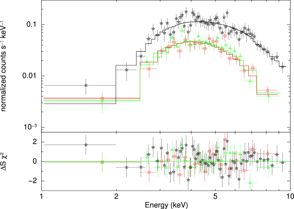
Figure 8: XMM-Newton EPIC spectra of the flare observed on October 2002. The spectrum for the non-flaring period with the same extraction region is used as background. Squares, triangles and stars indicate MOS1 (red), MOS2 (green), and pn (black) data, respectively. The lines show the best-fit model using an absorbed power-law model taking into account dust scattering (see Table 5 for best fit parameter values; pow model). The fit residuals are shown in the bottom panels.