On the product of two gamma variates with argument 2: Application to the luminosity function for galaxies.

Abstract

A new luminosity function for galaxies can be built starting from the product of two random variables X and Y represented by a gamma variate with argument 2 . The mean , the standard deviation and the distribution function of this new distribution are computed. This new probability density function is assumed to describe the mass distribution of galaxies. Through a non linear rule of conversion from mass to luminosity a second new luminosity function for galaxies is derived. The test of reliability of these two luminosity functions was made on the Sloan Digital Sky Survey (SDSS) in five different bands. The Schechter function gives a better fit with respect to the two new luminosity functions for galaxies here derived.

02.50.Cw Probability theory; 98.62.Ve Statistical and correlative studies of properties (luminosity and mass functions; mass-to-light ratio; Tully-Fisher relation, etc.)

1 Introduction

Given two independent non-negative random variables X and Y, their product XY represents an active field of research. When X and Y are Student’s $t$ random variables the product XY is applied in the field of finance [1] . When X and Y are n-Rayleigh distribution , the application can be the wireless propagation research [2] . In Section 2 this paper explores the product XY when X and Y are gamma variate with argument 2. Section 3 explores the connection between the Voronoi Diagrams and galaxies. Section 4 reports two new luminosity functions for galaxies as deduced from the product XY.

2 The new distribution of probability

The starting point is the probability density function ( in the following PDF) in length , $s$ , of a segment in a random fragmentation

$$p(s)=\lambda\exp{(-\lambda s)}ds\quad,$$ (1)

where $\lambda$ is the hazard rate of the exponential distribution. Given the fact that the sum , $u$ , of two exponential distributions has PDF

$$p(u)=\lambda^{2}u\exp{(-\lambda u)}du\quad.$$ (2)

The PDF of the $1D$ Voronoi segments , $l$, ( the midpoint of the sum of two segments) can be found from the previous formula inserting $u=2l$

$$p(l)=2\lambda l\exp{(-2\lambda l)}d(2\lambda l)\quad.$$ (3)

On transforming in normalized units $x=\frac{l}{\lambda}$ we obtain the following PDF

$$p(x)=2x\exp{(-2x)}d(2x)\quad.$$ (4)

When this result is expressed as a gamma variate we obtain the PDF (formula (5) of [3])

$$H(x;c)=\frac{c}{\Gamma(c)}(cx)^{c-1}\exp(-cx)\quad,$$ (5)

where $0\leq x<\infty$ , $c~{}>0$ and $\Gamma(c)$ is the gamma function with argument c; in the case of $1D$ Voronoi Diagrams $c=2$. It was conjectured that the area in $2D$ and the volumes in $3D$ of the Voronoi Diagrams may be approximated as the sum of two and three gamma variate with argument 2. Due to the fact that the sum of n independent gamma variates with shape parameter $c_{i}$ is a gamma variate with shape parameter $c=\sum_{i}^{n}c_{i}$ the area and the volumes are supposed to follow a gamma variate with argument 4 and 6  [4, 5]. This hypothesis was later named ”Kiang’s conjecture”, and equation (5) was used as a fitting function , see [6, 7], or as an hypothesis to accept or to reject using the standard procedures of the data analysis, see [8, 9]. PDF (5) can be generalized by introducing the dimension of the considered space, $d(d=1,2,3)$,

$$H(x;d)=\frac{2d}{\Gamma(2d)}(2dx)^{2d-1}\exp(-2dx)\quad.$$ (6)

Two other PDF are suggested for the Voronoi Diagrams:

• The generalized gamma function with three parameters $(a,b,c)$

  $$f(x;b,c,d)=c\frac{b^{a/c}}{\Gamma(a/c)}x^{a-1}\exp{(-bx^{c})}\quad,$$ (7)

  see [9], [10].

• A new analytical PDF of the type

  $$FN(x;d)=Const\times x^{\frac{3d-1}{2}}\exp{(-(3d+1)x/2)}\quad,$$ (8)

  where

  $$Const=\frac{\sqrt{2}\sqrt{3\,d+1}}{2\,{2}^{3/2\,d}\left(3\,d+1\right)^{-3/2\,d}\Gamma\left(3/2\,d+1/2\right)}\quad,$$ (9)

  and $d(d=1,2,3)$ represents the dimension of the considered space , see [11].

Experimentally determined physical quantities are usually derived from combinations of measurements, each of which may be considered a random variable subject to a known distribution law. The distribution law of the sought-for physical quantity, however, is generally not known or determinable analytically, except for a linear superposition of random variables , i.e. the sum of n independent gamma variates, [12]. Physical quantities represented as products of random variables are of especial interest. Computer simulations of products of normally distributed random variables , as an example , lead to distributions that are not normal, in some cases markedly so with pronounced skewness, depending upon the parameters of the component distributions, [12]. Consider , for example, the product of two random variables $X\approx N(0,1)$ and the random variable $Y\approx N(0,1)$, the PDF of $V=XY$ is , see [13] ,

$$h(v)=\left\{\begin{array}[]{ll}K_{0}(v*signum(v))/\pi&-\infty<v<0\\ K_{0}(v*signum(v))/\pi&0<v<\infty~{}.\end{array}\right.$$ (10)

This PDF has a pole at $v=0$ .

We now explore the product of two gamma variate with argument 2. We recall that if $X$ is a random variable of the continuous type with PDF , $f(x)$, which is defined and positive on the interval $0\leq x<\infty$ and similarly if $Y$ is a random variable of the continuous type with PDF $g(y)$ which is defined and positive $0\leq y<\infty$ , the PDF of $V=XY$ is

$$h(v)=\int_{0}^{\infty}g(\frac{v}{x})f(x)\frac{1}{x}dx\quad.$$ (11)

Here the case of equal limits of integration will be explored , when this is not true difficulties arise [14, 13] . When $f(x)$ and $g(y)$ are gamma variates with argument 2 the PDF is

$$h(v)=\int_{0}^{\infty}\frac{16\,{e^{-2\,x}}v{e^{-2\,{\frac{v}{x}}}}}{x}dx=32\,v{\it K_{0}}\left(4\,\sqrt{v}\right)\quad,$$ (12)

where $K_{\nu}(z)$ is the modified Bessel function of the second kind [15, 16] with $\nu$ representing the order, in our case 0. The distribution function ( in the following DF) is

$$16\,{v}^{2}{\it K_{0}}\left(4\,\sqrt{v}\right){\it~{}_{2}F_{1}}\left(1,2;3;4\,v\right)+16\,{v}^{5/2}{\it K_{1}}\left(4\,\sqrt{v}\right){\it~{}_{2}F_{1}}\left(1,3;3;4\,v\right)\quad,$$ (13)

where ${~{}_{2}F_{1}(a,b;\,c;\,v)}$ is a regularized hypergeometric function, see [15, 17, 18].

The mean of the new PDF, $h(v)$, as represented by formula (12) is

$$<v>=\int_{0}^{\infty}v\times 32\,v{\it K_{0}}\left(4\,\sqrt{v}\right)dv=1\quad,$$ (14)

and the variance

$$\sigma^{2}=\int_{0}^{\infty}(v-1)^{2}\times 32\,v{\it K_{0}}\left(4\,\sqrt{v}\right)dv=\frac{5}{4}\quad.$$ (15)

The mode , $m$ , is at v =0.15067 . Figure 1 reports our function $h(x)$ as well the Kiang function $H(x;c)$ for three values of $c$.

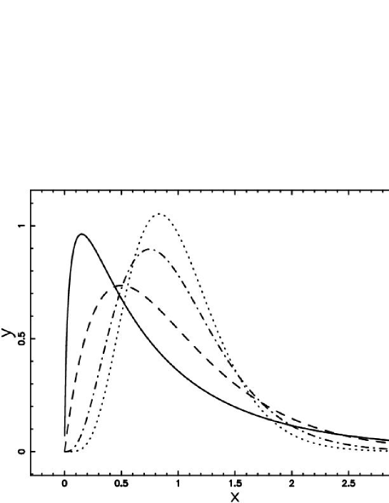
Figure 1: Plot of $h(x)$ as function of $x$ (full line) , H (x ;c ) when $c=2$ (dashed), H (x ;c ) when $c=4$ (dot-dash-dot-dash) and H (x ;c ) when $c=6$ (dotted).

Asymptotic series are

$$h(v)\sim-16\,\left(2\,\ln\left(2\right)+\ln\left(v\right)+2\,\gamma\right)v\quad v\ll 1\quad,$$ (16)

$$h(v)\sim-\frac{\sqrt{2}\sqrt{\pi}{e^{-{\frac{4}{\sqrt{\frac{1}{v}}}}}}\left(-32+\sqrt{\frac{1}{v}}\right)}{4\,\left(\frac{1}{v}\right)^{3/4}}\quad v\gg 1\quad,$$ (17)

where $\gamma$ is the Euler-Mascheroni constant.

3 Voronoi Diagrams and galaxies

The applications of the Voronoi Diagrams, see [19] and [20], in astrophysics started with  [3] where through a Monte Carlo experiment, the area distribution in 2D and volume distribution in 3D were deduced. The application of the Voronoi Diagrams to the distribution of galaxies started with [21], where a sequential clustering process was adopted in order to insert the initial seeds. Later a general algorithm for simulating one-dimensional lines of sight through a cellular universe was introduced [22]. The large microwave background temperature anisotropies over angular scales up to one degree were calculated using a Voronoi model for large-scale structure formation in [23] and [24]. The intersections between lines that represent the ’pencil beam’ surveys and the faces of a three-dimensional Voronoi tessellation has been investigated by [25] where an exact expression is derived for the distribution of spacings of these intersections. Two algorithms (among others) that allow to detect structures from galaxy positions and magnitudes are briefly reviewed :

• A Voronoi Galaxy Cluster Finder (VGCF) that uses galaxy positions and magnitudes to find clusters and determine their main features: size, richness and contrast above the background , see [26, 27].

• An automated procedure for structure finding, involving the Voronoi tessellation allows to build a catalogue (called PF) of galaxy structures (groups and clusters) in an area of 5,000 square degrees in the southern hemisphere, see [28, 29].

This section first explores how the fragmentation of a 2D layer as due to the 2D Voronoi Diagrams can be useful or not in describing the mass distribution of galaxies. The large scale structures of our universe are then explained by the 3D Voronoi Diagrams in the second section.

3.1 Mass distribution

Here we Analise the fragmentation of a 2D layer of thickness which is negligible with respect to the main dimension. A typical dimension of the layer can be found as follows. The averaged observed diameter of the galaxies is

$$\overline{D^{obs}}\approx 0.6{D_{max}^{obs}}=2700\frac{Km}{sec}=27~{}Mpc\quad,$$ (18)

where $D_{max}^{obs}=4500~{}\frac{Km}{sec}$ corresponds to the extension of the maximum void visible on the CFA2 slices. In the framework of the theory of the primordial explosions ,see [30] and [31], this means that the mean observed area of a bubble ,$\overline{A^{obs}}$, is

$$\overline{A^{obs}}\approx 4\pi(\frac{D_{max}^{obs}}{2})^{2}=2290Mpc^{2}\quad.$$ (19)

The averaged area of a face of a Voronoi polyhedron , $\overline{A_{V}}$, is

$$\overline{A_{V}}=\frac{\overline{A^{obs}}}{\overline{N_{F}}}\quad,$$ (20)

where ${\overline{N_{F}}}$ is the averaged number of irregular faces of the Voronoi polyhedron, i.e. ${\overline{N_{F}}}$=16 , see [32, 7]. The averaged side of a face of a irregular polyhedron , $L_{V}$ , is

$$\overline{L_{V}}\approx\sqrt{\overline{A^{obs}}}\approx 12~{}Mpc\quad.$$ (21)

The thickness of the layer , $\delta$ , can be derived from the shock theory , see [33], and is 1/12 of the radius of the advancing shock ,

$$\delta=\frac{{D_{max}^{obs}}}{2\times 12}\approx 1.12Mpc\quad.$$ (22)

The number of galaxies in this typical layer , $N_{G}$, can be found by multiplying $n_{*}\approx 0.1$ , the density of galaxies , by the volume of the cube of side 12 $Mpc$ : i.e. $N_{G}\approx 172$.

A first application of the new PDF, $h(v)$, as represented by formula (12) , can be a test on the area distribution of the Voronoi polygons , see Figure 2. Does the area distribution of the irregular polygons follow the sum or the product of two gamma variates with argument 2 ?. In order to answer this question we fitted the sample of the area with $h(v)$ , the new PDF , with a gamma variate with argument 4 and with a gamma variate with the argument as deduced from the sample. The results are reported in Table 1.

Table 1: The $\chi^{2}$ of data fit when the number of classes is 10 for three PDF

$$\begin{array}[]{lc}\hline\cr PDF&\chi^{2}\\ \vskip 3.0pt plus 1.0pt minus 1.0pt\cr\hline\cr\vskip 3.0pt plus 1.0pt minus 1.0pt\cr h(x)&62.8\\ \vskip 3.0pt plus 1.0pt minus 1.0pt\cr H(x;c)~{}when~{}c=4&28.3\\ \vskip 3.0pt plus 1.0pt minus 1.0pt\cr H(x;c)~{}when~{}c=3.7&23.55\\ \vskip 3.0pt plus 1.0pt minus 1.0pt\cr FN(x;d)~{}Ferenc~{}\&~{}Neda~{}formula~{}(\ref{rumeni})~{}when~{}d=2&20.2\\ \vskip 3.0pt plus 1.0pt minus 1.0pt\cr\hline\cr\hline\cr\end{array}$$

From a careful inspection of Table 1 it is possible to conclude that the area distribution of the irregular Voronoi polygons is better described by the sum of two gamma variates with argument 2 rather than by the product.

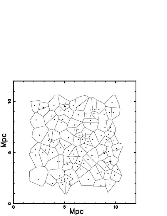
Figure 2: The Voronoi–Diagram in 2D when random seeds are used. The selected region comprises 102 seeds.

3.2 Spatial dependence

Our method considers a 3D lattice made of ${\it pixels}^{3}$ points : present in this lattice are $N_{s}$ seeds generated according to a random process. All the computations are usually performed on this mathematical lattice; the conversion to the physical lattice is obtained by multiplying the unit by $\delta=\frac{side}{pixels-1}$ , where side is the length of the square/cube expressed in the physical unit adopted. The tessellation in $\Re^{3}$ is firstly analyzed through a planar section . Given a section of the cube (characterized , for example, by $k=\frac{pixel}{2}$) the various $V_{i}$ (the volume belonging to the seed $i$) may or may not cross the little cubes belonging to the two dimensional lattice . Following the nomenclature introduced by [32] we call the intersection between a plane and the cube previously described as $V_{p}(2,3)$; a typical example is shown in Figure 3.

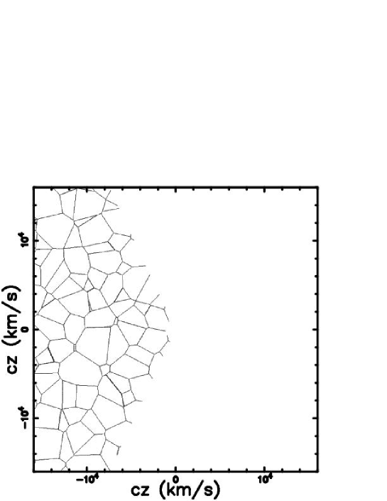
Figure 3: Portion of the Voronoi–Diagram $V_{p}(2,3)$ when random seeds are used; cut on the x–y plane  . For astronomical purposes we only report a slice $130^{\circ}$ long. The parameters are pixels = 800 , N = 1900 and side = 2 $\times$ 16000 Km/sec

For astronomical purposes is also interesting to plot the little cubes belonging to a slice of $6^{\circ}$ wide and about $130^{\circ}$ long, see Figure 4.

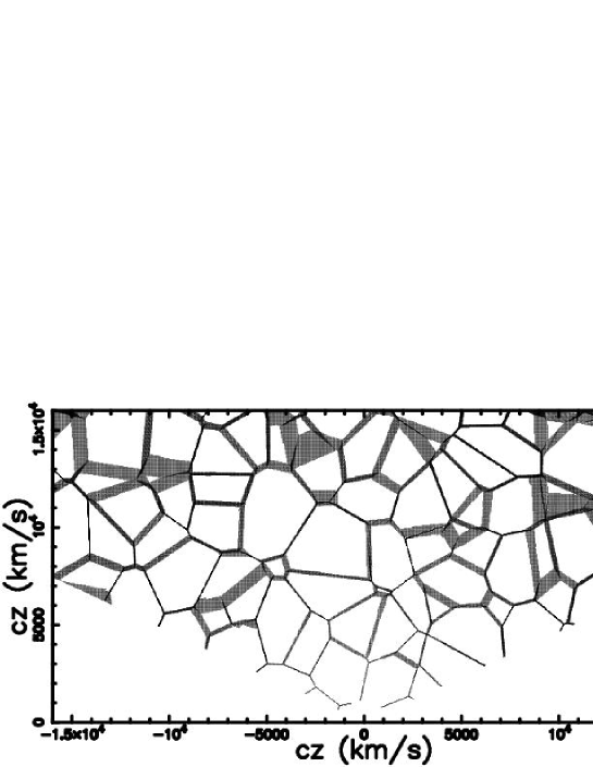
Figure 4: Polar plot of the little cubes belonging to a slice $130^{\circ}$ long and $6^{\circ}$ wide. Parameters as in Figure 3.

4 A new luminosity function for galaxies

The new PDF as given by formula (12) can represent a PDF in mass for the galaxies. The luminosity function , in the following LF, for galaxies is then deduced by introducing a linear and a non linear relationship between mass and luminosity. A special section is devoted to the parameters determination of the two new LF for galaxies. The dependence of the number of galaxies with the redshift is then analyzed by adopting the first new LF.

4.1 Schechter luminosity function

A model for the LF of galaxies is the Schechter function

$$\Phi(L)dL=(\frac{\Phi^{*}}{L^{*}})(\frac{L}{L^{*}})^{\alpha}\exp\bigl{(}{-\frac{L}{L^{*}}}\bigr{)}dL\quad,$$ (23)

where $\alpha$ sets the slope for low values of $L$ , $L^{*}$ is the characteristic luminosity and $\Phi^{*}$ is the normalization. This function was suggested by [34] in order to substitute other analytical expressions, see for example, formula (3) in [35]. Other interesting quantities are the mean luminosity per unit volume, $j$ ,

$$j=\int^{\infty}_{0}L\Phi(L)dl={\it L^{*}}\,{\it\Phi^{*}}\,\Gamma\left(\alpha+2\right)\quad,$$ (24)

and the averaged luminosity ,${\langle L\rangle}$ ,

$$\langle L\rangle=\frac{j}{\Phi^{*}}={\it L^{*}}\,\Gamma\left(\alpha+2\right)\quad,$$ (25)

where $\Gamma$ is the gamma function and its appearance is explained in [36]. An astronomical form of equation (23) can be deduced by introducing the distribution in absolute magnitude

$$\Phi(M)dM= (0.4ln10)\Phi^{*}10^{0.4(\alpha+1)(M^{*}-M)}$$ (26)

$$\times\exp\bigl{(}{-10^{0.4(M^{*}-M)}}\bigr{)}dM\quad,$$

where $M^{*}$ is the characteristic magnitude as derived from the data. At present this function is widely used and Table 2 reports the parameters from the following catalogs

• The 2dF Galaxy Redshift Survey (2dFGRS) based on a preliminary subsample of 45000 galaxies, see [37].

• The $r^{\ast}$-band LF for a sample of 11,275 galaxies from the Sloan Digital Sky Survey (SDSS) , see [38].

• The galaxy LF for a sample of 10095 galaxies from the Millennium Galaxy Catalogue (MGC) , see [39].

• The CFA Redshift Survey [40] that covered 9063 galaxies with Zwicky $m$ magnitude $<$ 15.5 to calculate the galaxy LF over the range 13 $<$ M $<$ 22.

Table 2: The parameters of the Schechter function from 2dFGRS , SDSS , MGC and CFA .

$$\begin{array}[]{lcccc}\hline\cr\hline\cr\vskip 3.0pt plus 1.0pt minus 1.0pt\cr parameter&2dFGRS&SDSS~{}(r^{*})~{}band&MGC&CFA\\ \vskip 3.0pt plus 1.0pt minus 1.0pt\cr M^{*}~{}[mags]&-19.75\pm 0.05&-20.83\pm 0.03&-19.60\pm 0.04&-18.79\pm 0.1\\ \vskip 3.0pt plus 1.0pt minus 1.0pt\cr\alpha&-1.09\pm 0.03&-1.2\pm 0.03&-1.13\pm 0.02&-1.\pm 0.1\\ \vskip 3.0pt plus 1.0pt minus 1.0pt\cr\Phi^{*}~{}[h~{}Mpc^{-3}]&(2.02\pm 0.02)10^{-2}&(1.46\pm 0.12)10^{-2}&(1.77\pm 0.15)10^{-2}&(4.0\pm 0.1)10^{-2}\\ \vskip 3.0pt plus 1.0pt minus 1.0pt\cr\hline\cr\hline\cr\end{array}$$

Over the years many modifications have been made to the standard Schechter function in order to improve its fit: we report three of them. When the fit of the rich clusters LF is not satisfactory a two-component Schechter-like function is introduced , see [41]

$$L_{max}>L>L_{Dwarf}:\quad\Phi(L)dL=(\frac{\Phi^{*}}{L^{*}})(\frac{L}{L^{*}})^{\alpha}\exp\bigl{(}{-\frac{L}{L^{*}}}\bigr{)}dL\quad,$$

(27)

$$L_{Dwarf}>L>L_{min}:\quad\Phi(L)dL=(\frac{\Phi_{Dwarf}}{L^{*}})(\frac{L}{L_{Dwarf}})^{\alpha_{Dwarf}}dL\quad,$$

where

$$\Phi_{Dwarf}=\Phi^{*}(\frac{L_{Dwarf}}{L^{*}})^{\alpha}\exp\bigl{(}{-\frac{L_{Dwarf}}{L^{*}}}\bigr{)}\quad.$$

This two-component function defined between $L_{max}$ and $L_{min}$ has two additional parameters: $L_{Dwarf}$ which represents the magnitude where dwarfs first dominate over giants and ${\alpha_{Dwarf}}$ the faint slope parameter for the dwarf population.

Another function introduced in order to fit the case of extremely low luminosity galaxies is the double Schechter function , see [42] :

$$\Phi(L)dL=\frac{dL}{L_{\ast}}\exp(-L/L_{\ast})\left[\phi_{\ast,1}\left(\frac{L}{L_{\ast}}\right)^{\alpha_{1}}+\phi_{\ast,2}\left(\frac{L}{L_{\ast}}\right)^{\alpha_{2}}\right]\quad,$$ (28)

where the parameters $\Phi^{*}$ and $\alpha$ which characterize the Schechter function have been doubled in $\phi_{\ast,1}$ and $\phi_{\ast,2}$.

4.2 A linear mass-luminosity relationship

We start by assuming that the mass of the galaxies , ${\mathcal{M}}$, is distributed as $h(\mathcal{M})$. We then assume a linear relationship between mass of galaxy and luminosity , $L$ ,

$$L={\mathcal{R}}{\mathcal{M}}\quad,$$ (29)

where $\mathcal{R}$ represents the mass luminosity ratio $\approx(10-15)$ , see [43]. When ${L^{*}}$ represents the scale of the luminosity. Equation (12) changes to

$$\Psi({L})d{L}=\Psi^{*}\times\frac{32\,L{\it K_{0}}\left(4\,{\frac{\sqrt{L}}{\sqrt{L^{*}}}}\right)}{{L^{*}}}d\frac{L}{L^{*}}\quad.$$ (30)

where $\Psi^{*}$ is a normalization factor which defines the overall density of galaxies , a number per cubic $Mpc$. The mathematical range of existence is $0\leq L<\infty$. The mean luminosity per unit volume, $j$ ,

$$j=\int^{\infty}_{0}L\Psi(L)dl=L^{*}\Psi^{*}\quad.$$ (31)

The relationship connecting the absolute magnitude, $M$ , of a galaxy with its luminosity is

$$\frac{L}{L_{\hbox{$\odot$}}}=10^{0.4(M_{bol,\hbox{$\odot$}}-M)}\quad,$$ (32)

where $M_{bol,\hbox{$\odot$}}$ is the bolometric luminosity of the sun , which according to [44] is $M_{bol,\hbox{$\odot$}}$=4.74 .

A more convenient form in terms of the absolute magnitude $M$ is

$$\Psi(M)dM=12.8\,{\it\Psi^{*}}\,{10}^{0.8\,{\it M^{*}}-0.8\,{\it M}}{\it K_{0}}\left(4.0\,{10}^{0.2\,{\it M^{*}}-0.2\,{\it M}}\right)\ln\left(10\right)dM\quad.$$ (33)

This data oriented function contains the parameters $M^{*}$ and $\Psi^{*}$ which can be derived from the operation of fitting the observational data.

In order to make a comparison between our LF and the Schechter LF we first down-loaded the data of the LF for galaxies in the five bands of SDSS available at http://cosmo.nyu.edu/blanton/lf.html. The LF for galaxies as obtained from the astronomical observations ranges in magnitude from a minimum value , $M_{min}$ , to a maximum value , $M_{max}$ ; details can be found in [45] and [46]. For our purposes we then introduced an upper limit , $M_{lim}$ , for the absolute magnitude in order to check the range of reliability of our LF as represented by equation (33). It is interesting to stress that $M_{lim}$ is used only for internal reasons and is connected to how the LF, as a function of the absolute magnitude. reaches the maximum. Table 3 reports the original range in magnitude of the astronomical data , the selected range adopted for testing purposes , the three parameters of our function , the $\chi^{2}$ of the fit and the $\chi^{2}$ of the Schechter function for the five bands of SDSS.

Table 3: The full range in magnitudes , the selected range in magnitudes , the parameters of our function (33) , $\chi^{2}$ , $AIC$ and $BIC$ of our function and the Schechter function for the SDSS catalog

$$\begin{array}[]{lccccc}\hline\cr parameter&u^{*}&g^{*}&r^{*}&i&z\\ \vskip 3.0pt plus 1.0pt minus 1.0pt\cr\hline\cr\vskip 3.0pt plus 1.0pt minus 1.0pt\cr full~{}range~{}[mags]&-22,-15.8&-23.4,-16.3&-24.48,-16.3&-24.5,-17.2&-23.7,-17.4\\ \vskip 3.0pt plus 1.0pt minus 1.0pt\cr selected~{}range~{}[mags]&-20.65,-15.8&-22.09,-18.2&-22.94,-18.5&-23.42,-18.5&-23.7,-19\\ \vskip 3.0pt plus 1.0pt minus 1.0pt\cr M^{*}[mags]&-17.23&-18.74&-19.63&-20.05&-20.37\\ \vskip 3.0pt plus 1.0pt minus 1.0pt\cr\Psi^{*}&0.052&0.033&0.028&0.027&0.026\\ \vskip 3.0pt plus 1.0pt minus 1.0pt\cr\chi^{2}&563&1151&2758&4202&4588\\ \vskip 3.0pt plus 1.0pt minus 1.0pt\cr AIC,k=2&567&1155&2762&4206&4592\\ \vskip 3.0pt plus 1.0pt minus 1.0pt\cr BIC,k=2&575&1163&2770&4215&4601\\ \vskip 3.0pt plus 1.0pt minus 1.0pt\cr\chi^{2}~{}Schechter&330&456&1497&1916&2694\\ \vskip 3.0pt plus 1.0pt minus 1.0pt\cr AIC~{}Schechter,k=3&336&462&1503&1922&2700\\ \vskip 3.0pt plus 1.0pt minus 1.0pt\cr BIC~{}Schechter,k=3&349&474&1515&1935&2713\\ \vskip 3.0pt plus 1.0pt minus 1.0pt\cr\hline\cr\hline\cr\end{array}$$

The Schechter function , the new function and the data are reported in Figure 5 , Figure 6 , Figure 7 , Figure 8 , and Figure 9 when the $u^{*}$,$g^{*}$ ,$r^{*}$ , $i^{*}$ and $z^{*}$ bands of SDSS are considered.

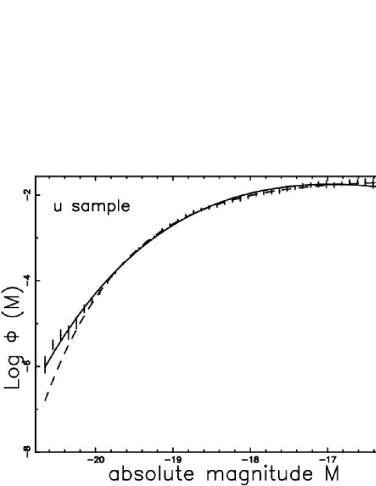
Figure 5: The LF data of SDSS($u^{*}$) are represented through the error bar. The fitting continuous line represents our LF (33) and the dotted line represents the Schechter function.

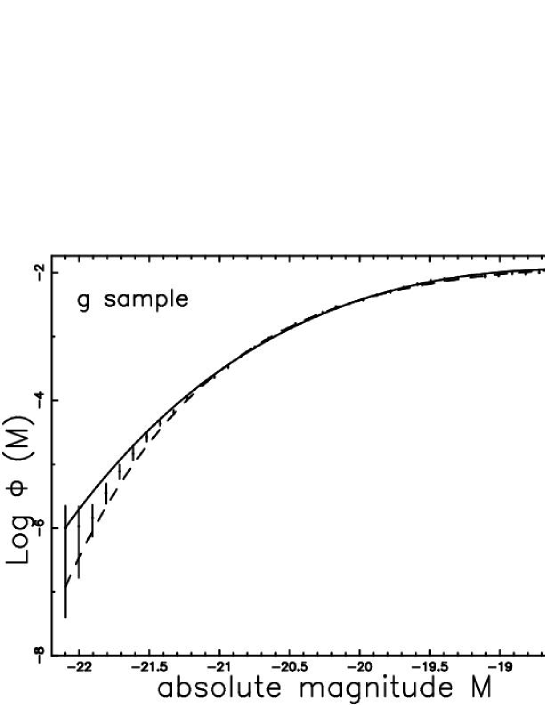
Figure 6: The LF data of SDSS($g^{*}$) are represented through the error bar. The fitting continuous line represents our luminosity function (33) and the dotted line represents the Schechter function.

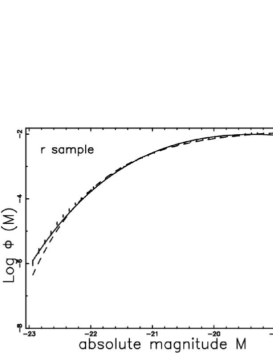
Figure 7: The LF data of SDSS($r^{*}$) are represented through the error bar. The fitting continuous line represents our LF (33) and the dotted line represents the Schechter LF.

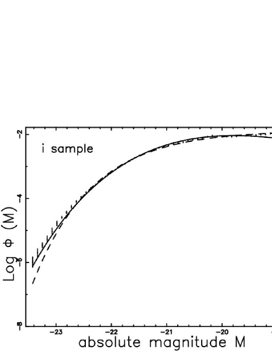
Figure 8: The LF data of SDSS($i^{*}$) are represented through the error bar. The fitting continuous line represents our LF (33) and the dotted line represents the Schechter LF.

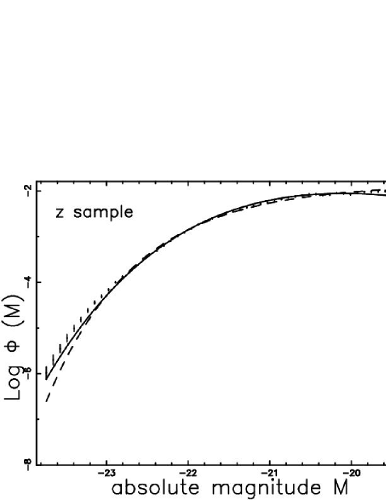
Figure 9: The LF data of SDSS($z^{*}$) are represented through the error bar. The fitting continuous line represents our luminosity function (33) and the dotted line represents the Schechter LF.

4.3 A non linear mass-luminosity relationship

Also here we assume that the mass of the galaxies , ${\mathcal{M}}$, is distributed as $h(\mathcal{M})$. The first transformation is

$$\mathcal{M}=\left(\frac{L}{L^{*}}\right)^{\frac{1}{a}}\quad,$$ (34)

where $L$ is the luminosity , $1/a$ is an exponent that connects the mass to the luminosity and ${L^{*}}$ represents the scale of the luminosity. Equation (12) changes to

$$\Psi^{NL}({L})d{L}=\frac{\Psi^{*}}{a}\,32\,{L}^{-{\frac{-2+a}{a}}}{L^{*}}^{-\frac{2}{a}}{\it K_{0}}\left(4\,{L}^{\frac{1}{2a}}{L^{*}}^{-\frac{1}{2a}}\right)d\frac{L}{L^{*}}\quad,$$ (35)

where $\Psi^{*}$ is a normalization factor and the apex NL stands for nonlinear. The mean luminosity per unit volume, $j$ ,

$$j=\int^{\infty}_{0}L\Psi^{NL}(L)dl={4}^{-a}L^{*}\Psi^{*}\left(\Gamma\left(2+a\right)\right)^{2}\quad.$$ (36)

The second transformation connects the luminosity with the absolute magnitude

$$\Psi^{NL}(M)dM=12.8\,{\it\Psi^{*}}\,{10}^{-0.8\,{\frac{-{\it M^{*}}+{\it M}}{a}}}{\it K_{0}}\left(4.0\,{10}^{-0.2\,{\frac{-{\it M^{*}}+{\it M}}{a}}}\right)\frac{\ln\left(10\right)}{a}dM\quad.$$ (37)

The parameters that should be deduced from the data are $M^{*}$ , $a$ and $\Psi^{*}$. Table 4 reports the original range in magnitude of the astronomical data , the selected range adopted for testing purposes , the three parameter of our function , the $\chi^{2}$ of the fit and the $\chi^{2}$ of the of the Schechter function for the five bands of SDSS. Also here in the $u^{*}$ case the astronomical range and the selected range are coincident.

Table 4: The full range in magnitudes , the selected range in magnitudes , the parameters of our mass-luminosity function (37) , $\chi^{2}$ , $AIC$ and $BIC$ of our mass-luminosity function and the Schechter LF for the SDSS catalog

$$\begin{array}[]{lccccc}\hline\cr parameter&u^{*}&g^{*}&r^{*}&i&z\\ \vskip 3.0pt plus 1.0pt minus 1.0pt\cr\hline\cr\vskip 3.0pt plus 1.0pt minus 1.0pt\cr full~{}range~{}[mags]&-22,-15.8&-23.4,-16.3&-24.48,-16.3&-24.48,-17.2&-23.7,-17.48\\ \vskip 3.0pt plus 1.0pt minus 1.0pt\cr selected~{}range~{}[mags]&-20,-15.78&-22,-18.2&-22.94,-18.5&-23.42,-19.3&-23.7,-20\\ \vskip 3.0pt plus 1.0pt minus 1.0pt\cr a&0.98&0.95&1.07&1.04&1.05\\ \vskip 3.0pt plus 1.0pt minus 1.0pt\cr M^{*}[mags]&-17.27&-18.85&-19.47&-19.98&-20.28\\ \vskip 3.0pt plus 1.0pt minus 1.0pt\cr\Psi^{*}&0.05&0.03&0.033&0.027&0.027\\ \vskip 3.0pt plus 1.0pt minus 1.0pt\cr\chi^{2}&552&803&1180&306&475\\ \vskip 3.0pt plus 1.0pt minus 1.0pt\cr AIC,k=3&558&809&1186&312&481\\ \vskip 3.0pt plus 1.0pt minus 1.0pt\cr BIC,k=3&570&821&1199&325&493\\ \vskip 3.0pt plus 1.0pt minus 1.0pt\cr\chi^{2}~{}Schechter&330&456&1497&1863&2292\\ \vskip 3.0pt plus 1.0pt minus 1.0pt\cr AIC~{}Schechter,k=3&336&462&1503&1869&2298\\ \vskip 3.0pt plus 1.0pt minus 1.0pt\cr BIC~{}Schechter,k=3&349&474&1515&1882&2310\\ \vskip 3.0pt plus 1.0pt minus 1.0pt\cr\hline\cr\hline\cr\end{array}$$

In the absence of observational data which represent the LF , we can generate them through Schechter’s parameters, see Table 2; this is done, for example, for the CFA Redshift Survey ,see [40]. The parameters of the first LF ( equation (33)) are reported in Table 5 where the requested errors on the values of luminosity are the same as the considered value.

Table 5: The parameters of the first LF
based on data from CFA Redshift Survey ( triplets generated by the author)

$$\begin{array}[]{lc}\hline\cr{}&CFA\\ \vskip 3.0pt plus 1.0pt minus 1.0pt\cr\hline\cr\vskip 3.0pt plus 1.0pt minus 1.0pt\cr M^{*}[mags]&-19\pm 0.1\\ \vskip 3.0pt plus 1.0pt minus 1.0pt\cr\Psi^{*}[h~{}Mpc^{-3}]&0.4\pm 0.01\\ \vskip 3.0pt plus 1.0pt minus 1.0pt\cr\hline\cr\hline\cr\end{array}$$

4.4 Parameters determination

The theoretical LF for galaxies can be represented by an analytical function of the type $\Phi(M^{*},\phi^{*},p_{3})$ where $M^{*},\phi^{*}$ and $p_{3}$ represent the scaling magnitude , the number of galaxies per unit $Mpc$ and a generic third parameter. Once the observational data are provided in $n$ triplets made by absolute magnitude , $\phi_{astr}$ ( in units of number per $h^{-3}Mpc^{-3}$ per mag) and $\sigma_{\phi}$ ( the error on $\phi$ ) we can deduce these three parameters in the following ways.

• A scanning on the presumed values of the parameters that are unknown. The three parameters are those that minimize the merit function $\chi^{2}$ computed as

  $$\chi^{2}=\sum_{j=1}^{n}(\frac{\phi-\phi_{astr}}{\sigma_{\phi}})^{2}\quad.$$ (38)

• A nonlinear fit through the Levenberg–Marquardt method ( subroutine MRQMIN in [16]). In this case the first derivative of the LF with respect to the unknown parameters should be provided.

Particular attention should be paid to the number of parameters that are unknown : two for the new LF as represented by formula (33) , three for the Schechter function (formula (26)) and the new mass-LF relationship (formula (37)). The Akaike information criterion ($AIC$) , see [47] , is defined as

$$AIC=2k-2ln(L)\quad,$$ (39)

where $L$ is the likelihood function and $k$ the number of free parameters of the model. We assume a Gaussian distribution for the errors and the likelihood function can be derived from the $\chi^{2}$ statistic $L\propto\exp(-\frac{\chi^{2}}{2})$ where $\chi^{2}$ has been computed trough equation (38), see [48],[49]. Now $AIC$ becomes

$$AIC=2k+\chi^{2}\quad.$$ (40)

The Bayesian information criterion (BIC), see [50], is

$$BIC=k~{}ln(n)-2ln(L)\quad,$$ (41)

where $L$ is the likelihood function , $k$ the number of free parameters of the model and $n$ the number of observations.

4.5 Dependence from the redshift

The joint distribution in z (redshift) and f (flux) for galaxies , see formula (1.104) in [51] or formula (1.117) in [43] , is

$$\frac{dN}{d\Omega dzdf}=4\pi\bigl{(}\frac{c}{H_{0}}\bigr{)}^{5}z^{4}\Psi(\frac{z^{2}}{z_{crit}^{2}})\quad,$$ (42)

where $d\Omega$ , $dz$ and $df$ represent the differential of the solid angle , the redshift and the flux respectively. The critical value of $z$ , $z_{crit}$ , is

$$z_{crit}^{2}=\frac{H_{0}^{2}L^{*}}{4\pi fc_{L}^{2}}\quad.$$ (43)

The number of galaxies , $N_{s}(z,f_{min},f_{max})$ comprised between a minimum value of flux, $f_{min}$, and maximum value of flux $f_{max}$ , can be computed through the following integral

$$N_{S}(z)=\int_{f_{min}}^{f_{max}}4\pi\bigl{(}\frac{c}{H_{0}}\bigr{)}^{5}z^{4}\Psi(\frac{z^{2}}{z_{crit}^{2}})df\quad.$$ (44)

This integral does not have an analytical solution and we performed a numerical integration. The number of galaxies in z and f as given by formula (42) has a maximum at $z=z_{pos-max}$ , where

$$z_{pos-max}=1.3798\times z_{crit}\quad,$$ (45)

that can be re-expressed as

$$z_{pos-max}=\frac{0.3892\,\sqrt{{10}^{0.4\,{\it{\it M_{\hbox{$\odot$}}}}-0.4\,{\it M^{*}}}}{\it H_{0}}}{\sqrt{f}{\it c_{L}}}\quad,$$ (46)

where $M_{\hbox{$\odot$}}$ is the reference magnitude of the sun at the considered bandpass, $H_{0}$ is the Hubble constant and $c_{L}$ is the velocity of the light.

From the point of view of the astronomical observations the second CFA2 redshift Survey , started in 1984, produced slices showing that the spatial distribution of galaxies is not random but distributed on filaments that represent the 2D projection of 3D bubbles. We recall that a slice comprises all the galaxies with magnitude $m_{b}~{}\leq~{}16.5$ in a strip of $6^{\circ}$ wide and about $130^{\circ}$ long. One such slice (the so called first CFA strip) is visible at the following address http://cfa-www.harvard.edu/ huchra/zcat/ and is reported in Figure 10 ; more details can be found in [52].

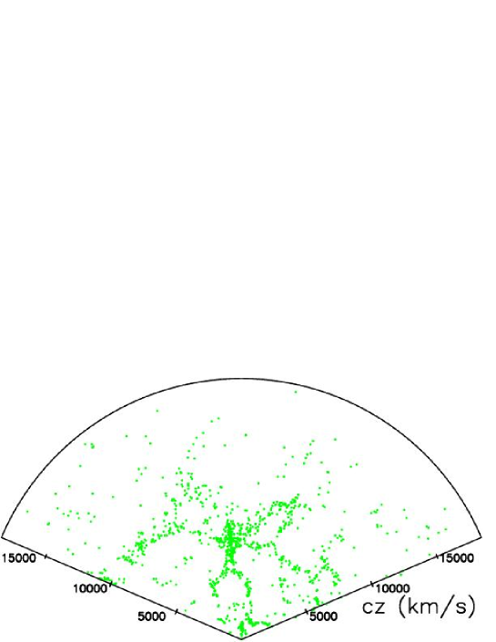
Figure 10: Polar plot of the real galaxies (green points) belonging to the second CFA2 redshift catalogue.

Figure 11 reports the number of observed galaxies of the second CFA2 redshift catalogue for a given magnitude and the theoretical curve as represented by formula (42).

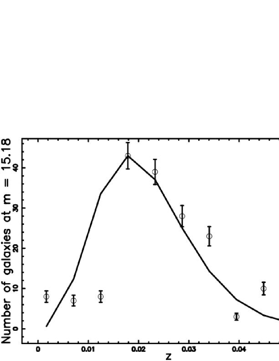
Figure 11: The galaxies of the second CFA2 redshift catalogue with $15.08\leq mag\leq 15.27$ or $48776\frac{L_{\hbox{$\odot$}}}{Mpc^{2}}\leq f\leq 58016\frac{L_{\hbox{$\odot$}}}{Mpc^{2}}$ ( with $mag$ representing the relative magnitude used in object selection), are isolated in order to represent a chosen value of $m$ and then organized in frequencies versus heliocentric redshift , (empty circles); the error bar is given by the square root of the frequency. The maximum in the frequencies of observed galaxies is at $z=0.02$. The theoretical curve generated by the z-dependence in the number of galaxies (formula (42) and parameters as in column CFA of Table 5) is drawn (full line).

The total number of galaxies of the second CFA2 redshift catalogue is reported in Figure 12 as well as the theoretical curve as represented by the numerical integration of formula (44).

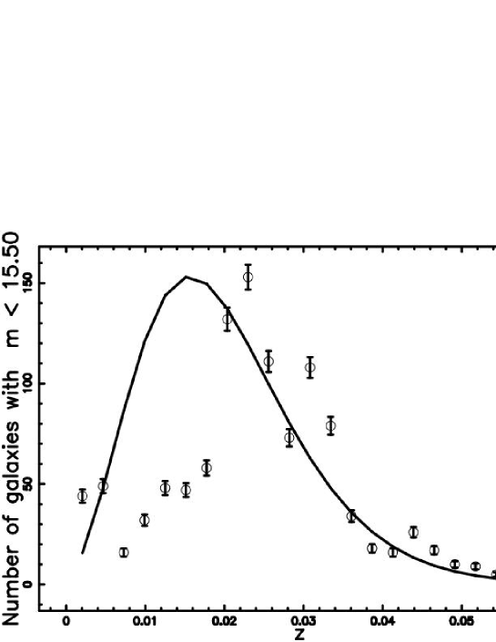
Figure 12: The galaxies of the the second CFA2 redshift catalogue with $10.56\leq mag\leq 15.5$ or $39517\frac{L_{\hbox{$\odot$}}}{Mpc^{2}}\leq f\leq 3739299\frac{L_{\hbox{$\odot$}}}{Mpc^{2}}$ , are organized in frequencies versus redshift , (empty stars). The theoretical curves generated by the integral in flux (formula (44) with parameters as in Table 5) (full line) is drawn.

A typical polar plot is reported in Figure 13 once the number of galaxies as a function of $z$ is computed through the numerical integration of formula (44) ; it should be compared with the observations , see Figure 10.

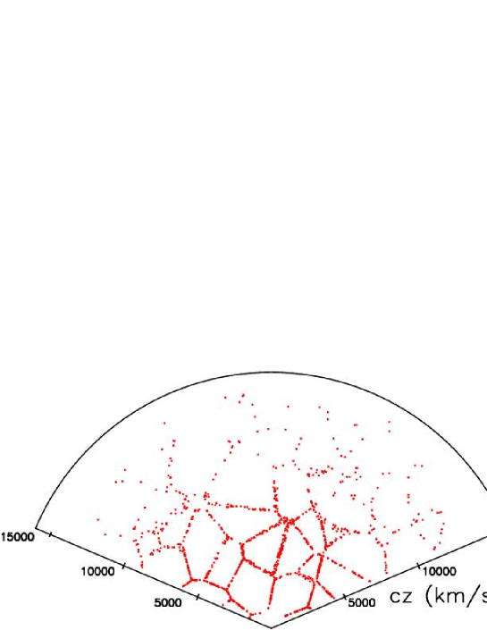
Figure 13: Polar plot of the little cubes (red points) belonging to the simulation. Parameters as in Figure 3.

5 Summary

The PDF of the product of two independent random variables $X$ and $Y$ as represented by two gamma variates with argument 2 has been analytically derived.

The mean , the variance and the DF of this new PDF are computed. As an application we assumed that the mass of the galaxies behaves in the same way as this new PDF. The LF for galaxies can therefore derived assuming a linear or nonlinear relationship between mass and luminosity: in the first case we have a two parameter LF and in the second case a three parameter LF; recall that the Schechter LF for galaxies has three parameters. The parameter $a$ that characterizes the non-linear relationship between mass and luminosity of the second LF , see equation (37) , is found to be around 1.

The comparison between the two LF for galaxies here derived is performed on the SDSS data and can be done only by introducing an upper limit in magnitude , $M_{lim}$, in the five bands analyzed. The three tests of reliability here adopted show that the Schechter function always has a smaller $\chi^{2}$ , $AIC$ and $BIC$ with respect to the two new LF for galaxies here derived , see Table 3 and Table 4.

The theoretical number of galaxies as a function of the red-shift presents a maximum that is a function of $\alpha$ and $f$ for the Schechter function; conversely, when the first new LF here derived is considered , the maximum is a function only of $f$, see equation (45). The first new LF for galaxies , once implemented on a 3D Voronoi slice , allow us to reproduce the large scale structures of our universe.

References

- [1] C. Su, Y. Chen, Science in China Series A-Mathematics 49, 342(2006) .
- [2] J. Salo, H. El-Sallabi, P. Vainikainen, IEEE Transsactions on Antennas and Propagation, 54, 639(2006) .
- [3] T. Kiang, Zeitschrift fur Astrophysics 64, 433(1966) .
- [4] W. Feller, An introduction to probability theory and its applications, Wiley, New York, 1971.
- [5] M. I. Tribelsky, Phys. Rev. Lett. 89 (7), 070201(2002) .
- [6] S. Kumar, S. K. Kurtz, J. R. Banavar, S. M.G., Journal of Statistical Physics 67, 523(1992) .
- [7] L. Zaninetti, Chinese J. Astron. Astrophys.6, 387(2006) .
- [8] M. Tanemura, J. Microscopy 151, 247(1988) .
- [9] M. Tanemura, Forma 18, 221(2003) .
- [10] A. L. Hinde , R. Miles, J. Stat. Comput. Simul. 10, 205(1980) .
- [11] J.-S. Ferenc, Z. Néda, Physica A Statistical Mechanics and its Applications 385, 518(2007) .
- [12] M. P. Silverman, APS Meeting Abstracts , J1005+(2003) .
- [13] A. Glen, J. Leemis, L.M.and Drew, Computational Statistics & Data Analysis 44, 451(2004) .
- [14] M. Springer, The Algebra of Random Variables, Wiley, New York, 1979.
- [15] M. Abramowitz, I. A. Stegun, Handbook of mathematical functions with formulas, graphs, and mathematical tables, Dover, New York, 1965.
- [16] W. H. Press, S. A. Teukolsky, W. T. Vetterling, B. P. Flannery, Numerical recipes in FORTRAN. The art of scientific computing, Cambridge University Press, Cambridge, 1992.
- [17] D. von Seggern, CRC Standard Curves and Surfaces, CRC, New York, 1992.
- [18] W. J. Thompson, Atlas for computing mathematical functions, Wiley-Interscience, New York, 1997.
- [19] G. Voronoi, Z. Reine Angew. Math 133, 97(1907) .
- [20] G. Voronoi, Z. Reine Angew. Math 134, 198(1908) .
- [21] V. Icke, R. van de Weygaert, A&A 184, 16(1987) .
- [22] M. Pierre, A&A 229, 7(1990) .
- [23] J. D. Barrow, P. Coles, MNRAS 244, 188(1990) .
- [24] P. Coles, Nature 349, 288(1991) .
- [25] S. Ikeuchi, E. L. Turner, MNRAS 250, 519(1991) .
- [26] M. Ramella, W. Boschin, D. Fadda, M. Nonino, A&A 368, 776(2001) .
- [27] M. Ramella, M. Nonino, W. Boschin, D. Fadda, Cluster Identification via Voronoi Tesselation, in: G. Giuricin, M. Mezzetti, P. Salucci (Eds.), Observational Cosmology: The Development of Galaxy Systems, Vol. 176 of Astronomical Society of the Pacific Conference Series, 1999, 108–+.
- [28] E. Panko, P. Flin, Astronomical and Astrophysical Transactions 25, 455(2006) .
- [29] E. Panko, P. Flin, Journal of Astronomical Data 12, 1(2006) .
- [30] J. C. Charlton, D. N. Schramm, ApJ 310, 26(1986) .
- [31] L. Zaninetti, M. Ferraro, A&A 239, 1(1990) .
- [32] A. Okabe, B. Boots, K. Sugihara, Spatial tessellations. Concepts and Applications of Voronoi diagrams, Wiley, Chichester, New York, 1992.
- [33] R. L. Bowers, T. Deeming, Astrophysics. I and II, Jones and Bartlett , Boston, 1984.
- [34] P. Schechter, ApJ 203, 297(1976) .
- [35] T. Kiang, MNRAS 122, 263(1961) .
- [36] G. Efstathiou, R. S. Ellis, B. A. Peterson, MNRAS 232, 431(1988) .
- [37] N. Cross, S. P. Driver, W. Couch, C. M. Baugh, J. Bland-Hawthorn, T. Bridges, R. Cannon, S. Cole, M. Colless, C. Collins, G. Dalton, K. Deeley, R. De Propris, G. Efstathiou, R. S. Ellis, C. S. Frenk, K. Glazebrook, C. Jackson, O. Lahav, I. Lewis, S. Lumsden, S. Maddox, D. Madgwick, S. Moody, P. Norberg, J. A. Peacock, B. A. Peterson, I. Price, M. Seaborne, W. Sutherland, H. Tadros, K. Taylor, MNRAS 324, 825(2001) .
- [38] M. R. Blanton, J. Dalcanton, D. Eisenstein, J. Loveday, M. A. Strauss, M. SubbaRao, D. H. Weinberg, J. E. Anderson, J. Annis, N. A. Bahcall, M. Bernardi, J. Brinkmann, R. J. Brunner, AJ121, 2358(2001) .
- [39] S. P. Driver, J. Liske, N. J. G. Cross, R. De Propris, P. D. Allen, MNRAS 360, 81(2005) .
- [40] R. O. Marzke, J. P. Huchra, M. J. Geller, ApJ 428, 43(1994) .
- [41] S. P. Driver, S. Phillipps, ApJ 469, 529(1996) .
- [42] M. R. Blanton, R. H. Lupton, D. J. Schlegel, M. A. Strauss, J. Brinkmann, M. Fukugita, J. Loveday, ApJ 631, 208(2005) .
- [43] P. Padmanabhan, Theoretical astrophysics. Vol. III: Galaxies and Cosmology, Cambridge University Press, Cambridge, MA, 2002.
- [44] A. N. Cox, Allen’s astrophysical quantities, Springer, New York, 2000.
- [45] H. Lin, R. P. Kirshner, S. A. Shectman, S. D. Landy, A. Oemler, D. L. Tucker, P. L. Schechter, ApJ 464, 60(1996) .
- [46] J. Machalski, W. Godlowski, A&A 360, 463(2000) .
- [47] H. Akaike, IEEE Transactions on Automatic Control 19, 716(1974) .
- [48] A. R. Liddle, MNRAS 351, L49(2004) .
- [49] W. Godlowski, M. Szydowski, Constraints on Dark Energy Models from Supernovae, in: M. Turatto, S. Benetti, L. Zampieri, W. Shea (Eds.), 1604-2004: Supernovae as Cosmological Lighthouses, Vol. 342 of Astronomical Society of the Pacific Conference Series, 2005, 508–+.
- [50] G. Schwarz, Annals of Statistics 6, 461(1978) .
- [51] T. Padmanabhan, Cosmology and Astrophysics through Problems, Cambridge University Press, Cambridge, 1996.
- [52] M. J. Geller, J. P. Huchra, Science 246, 897(1989) .