Confirming and extending the hypothesis of universality in sandpiles

Abstract

Stochastic sandpiles self-organize to a critical point with scaling behavior different from directed percolation (DP) and characterized by the presence of an additional conservation law. This is usually called C-DP or Manna universality class. There remains, however, an exception to this universality principle: a sandpile automaton introduced by Maslov and Zhang, which was claimed to be in the directed percolation class despite of the existence of a conservation law. In this paper we show, by means of careful numerical simulations as well as by constructing and analyzing a field theory, that (contrarily to what previously thought) this sandpile is also in the C-DP or Manna class. This confirms the hypothesis of universality for stochastic sandpiles, and gives rise to a fully coherent picture of self-organized criticality in systems with a conservation law. In passing, we obtain a number of results for the C-DP class and introduce a new strategy to easily discriminate between DP and C-DP scaling.

I Introduction

Aimed at shedding some light on the origin of scale invariance in many contexts in Nature, different mechanisms for self-organized criticality (SOC) were proposed during the last two decades following the seminal work by Per Bak and coauthors BTW ; Dhar ; Sandpiles . Sandpiles, ricepiles, and earthquake toy-models become paradigmatic examples capturing the essence of self-organization to scale-invariant (critical) behavior without apparently requiring the fine tuning of parameters (see GG ; SOC ; VZ ).

Sandpiles played a central role in the development of this field BTW ; Dhar ; Sandpiles . They are metaphors of real systems (as earthquakes, snow avalanches, stick-slip phenomena, etc.) in which some type of stress or energy is accumulated at some slow timescale and relaxed in a much faster way. In sandpiles, grains are slowly added and eventually relaxed whenever a local instability threshold is overcome; then they are transmitted to neighboring sites which, on their turn, may become unstable and relax, generating avalanches of activity. Considering open boundaries to allow for an energy balance, a steady state with power-law distributed avalanches is eventually reached.

In order to rationalize sandpiles in particular, and SOC in general, and to understand their critical properties, it was proposed DVZ ; FES ; BJP to look at them as systems with many absorbing states AS ; many . The underlying idea is that, in the absence of external driving, sandpile models get eventually trapped into stable configurations from which they cannot escape, i.e. absorbing states AS . The concept of fixed energy sandpiles (FES) was introduced to make this connection more explicit. FES sandpiles share the microscopic rules with their standard (slowly driven and dissipative) counterparts, but with no driving nor dissipation. In this way, the total amount of sand or energy becomes a conserved quantity acting as a control parameter. Calling $E_{c}$ the average density of energy of a standard sandpile in its stationary (self-organized) critical state, it has been shown that the corresponding fixed-energy sandpile exhibits a transition from an active phase to an absorbing one at, precisely, $E_{c}$. It can be argued that slow driving and dissipation acting together at infinitely separated time-scales constitute a mechanism able to pin a generic system with absorbing states and a conservation law to its critical point GG ; VZ ; DVZ ; FES ; BJP ; abs_others .

Using the relation with transitions into absorbing states interfaces , a Langevin equation describing FES stochastic sandpiles was proposed BJP ; FES in the spirit of Hohenberg and Halperin HH . The Langevin equation is similar to the well known directed-percolation (DP) Langevin equation describing generic systems with absorbing states conjecture ; AS but, additionally, it is coupled linearly to a conserved non-diffusive energy field, representing the conservation of energy grains in the sandpile dynamics FES ; BJP :

$$\displaystyle{\partial_{t}\rho(x,t)} = a\rho-b\rho^{2}+\omega\rho E(x,t)+\nabla^{2}\rho+\sigma\sqrt{\rho}\eta(x,t)$$

$$\displaystyle{\partial_{t}E(x,t)} = D\nabla^{2}\rho,$$ (1)

where $D$, $a$, $b$ and $\omega$ are constants, $\rho(x,t)$ and $E(x,t)$ are the activity and the energy field, respectively, while $\eta$ is a zero-mean Gaussian white noise. The universality class described by this Langevin equation, which includes sandpiles as well as all other systems with many absorbing states and a non-diffusive conserved field, is usually called Manna or C-DP class Rossi ; FES ; BJP ; note . As a side note, let us remark that the original Bak-Tang-Wiesenfeld model, being deterministic, has many other conservation laws (toppling invariants) and is therefore not described by the present stochastic theory deter1 ; BJP .

Incidentally, even if it has been clearly established that DP and C-DP constitute two different universality classes Romu ; Lubeck ; DCM , most of their universal features (critical exponents, moment ratios, scaling functions,…) are very similar, making it difficult to discriminate numerically between both classes in any spatial dimension.

Despite of the fact that the critical behavior of stochastic sandpiles is accepted to be universal and described by Eq.(1), there are a few sandpile models which, despite of being conservative, have been argued to exhibit a different type of critical behavior MD ; MZ , namely DP, violating the conjecture of universality:

• the Mohanty-Dhar (MD) sandpile MD , in which grains have some probability to remain stable even if they are above the instability threshold. It was argued, based on numerical simulations and on exact results for an anisotropic version of it, that the (isotropic) MD sandpile should exhibit DP-like behavior MD

• the Maslov and Zhang (MZ) sandpile MZ , in which not only the grains of unstable sites are redistributed among nearest neighbors. Instead, all the grains in the local neighborhood of unstable sites are randomly redistributed or reshuffled. On the basis of Monte Carlo simulations this sandpile was argued to exhibit DP behavior.

Aimed at clarifying this puzzling situation, in a recent work we provided strong numerical and analytical evidence that, contrarily to what previously thought, the (isotropic) MD sandpile is actually in the C-DP class Rapid ; Jabo2 (see MD2 for a discrepant viewpoint). To further substantiate our claim, in Jabo2 we proposed a strategy to easily discriminate between DP and C-DP consisting in introducing a wall (either absorbing or reflecting); systems in the DP and in the C-DP classes behave in (qualitative and quantitatively) very different ways in the presence of walls, providing an easy criterion to discriminate between both classes.

Our goal in the present paper is to scrutinize the last remaining piece in the puzzle, i.e. the MZ model, by employing extensive numerical simulations as well as field theoretical considerations. For the numerics, we take advantage of the previously introduced discrimination criterion and, also, present another method to easily discriminate between DP and C-DP, based in the introduction of anisotropy in one spatial direction.

The analyses presented on what follows, show in a clean-cut way that the MZ model is actually in the C-DP class. This leaves no dangling end in the sandpile universality picture and, as a byproduct, confirms the general validity of the absorbing-state approach to rationalize SOC. New results for the C-DP class are also obtained.

II The Maslov-Zhang sandpile

The Maslov-Zhang (MZ) sandpile MZ is defined as follows:

1. Driving: an input energy, $\delta E\leq 1$, is added to the central (or to a randomly chosen) site, $i$, of a d-dimensional lattice, and the site is declared active.

2. Relaxation: energy is locally redistributed (“reshuffled”) between the active site and its nearest-neighbors, according to:

   $$E_{i}=\frac{r_{i}}{\sum_{j=1}^{2d+1}r_{j}}\displaystyle\sum_{j=1}^{2d+1}E_{j},$$ (2)

   where $r_{i}$ are uniformly distributed ($r_{i}\in\left[0,1\right]$) random variables, and the sums are performed over the site $i$ and its $2d$ nearest neighbors.

3. Activation: each of the sites involved in the reshuffling is declared active with a probability given by its own energy, triggering the generation of avalanches of activity.

4. Avalanches: new active sites are added to a list and relaxed in a sequential way.

5. Dissipation: energy arriving at the open borders is removed from the system.

6. Avalanches proceed until all activity ceases, and then a new external input is added. Eventually a critical stationary state is reached.

Monte Carlo simulations by Maslov and Zhang revealed exponents compatible with those of directed percolation in two dimensions and above, while in one dimension some anomalies in the scaling were reported MZ . Later, simulations of the FES counterpart of the MZ sandpile led to very similar results FES .

Before entering a more careful numerical analysis of the MZ sandpile, we take a detour to construct explicitely a Langevin equation for such a model. This will allow us to better understand what the main relevant ingredients of the MZ model are and in what sense it differs from other C-DP models and from Eq.(1).

III A Langevin Equation for the Maslov-Zhang sandpile

The main difference between the Maslov-Zhang cellular automaton and other sandpiles in the C-DP universality class is that, while in the C-DP class as the Manna model, the only energy redistributed by the dynamics (by topplings) is that accumulated in active sites, in the MZ dynamics both the energy of active sites as well as that of its nearest neighbors is redistributed. This leads to a more severe local redistribution of energy, that we quantify in what follows in terms of a new set of Langevin equations, first in a phenomenological way and then by deriving it from the microscopic rules.

III.1 Phenomenological Langevin equation

Diffusion of energy occurs in the C-DP class by means of activity relaxation. At a mesoscopic level, this implies that the rate of change of the energy density $E(x,t)$ at a given position is proportional to minus the divergence of a current, $\partial_{t}E(x,t)=-\nabla.j(x,t)$, where $j(x,t)$ is given by the gradient of the activity field,

$$j(x,t)=-D~{}\nabla\rho(x,t)$$ (3)

leading to $\partial_{t}E(x,t)=D\nabla^{2}\rho(x,t)$ in Eq.(1).

Instead, in the MZ model, changes of energy are controlled by the reshuffling rule, i.e. energy does not need to be at an active site (but in its neighborhood) to be redistributed. Hence, at a mesoscopic level the current is given by gradients of the energy in the presence of non-vanishing activity. More specifically, $\partial_{t}E(x,t)=-\nabla.j(x,t)$ where now

$$j(x,t)=-\tilde{D}~{}\nabla E(x,t),$$ (4)

and the diffusion $\tilde{D}$ is not a constant but a functional proportional to $\rho(x,t)$, $\tilde{D}(\rho(x,t))=D\rho(x,t)$ capturing the requirement that local reshuffling of energy only occurs in the presence of activity. This enforces the absorbing state condition that dynamics ceases if $\rho=0$. This finally leads to

$$\partial_{t}E(x,t)=D~{}\nabla.[\rho(x,t)\nabla E(x,t)].$$ (5)

On the other hand, the equation for the activity is not expected to change in any relevant way, so one obtains

$$\displaystyle{\partial_{t}\rho(x,t)} = a\rho-b\rho^{2}+\nabla^{2}\rho+\omega\rho E(x,t)+\sigma\sqrt{\rho}\eta(x,t)$$

$$\displaystyle{\partial_{t}E(x,t)} = D\nabla.[\rho(x,t)\nabla E(x,t)]$$ (6)

representing the MZ dynamics at a mesoscopic level. This is to be compared with Eq.(1).

III.2 Microscopic derivation of the Langevin equation

To gain more confidence on the phenomenological set of equations, Eq. (6) let us now present an explicit microscopic derivation. We consider a parallel version of the MZ model in which all active sites are relaxed at every time step. To do so, we assume that each site uses a fraction $1/(2d+1)$ of its total energy for eventual redistributions with each of the sites in its local neighborhood. At mean-field level, the energy evolves according to

$$\begin{array}[]{rl}E_{i,t+1}=&\dfrac{1}{2d+1}E_{i,t}\displaystyle\sum_{j=1}^{2d+1}\left[1-\Theta(\rho_{j,t})\right]\\ +&\dfrac{1}{2d+1}\displaystyle\sum_{j=1}^{2d+1}\Theta(\rho_{j,t})\sum_{k=1}^{2d+1}\dfrac{E_{k,t}}{2d+1}\end{array}$$ (7)

where $j$ (respectively $k$) runs over the nearest neighbors of $i$ ($j$) and $\Theta$ is the Heaviside step function ($\Theta(z)=0$ if $z\leq 0$). For any inactive site in the local neighborhood (i.e. $\rho_{j}=0$), the central site does not redistribute the corresponding fraction of its energy (first term in Eq.(7)). For any active site in the local neighborhood (i.e. $\rho_{j}>0$) the central site receives on average a corresponding fraction of energy (second term). Eq.(7) is a mean-field equation to which fluctuations should be added to have a more detailed description. Such fluctuations appear as a (conserved) noise for the resulting energy equation and can be easily argued to constitute a higher order, irrelevant, correction.

Regularizing the Heaviside step function in Eq.(7) by means of a hyperbolic-tangent and expanding it in power series up to first order in $\rho$ Rapid , we obtain

$$\begin{array}[]{rl}E_{i,t+1}=&\dfrac{1}{2d+1}E_{i,t}\displaystyle\sum_{j=1}^{2d+1}\left[1-\rho_{j,t}\right]\\ +&\dfrac{1}{2d+1}\displaystyle\sum_{j=1}^{2d+1}\rho_{j,t}\sum_{k=1}^{2d+1}\dfrac{E_{k,t}}{2d+1}.\end{array}$$ (8)

Introducing the $d$-dimensional discrete Laplacian $\nabla^{2}E_{i}=\sum_{j=1}^{2d}(E_{j}-E_{i})$ the first term can be rewritten as:

$$\begin{array}[]{rl}\dfrac{E_{i}}{2d+1}\displaystyle\sum_{j=1}^{2d+1}\left[1-\rho_{j}\right]=&E_{i}-\dfrac{E_{i}}{2d+1}\displaystyle\sum_{j=1}^{2d+1}\rho_{j}\\ =&E_{i}-E_{i}\rho_{i}-\dfrac{E_{i}}{2d+1}\nabla^{2}\rho_{i}.\end{array}$$ (9)

Similarly, the second term can be expressed as

$$\begin{array}[]{rl}\dfrac{1}{(2d+1)^{2}}\displaystyle\sum_{j=1}^{2d+1}\rho_{j}\left(\displaystyle\sum_{k=1}^{2d+1}E_{k}\right)=&E_{i}\rho_{i}+\dfrac{1}{(2d+1)}\nabla^{2}\left(E_{i}\rho_{i}\right)\\ +\dfrac{1}{(2d+1)}\rho_{i}\nabla^{2}E_{i}+&\dfrac{1}{(2d+1)^{2}}\nabla^{2}\left(\rho_{i}\nabla^{2}E_{i}\right).\end{array}$$ (10)

Putting these two contributions together and reorganizing the discrete derivatives, one obtains:

$$\begin{array}[]{ll}&E_{i,t+1}=E_{i,t}+\dfrac{2}{2d+1}\rho_{i,t}\nabla^{2}E_{i,t}+\dfrac{2}{2d+1}\nabla\rho_{i,t}~{}.\nabla E_{i,t}\\ &+~{}\dfrac{1}{(2d+1)^{2}}\nabla^{2}\left(\rho_{i,t}\nabla^{2}E_{i,t}\right)=\\ &E_{i,t}+\dfrac{2}{2d+1}\nabla.\left(\rho_{i,t}\nabla E_{i,t}\right)+\dfrac{1}{(2d+1)^{2}}\nabla^{2}\left(\rho_{i,t}\nabla^{2}E_{i,t}\right)\end{array}$$ (11)

which in the continuous time limit becomes

$$\partial_{t}E_{i}=\dfrac{2}{2d+1}\nabla.\left(\rho_{i,t}\nabla E_{i,t}\right)+\dfrac{1}{(2d+1)^{2}}\nabla^{2}\left(\rho_{i,t}\nabla^{2}E_{i,t}\right).$$ (12)

The second term in this last equation can be argued to be naïvely irrelevant in the renormalization group sense (as it includes higher order derivatives) and hence dropped out. Identifying $D$ with $2/(2d+1)$ we recover the phenomenological Eq.(5), as the leading contribution.

As said above, this is to be compared with the standard Langevin Eq.(1) for the C-DP class, in which the flux of energy is given by the gradient of the activity itself. The following questions pop up naturally: Does Eq. (6) lead to a critical behavior different from that of Eq.(1)? Could this be the reason why the MZ sandpile was claimed to differ from the C-DP class? Is this new form of conserved energy dynamics irrelevant at the DP fixed point, supporting the MZ sandpile to be DP like?

To properly answer these questions one should resort to a full renormalization group calculation. Given that even for the C-DP class this has proven to be a, still not satisfactorily accomplished, difficult task Fred , we will leave aside such a strategy here. Instead, in section IV we will give an answer to these question by means of computational studies of the microscopic MZ model as well as of its equivalent Langevin Eq.(6).

III.3 Naïve power counting

A power counting analysis is not helpful in elucidating the relevancy of the energy-diffusion term, Eq.(5). Actually, as there is a lineal dependence on the energy field in both the r.h.s. and the l.h.s. of Eq.(1), there is no way to extract the energy field naïve dimension nor, hence, to make any statement about the relevancy of the coupling term $w\rho(x,t)E(x,t)$ at the DP fixed point.

On the other hand, it is easy to cast Eq.(6) into a generating functional following standard procedures, to set the basis of a perturbative expansion. However, one soon realizes that technical difficulties similar to those encountered for the analysis of Eq.(6) (including the presence of generically singular propagators Fred ; FES ) show up, hindering the perturbative calculation. It is our believe that some type of non-perturbative technique, or non-conventional perturbative expansion, is required to elucidate the renormalization group fixed point of this type of problems.

The analytical understanding, at a field theory level of C-DP as well as the MZ-Langevin equation remain open challenging tasks.

IV Monte Carlo simulations of the Maslov-Zhang sandpile

We have performed extensive Monte Carlo simulations of the MZ sandpile (and variations of it) and scrutinized its asymptotic (long time and large system size) properties. We report on two different types of numerical experiments.

• “SOC” or avalanche experiments:

  By iterating slow addition of grains in the sandpile with open boundaries, the system self-organizes to a state with average energy $E_{c}$. Then, the avalanche size distribution, $P(s)$ and the avalanche time distribution $P_{t}(t)$, can be estimated and their corresponding exponents, $\tau$ and $\tau_{t}$ avalanches , measured.

• Absorbing state experiments:

  At the stationary state, we perform spreading experiments from a localized seed, and we measure: i) the mean quadratic distance to the initial seed $R^{2}\sim t^{z_{spr}}$ in active runs, ii) the average number of active sites as a function of time, $N(t)\sim t^{\eta}$ and iii) the surviving probability up to time $t$, $P_{s}\sim t^{-\delta}$. We also study the decay at criticality of a homogeneous initial activity ($\rho(t)\sim t^{-\theta}$) in the fixed energy case AS ; avalanches .

Scaling laws relating avalanche to spreading exponents where described systematically in avalanches ; two of them are: $\tau~{}=(1+\eta+2\delta)/(1+\eta+\delta)$, $\tau_{t}~{}=1+\delta$. We measure the exponents independently and use scaling laws as a check for consistency.

We simulate the MZ automaton in one-dimensional lattices up to size $L=2^{15}$. The stationary critical energy density is $E_{c}=0.4928(2)$ and, contrarily to what reported in MZ , we do observe clean scaling at criticality, even if it emerges only after significatively long transients (results not shown) justifying why smaller scale simulations can lead to erroneous conclusions.

The resulting critical exponents are gathered together in Table 1. They are closer in all cases to the C-DP values than to DP ones. Still, given the similarity between the numerical values in both classes, it is not save to extract a definitive conclusion from these results. Higher numerical precision would be required to produce fully convincing evidence.

${\bf d=1}$	$\eta$	$\delta$	$\tau$	$\tau_{t}$	$z_{spr}$	$\theta$
DP	$0.313(1)$	$0.159(1)$	$1.108(1)$	$1.159(1)$	$1.265(1)$	$0.159(1)$
C-DP	$0.350(5)$	$0.170(5)$	$1.11(2)$	$1.17(2)$	$1.39(1)$	$0.125(1)$
MZ	$0.32(5)$	$0.20(5)$	$1.13(5)$	$1.20(5)$	$1.40(5)$	$0.13(1)$

Table 1: Critical exponents for DP, C-DP, and the MZ sandpile in one dimension. DP and C-DP values taken from avalanches ; Lubeck ; Jabo2 .

As said above, the numerical values of DP and C-DP exponents are closer and closer as the dimensionality is increased (they coincide above $d_{c}=4$). Therefore, performing numerical simulations, as the ones above, to discriminate between both classes by using larger and larger times and system sizes in $d\geq 2$ , is not a clever idea. Instead, it is advisable to use/devise more effective numerical strategies to discriminate between DP and C-DP in a simple, efficient, and numerically inexpensive way. For this we use:

• the method devised in Jabo2 consisting in analyzing how the system responds to the presence of a wall, or

• a new strategy, which exploits the fact that systems in these two classes react in remarkably different ways to the introduction of anisotropy in space.

Both of these strategies allow to obtain clean-cut results, as shown in the forthcoming two subsections.

IV.1 Boundary Driven Experiments

The influence of walls in systems in the DP class has been profusely analyzed in the literature DP_wall . In particular, it is well known that, if spreading (and SOC) experiments are performed nearby a wall, the surviving probability is significatively affected, and avalanche and spreading exponents change in a non-trivial way with respect to their bulk counterparts DP_wall . It is also known that in the DP class, both reflecting and absorbing walls lead to a common type of universal “surface critical behavior”, that we call surface directed percolation (SDP), characterized (in one-dimension) by the exponents shown in Table II.

In contrast, the effect of walls in C-DP systems has been studied only recently Jabo2 . Contrarily to the DP case, absorbing and reflecting walls induce different types of surface critical behavior. As illustrated in Table II, all spreading and avalanche exponents take distinct values for an absorbing and for a reflecting wall. Furthermore, the numerical differences between the exponents for either type of wall with respect to their corresponding SDP counterparts are very large, allowing for easy numerical discrimination Jabo2 . Finally, in the C-DP class, the exponents in the presence of a reflecting wall coincide with their bulk counterparts Jabo2 . These features imply that, by introducing a wall in a given system with absorbing states, it becomes straightforward to distinguish if it is in the DP or in the C-DP class, with moderate computational cost.

Following this strategy, we simulated the one-dimensional MZ sandpile, as defined above, in the presence of both reflecting and absorbing walls. In both cases a wall is introduced at the origin (position $i=0$), and the sandpile is studied in the positive half lattice. In the reflecting case, the energy that should go after reshuffling, to the leftmost site, at $i=0$, (whose energy is fixed to zero) is instead added to its closest nearest neighbor to the right, $i=1$. On the other hand, the absorbing condition is imposed by fixing the energy of the leftmost site to zero after every iteration of the microscopic sandpile rules, i.e. by removing from the system at every iteration all the energy received by the leftmost site.

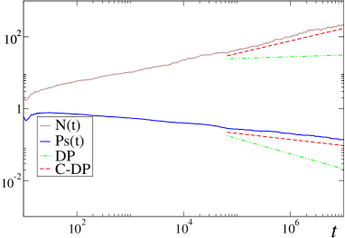
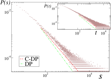
Figure 1: Avalanche exponents for the one-dimensional MZ sandpile in the presence of a reflecting wall. Up: spreading experiments; $N(t)$ is the total number of active sites and $P_{s}(t)$ is the surviving probability; system size $L=2^{15}$ number of runs $500$ . Down: avalanche size (main plot) and time (inset) distributions; system size $L=2^{12}$ number of runs $10^{5}$ . Green (red) lines mark DP (C-DP) scaling (see numerical values in Table 2).

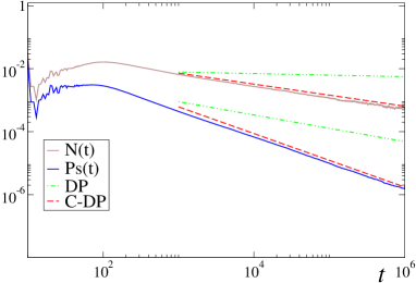
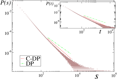
Figure 2: As in Fig. 1 but for an absorbing wall (numerical values summarized in Table 2). System size $L=2^{15}$ and $8\dot{1}0^{7}$ runs.

${\bf d=1}$	$\eta$	$\delta$	$\tau$	$\tau_{t}$	$z_{spr}$	$\theta$
DPref	$0.046(2)$	$0.425(2)$	$1.25(3)$	$1.43(3)$	$1.257(2)$	$0.154(3)$
DPabs	$0.045(2)$	$0.426(2)$	$1.28(3)$	$1.426(2)$	$1.276(2)$	$0.165(2)$
C-DPref	$0.35(1)$	$0.16(1)$	$1.11(2)$	$1.15(2)$	$1.41(1)$	$0.12(1)$
C-DPabs	$-0.33(2)$	$0.85(2)$	$1.56(2)$	$1.81(2)$	$1.43(2)$	$0.13(1)$
MZref	$0.37(5)$	$0.15(5)$	$1.09(5)$	$1.14(5)$	$1.30(5)$	$-$
MZabs	$-0.36(5)$	$0.84(5)$	$1.57(5)$	$1.84(5)$	$1.25(5)$	$-$

Table 2: One-dimensional critical exponents for DP and C-DP without walls avalanches ; Lubeck and in the presence of absorbing and reflecting walls Jabo2 . Values in rows $1$ (DP_ref) and $2$ (DP_abs) coincide within error-bars. Note also, that values in row $3$ ( C-DP_ref ) coincide with those for C-DP (table 1). Results for the MZ sandpile in the presence of reflecting/absorbing walls are reported in the last two rows. $theta$ has not been measured in these cases.

Fig.(1) and Fig.(2) show the results of simulations performed in lattices of system size $L=2^{15}$, averaging over up to $8\dot{1}0^{7}$ runs. The corresponding exponents are summarized in Table II. All of them coincide within numerical accuracy with the expected values for the C-DP class in the presence of reflecting or absorbing walls respectively, and differ significatively from those of SDP. For example, in the presence of a reflecting (respectively, absorbing) wall, the measured value of $\eta$ is $0.37$ ($-0.37$) in good agreement with the C-DP expectation, $\eta=0.35$ ($-0.33$) and in blatant disagreement with the corresponding DP value, $\eta\approx 0.046$ ($\approx 0.045$), which is one order of magnitude smaller (and of opposite sign in the case of an absorbing wall). Similar large differences are measured for all the exponents (see table II). Note also that, as is the case in the C-DP class Jabo2 , the exponents in the presence of a reflecting wall coincide within error-bars with their bulk counterparts. In conclusion, studying the influence of walls we conclude that the one-dimensional MZ sandpile exhibits C-DP scaling.

IV.2 Anisotropic Experiments

It is well known that systems in the DP class are invariant under Galilean transformations: if particles have a tendency to move anisotropically in one preferred spatial direction, that does not alter the critical properties AS . The presence of any degree of anisotropy in DP-like systems is an irrelevant trait, or in other words, anisotropic DP (A-DP) is just DP.

The role of anisotropy in sandpiles has also been profusely studied after the pioneering exact solution by Dhar and Ramaswamy DR of the totally anisotropic or “directed” counterpart of the Bak-Tang-Wiesenfeld sandpile. Anisotropic stochastic sandpiles have also been studied using general principles ani_general and through interfacial representations ani_inter . The conclusion is that all anisotropic sandpiles, as long as they are stochastic deterministic , belong to the same universality class, that we call anisotropic C-DP (A-C-DP) ani_PSV . The critical exponents of models in this class, where first measured numerically ani_PSV , and then exactly calculated in any dimension ani_solution (see table 3 and table 4).

${\bf d=1}$	$\eta$	$\delta$	$\tau$	$\tau_{t}$	$z_{spr}$
DP	$0.33(2)$	$0.14(2)$	$1.09(3)$	$1.14(3)$	$2.00(2)$
A-C-DP	$0$	$1/2$	$4/3$	$3/2$	$2$
A-MZ	$-0.02(3)$	$0.51(3)$	$1.35(5)$	$1.48(5)$	$1.98(3)$

Table 3: One dimensional critical exponents for DP avalanches ; Lubeck , C-DP with a preferred direction (analytical results from ani_solution ), and the anisotropic MZ model.

${\bf d=2}$	$\eta$	$\delta$	$\tau$	$\tau_{t}$	$z_{spr}$
DP	$0.230(1)$	$0.451(1)$	$1.268(1)$	$1.451(1)$	$1.13(2)$
A-C-DP	$0$	$3/4$	$10/7$	$7/4$	$2$
A-MZ	$-0.07(5)$	$0.75(5)$	$1.49(5)$	$1.70(5)$	$1.93(5)$

Table 4: Two-dimensional critical exponents for anisotropic models: A-DP (i.e. DP), A-C-DP (analytical results), and anisotropic-MZ.

The strategy to be used is straightforward: take the MZ sandpile model and switch on anisotropy; if the isotropic model was in the DP class, anisotropy should be an irrelevant ingredient and the anisotropic counterpart should also be DP like. If, instead, the isotropic model is in the C-DP class, then anisotropy is a relevant ingredient and critical exponent change from C-DP to A-C-DP values.

The simplest way to define an anisotropic MZ (A-MZ) model is by fixing one of the $r_{j}$ in Eq.(2), say the one to the right, to its maximum possible value, $r_{j}=1$, and letting the others $r_{j}$ to take randomly distributed values in $\left[0,1\right]$. This generates an overall energy flow towards the preferred direction (to the right, in this case). Anisotropy can be introduced in other ways, including full-anisotropy or directness, but this does not affect our conclusions in any significant way.

Fig. 3 and table 3 show our main results for the one-dimensional MZ model with anisotropy. Both avalanche and spreading exponents are very different from their isotropic counterparts. They also differ notoriously from DP values, but coincide within error-bars with the expected values for the A-C-DP class.

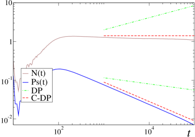
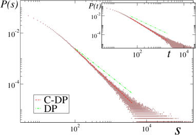
Figure 3: Avalanche exponents for the anisotropic MZ sandpile model in one dimension, averaged over $8\dot{1}0^{6}$ runs (system size $L=2^{18}$). Up: spreading experiments (see Table 3). Down: avalanche size (main plot) and time (inset) distributions. Green lines mark DP scaling while red ones correspond to C-DP scaling.

The same conclusion holds in two dimensions (see Table 4). In this way, as the anisotropic MZ model belongs to A-C-DP class the original, isotropic, MZ sandpile model can be safely concluded to be in the C-DP universality class, confirming the result above.

V Numerical integration of the MZ Langevin equation

In this section we verify that Langevin Eq.(6) is a sound description of the MZ model and that, despite of its different form, it behaves asymptotically as Eq.(1). For that we perform numerical analysis (again, both SOC and absorbing state experiments) using Eq.(6). A direct integration of Eq.(6) in one-dimension, using the recently introduced integration scheme for Langevin equations with square-root noise DCM , produces the exponents reported in the first row of Table 5 (plots not shown). All of them are compatible with those of the microscopic MZ model and the C-DP class (see Table 1).

${\bf d=1}$	$\eta$	$\delta$	$\tau$	$\tau_{t}$	$z_{spr}$	$\theta$
Eq.(6)	$0.28(5)$	$0.21(5)$	$1.14(5)$	$1.21(5)$	$1.25(5)$	$0.14(2)$
Eq.(6)ref	$0.36(5)$	$0.18(5)$	$1.12(5)$	$1.18(5)$	$1.29(5)$	$0.11(5)$
Eq.(6)abs	$-0.39(5)$	$0.85(5)$	$1.58(5)$	$1.85(5)$	$1.22(5)$	$0.15(5)$
Eq.(6)anis	$-0.01(2)$	$0.50(2)$	$1.39(5)$	$1.64(5)$	$1.98(2)$	$0.51(2)$

Table 5: Critical exponents for Eq.(6), with a reflective wall, Eq.(6) with an absorbing wall, and Eq.(6) with an anisotropic term.

Changing the boundary conditions during the integration we implement the reflecting or the absorbing wall. For the former, we impose $\rho(-x,t)=\rho(x,t),~{}~{}E(-x,t)=E(x,t),$ while for the absorbing walls $\rho(x\leq 0,t)=0,~{}~{}E(x\leq 0,t)=0.$ The measured exponents, performing avalanche and spreading experiments nearby a reflecting (absorbing) wall at $0$ (results not shown) are summarized in the second and third row of Table 5. Again, the exponents coincide within error-bars with their corresponding C-DP counterparts and exclude DP scaling (see Table 2).

Finally, we have studied an anisotropic version of the equations by introducing a term proportional to $\nabla\rho(x,t)$ into both, the activity and the energy equations in Eq.(6), obtaining again excellent agreement with the one-dimensional C-DP values (Table 3).

In summary, we have integrated numerically Eq.(6), and implemented the necessary modifications (i.e. include boundaries or anisotropy) to perform the tests described in the previous section. The obtained results are in excellent agreement with those for the microscopic model, confirming that (i) the Langevin equation derived in section II is representative of MZ model, and that (ii) the MZ model is in the C-DP class.

VI Conclusion and Discussion

We have shed some light on the picture of universality in stochastic sandpiles, by confirming that, indeed, they all share the same universal critical behavior. As hypothesized some years ago, their critical features are captured by the set of Langevin Eq.(1), C-DP, describing in a minimal way the phase transition into a multiply degenerated absorbing state in the presence of a non-diffusive conserved field.

We have shown that the Maslov-Zhang sandpile, believed before to exhibit a different type of scaling (directed percolation like), is actually in the C-DP class, in agreement with the universality hypothesis. To reach this conclusion we have performed large scale simulations and introduced new numerical strategies to easily discriminate between DP and C-DP. In particular, we have benefited from the fact that the, otherwise very similar, DP and C-DP classes behave in radically different ways both in the presence of walls and when anisotropy is switched on.

We have also derived, in two different ways, an alternative set of Langevin equations, Eq.(6), describing the Maslov-Zhang sandpile. This new set of equations is characterized by a different form of local energy diffusion (the corresponding current is proportional to energy gradients and not to activity gradients as is the case in Eq.(1)). By direct integration of the stochastic differential set of Eq.(6), we have shown that it describes the same universality class as Eq.(1), i.e. C-DP, despite of the formal differences in their respective equations for the conserved field, hence leading to a coherent global picture for the universality of sandpiles. This result actually enlarges the C-DP universality class, allowing to embrace also different types of energy relaxation or redistribution dynamics.

Our analyses have several general implications for the C-DP universality class:

i) Reflecting walls are not a relevant perturbation in this class: avalanche and spreading exponents measured in the vicinity of a reflecting wall coincide with their corresponding bulk counterparts. The underlying reason for this remains to be well understood.

ii) Absorbing walls are relevant ingredients and affect the corresponding surface critical behavior. In particular, avalanches and spreading experiments performed nearby the wall are characterized by exponents that differ from their bulk counterparts.

iii) Anisotropy in space is also a relevant ingredient. The corresponding critical behavior is described by the set of Langevin Eqs.(1) (or, equivalently Eq.(6)) with an extra term $\nabla\rho(x,t)$ in both equations. Contrarily to the isotropic case, the critical exponents in the anisotropic class are known exactly in any dimension. The results coincide with those of anisotropic interfaces in random media, confirming once again the equivalence between the absorbing-state and the interface pictures for SOC sandpiles interfaces .

It would be highly desirable to have a working renormalization group calculation allowing to put all the results discussed here under a solid analytical ground.

- (1) P. Bak, C. Tang and K. Wiesenfeld, Phys. Rev. Lett. 59, 381 (1987); Phys. Rev. A 38, 364 (1988).
- (2) D. Dhar, Phys. Rev. Lett.64, 1613 (1990). S. N. Majumdar and D. Dhar, Physica A 185, 129 (1992).
- (3) S. S. Manna, J. Phys. A 24, L363 (1991). P. Grassberger and S. S. Manna, J. Phys. (France) 51, 1077 (1990). Y.-C. Zhang, Phys. Rev. Lett. 63, 470 (1989). L.Pietronero, P. Tartaglia and Y.-C. Zhang, Physica A 173, 129 (1991). K. Christensen, A. Corral, V. Frette, J. Feder, and T. Jossang, Phys. Rev. Lett. 77, 107 (1996).
- (4) G. Grinstein, in NATO Advanced Study Institute, Series B: Physics, vol. 344, A. McKane et al., Eds. (Plenum, New York, 1995).
- (5) H. J. Jensen, Self Organized Criticality, Cambridge University Press, (1998). D. Dhar, Physica A 369, 29 (1999). M. Alava, in Advances in Condensed Matter and Statistical Physics, Ed. E. Korutcheva and R. Cuerno. Nova Science, New York, 2004; and references therein. D. L. Turcotte, Pre. Prog. Phys. 62, 1377 (1999).
- (6) A. Vespignani and S. Zapperi, Phys. Rev. Lett. 78, 4793 (1997); Phys. Rev. E 57, 6345 (1998).
- (7) R. Dickman, A. Vespignani, and S. Zapperi, Phys. Rev. E 57, 5095 (1998).
- (8) A. Vespignani, R. Dickman, M. A. Muñoz, and S. Zapperi, Phys. Rev. Lett. 81, 5676 (1998); Phys. Rev. E 62, 4564 (2000). R. Dickman, M. Alava, M. A. Muñoz, J. Peltola, A. Vespignani, and S. Zapperi, Phys. Rev. E 64, 056104 (2001). An early study of fixed-energy sandpiles is C. Tang and P. Bak, Phys. Rev. Lett. 60, 2347 (1988).
- (9) R. Dickman, M. A. Muñoz, A. Vespignani, and S. Zapperi, Braz. J. of Physics 30, 27 (2000). M. A. Muñoz, R. Dickman, R. Pastor-Satorras, A. Vespignani, and S. Zapperi, in ”Modeling Complex Systems”, Ed. J. Marro and P. L. Garrido. AIP Conference Proceedings, vol. 574, 102 (2001).
- (10) J. Marro and R. Dickman, Nonequilibrium Phase Transitions and critical phenomena (Cambridge University Press, Cambridge, 1998). H. Hinrichsen, Adv. Phys. 49 1, (2000).
- (11) I. Jensen and R. Dickman, Phys. Rev. E 48, 1710 (1993). M. A. Muñoz, G. Grinstein, R. Dickman, and R. Livi, Phys. Rev. Lett. 76, 451 (1996); Physica D 103, 485 (1997).
- (12) K. Christensen, N. R. Moloney, O. Peters, and G. Pruessner, Phys. Rev. E 70, 067101 (2004).
- (13) An alternative is to map sandpiles into models for the depinning of interfaces in random media: O. Narayan and A. A. Middleton, Phys. Rev. B 49, 244 (1994). M. Paczuski, S. Maslov, and P. Bak, Phys. Rev. E. 53, 414 (1996). M. Paczuski and S. Boettcher, Phys. Rev. Lett. 77, 111 (1996). M. Alava and K. B. Lauritsen, Europhys. Lett. 53, 569 (2001). G. Pruessner, Phys. Rev. E 67, 030301(R) (2003). These two approaches are actually equivalent: M. Alava and M. A. Muñoz, Phys. Rev. E. 65 026145 (2002). J. A. Bonachela, H. Chaté, I. Dornic, and M. A. Muñoz, Phys. Rev. Lett. 98, 155702 (2007).
- (14) P. C. Hohenberg and B. J. Halperin, Rev. Mod. Phys. 49, 435 (1977).
- (15) H.K. Janssen, Z. Phys. B 42, 151 (1981). P. Grassberger, Z. Phys. B 47, 365 (1982).
- (16) M. Rossi, R. Pastor-Satorras, and A. Vespignani, Phys. Rev. Lett. 85, 1803 (2000). See also, J. Kockelkoren and H. Chaté, cond-mat/0306039, (2003).
- (17) Eq.(1) has also been derived rigorously by employing standard Fock-space formalism techniques for a reaction-diffusion model in this class Romu .
- (18) L. P. Kadanoff, S. R. Nagel, L. Wu, and S. Zhou, Phys. Rev. A 39, 6524 (1989). C. Tebaldi, M. De Menech, and A. L. Stella , Phys. Rev. Lett. 83, 3952 (1999). O. Biham, E. Milshtein, and O. Malcai, Phys. Rev. E 63, 061309 (2001).
- (19) R. Pastor-Satorras and A. Vespignani, Phys. Rev. E 62, R5875 (2000); Eur. Phys. J. B 19, 583 (2001).
- (20) See S. Lübeck Int. J. Mod. Phys. B18, 3977 (2004), and references therein.
- (21) I. Dornic, H. Chaté, and M. A. Muñoz, Phys. Rev. Lett. 94, 100601 (2005).
- (22) P.K. Mohanty and D. Dhar, Phys. Rev. Lett. 89, 104303 (2002). See also, B. Tadic and D. Dhar, Phys. Rev. Lett. 79, 1519 (1997).
- (23) S. Maslov and Y-C. Zhang, Physica A 223, 1 (1996).
- (24) J. A. Bonachela, J. J. Ramasco, H. Chaté, I. Dornic, and M. A. Muñoz, Phys. Rev. E. 050102(R) (2006).
- (25) J. A. Bonachela and M. A. Muñoz, Physica A. 384 89, (2007).
- (26) P. K. Mohanty and D. Dhar, Physica A 384, 34 (2007).
- (27) F. van Wijland, Phys. Rev. Lett. 89 190602, (2002); Braz. J. Phys. 33, 551 (2003).
- (28) M. A. Muñoz, R. Dickman, A. Vespignani, and S. Zapperi, Phys. Rev. E, 59, 6175 (1999); and refs. therein.
- (29) See, P. Fröjdh, M. Howard, and K. B. Lauritsen, J. Phys. A 31, 2311 (1998); Int. J. Mod. Phys. B 15, 1761 (2001), and references therein.
- (30) D. Dhar and R. Ramaswamy, Phys. Rev. Lett. 63, 1659 (1989).
- (31) G. Grinstein, D.-H. Lee, and S. Sachdev, Phys. Rev. Lett. 64, 1927 (1990). T. Hwa and M. Kardar, Phys. Rev. Lett. 62, 1813 (1989).
- (32) L.-H. Tang, M. Kardar, and D. Dhar, Phys. Rev. Lett. 74, 920 (1995). S. Maslov and Y. C. Zhang, Phys. Rev. Lett. 75, 1550 (1995). G. Pruessner and H. J. Jensen, Phys. Rev. Lett. 91, 244303 (2004). G. Pruessner, J. Phys. A 37, 7455 (2004).
- (33) Analogously to what happens with their isotropic counterparts, deterministic directed model behave in a different way than stochastic ones ani_PSV .
- (34) R. Pastor-Satorras and A. Vespignani, Phys. Rev. E 62, 6195 (2000); J. Phys. A 33, L33 (2000).
- (35) M. Paczuski and K. E. Bassler, Phys. Rev. E, 62, 5347 (2000). M. Kloster, S. Maslov, and C. Tang, Phys. Rev. E 63, 026111 (2001).