Inverse scattering $J$-matrix approach to nucleon-nucleus scattering and the shell model

Abstract

The $J$-matrix inverse scattering approach can be used as an alternative to a conventional $R$-matrix in analyzing scattering phase shifts and extracting resonance energies and widths from experimental data. A great advantage of the $J$-matrix is that it provides eigenstates directly related to the ones obtained in the shell model in a given model space and with a given value of the oscillator spacing $\hbar\Omega$. This relationship is of a particular interest in the cases when a many-body system does not have a resonant state or the resonance is broad and its energy can differ significantly from the shell model eigenstate. We discuss the $J$-matrix inverse scattering technique, extend it for the case of charged colliding particles and apply it to the analysis of $n\alpha$ and $p\alpha$ scattering. The results are compared with the No-core Shell Model calculations of ⁵He and ⁵Li.

I Introduction

The $R$-matrix Lane is conventionally used in the analysis of scattering data, the parameterization of scattering phase shifts and the extraction of resonant energies and widths from them. The scattering phase shifts can also be analyzed in the $J$-matrix formalism of scattering theory YaFi .

The inverse scattering oscillator-basis $J$-matrix approach was suggested in Ref. Ztmf1 . It was further developed in Ref. ISTP where some useful analytical formulas exploited in this paper, were derived. The $J$-matrix parameterization of scattering phase shifts was shown in Ref. ISTP to be very accurate in describing $NN$ scattering data. This parameterization was used to construct high-quality non-local $J$-matrix inverse scattering $NN$ potentials JISP6 JISP6 and JISP16 JISP16 .

In what follows, we demonstrate that the $J$-matrix can be used for a high-quality parameterization of scattering phase shifts in elastic scattering of nuclear systems using $n\alpha$ as an example. The resonance parameters, its energy and width, can be easily extracted from the $J$-matrix parameterization.

Resonance energies are conventionally associated with eigenstates above reaction thresholds obtained in various nuclear structure models, e. g., in the shell model. This is well-justified for narrow resonances, however these eigenstates can differ significantly from the resonance energies in the case of wide enough resonances. The $J$-matrix parameterization naturally provides eigenstates that should be obtained in the shell model or any other many-body nuclear structure theory based on the oscillator basis expansion (e. g., in the resonating group model) to support the experimental nucleon-nucleus scattering phase shifts in any given model space and with any given oscillator spacing $\hbar\Omega$. The shell model eigenstates are provided by the $J$-matrix phase shift parameterization not only in the case of resonances, narrow and wide ones, but also in the case of non-resonant scattering as well, for example, in the case of $n\alpha$ scattering in the $\frac{1}{2}^{+}$ partial wave. We will explore these correspondences between the $J$-matrix properties and results from nuclear structure calculations in some detail below.

Next, we extend the oscillator-basis $J$-matrix inverse scattering approach of Ref. ISTP to the case of charged particles using the formalism developed in Ref. Bang . This extended formalism is shown to work well in the description of $p\alpha$ scattering and the extraction of $p\alpha$ resonance energies and widths. The shell model eigenstates desired for the description of the experimental phase shifts, are also provided by the Coulomb-extended $J$-matrix inverse scattering formalism.

We also carry out No-core Shell Model Vary calculations of ⁵He and ⁵Li nuclei and compare the obtained eigenstates with the ones derived from the $J$-matrix parameterizations of $n\alpha$ and $p\alpha$ scattering.

II $J$-matrix direct and inverse scattering formalism

The $J$-matrix formalism YaFi utilizes either the oscillator basis or the so-called Laguerre basis of a Sturmian type. The oscillator basis is of a particular interest for nuclear applications. Here we present a sketch of the oscillator-basis $J$-matrix formalism (more details can be found in Refs. YaFi ; Bang ; SmSh ) and some details of the inverse scattering $J$-matrix approach of Ref. ISTP . The extension of $J$-matrix inverse scattering formalism to the case of charged particles is suggested in subsection II.2 while subsection II.3 describes how to relate the $J$-matrix inverse scattering results to those of the shell model.

II.1 Scattering of uncharged particles

Scattering in the partial wave with orbital angular momentum $l$ is governed by a radial Schrödinger equation

$$H^{l}\,u_{l}(E,r)=E\,u_{l}(E,r).$$ (1)

Here $r=|{\bf r}|$, $\bf r=r_{1}-r_{2}$ is the relative coordinate of colliding particles and $E$ is the energy of their relative motion. Within the $J$-matrix formalism, the radial wave function $u_{l}(E,r)$ is expanded in the oscillator function series

$$u_{l}(E,r)=\sum_{n=0}^{\infty}a_{nl}(E)\,R_{nl}(r),$$ (2)

where the oscillator functions

$$R_{nl}(r)=(-1)^{n}\ \sqrt{\frac{2n!}{r_{0}^{3}\,\Gamma(n+l+3/2)}}\left(\frac{r}{r_{0}}\right)^{l}\\ \times\exp\!{\left(-\frac{r^{2}}{2r_{0}^{2}}\right)}\>L_{n}^{l+\frac{1}{2}}\!\left(\frac{r^{2}}{r_{0}^{2}}\right),$$ (3)

$L^{\alpha}_{n}(x)$ is the associated Laguerre polynomial, the oscillator radius $r_{0}=\sqrt{\hbar/m\Omega}$, and $m=m_{1}m_{2}/(m_{1}+m_{2})$ is the reduced mass of the particles with masses $m_{1}$ and $m_{2}$. The wave function in the oscillator representation $a_{nl}(E)$ is a solution of an infinite set of algebraic equations

$$\sum_{n^{\prime}=0}^{\infty}\,(H_{nn^{\prime}}^{l}-\delta_{nn^{\prime}}E)\,a_{n^{\prime}l}(E)=0,$$ (4)

where the Hamiltonian matrix elements $H_{nn^{\prime}}^{l}={T_{nn^{\prime}}^{l}+V_{nn^{\prime}}^{l}}$, the nonzero kinetic energy matrix elements

$$\begin{array}[]{l}T_{nn}^{l}=\displaystyle\frac{\displaystyle\hbar\Omega}{\displaystyle 2}\,(2n+l+3/2),\\ T_{n+1,n}^{l}=T_{n,n+1}^{l}=\displaystyle-\;\frac{\displaystyle\hbar\Omega}{\displaystyle 2}\sqrt{(n+1)(n+l+3/2)},\end{array}$$ (5)

and the potential energy $V^{l}$ within the $J$-matrix formalism is a finite-rank matrix with elements

$$\widetilde{V}_{nn^{\prime}}^{l}=\left\{\begin{array}[]{lllcl}V_{nn^{\prime}}^{l}&{\rm if}&n&{\rm and}&n^{\prime}\leq\cal N;\\ \ 0&{\rm if}&n&{\rm or}&n^{\prime}>\cal N.\end{array}\right.$$ (6)

The potential energy matrix truncation (6) is the only approximation of the $J$-matrix approach. The kinetic energy matrix is not truncated, the wave functions are eigenvectors of the infinite Hamiltonian matrix $H^{l}_{nn^{\prime}}$ which is a superposition of the truncated potential energy matrix $\widetilde{V}_{nn^{\prime}}^{l}$ and the infinite tridiagonal kinetic energy matrix $T^{l}_{nn^{\prime}}$. Note that the Hamiltonian matrix, i. e. both the kinetic and potential energy matrices, are truncated in conventional oscillator-basis approaches like the shell model. Hence the $J$-matrix formalism can be used for a natural extension of the shell model. Note also that within the inverse scattering $J$-matrix approach, when the potential energy is represented by the finite matrix (6), one obtains the exact scattering solutions, phase shifts and other observables in the continuum spectrum (see ISTP for more details).

The phase shift $\delta_{l}$ and the $S$-matrix are expressed in the $J$-matrix formalism as

$$\tan\delta_{l}=-\frac{S_{{\cal N}l}(E)-{\cal G}_{\cal NN}(E)\,T^{l}_{{\cal N,\,N}+1}\,S_{{\cal N}+1,\,l}(E)}{C_{{\cal N}l}(E)-{\cal G}_{\cal NN}(E)\,T^{l}_{{\cal N,\,N}+1}\,C_{{\cal N}+1,\,l}(E)},$$ (7)

$$S\,=\,\frac{C^{(-)}_{{\cal N}l}(E)\,-\,{\cal G}_{\cal NN}(E)\,T^{l}_{{\cal N,\,N}+1}\,C^{(-)}_{{\cal N}+1,\,l}(E)}{C^{(+)}_{{\cal N}l}(E)\,-\,{\cal G}_{\cal NN}(E)\,T^{l}_{{\cal N,\,N}+1}\,C^{(+)}_{{\cal N}+1,\,l}(E)},$$ (8)

where ${\cal N}+1$ is the rank of the potential energy matrix (6), the kinetic energy matrix elements $T^{l}_{nn^{\prime}}$ are given by Eqs. (5), regular $S_{nl}(E)$ and irregular $C_{nl}(E)$ eigenvectors of the infinite kinetic energy matrix are

$$S_{nl}(E)=\sqrt{\frac{\pi\,r_{0}\,n!}{\Gamma(n+l+3/2)}}\;q^{l+1}\,\exp\left(-\frac{q^{2}}{2}\right)\,L_{n}^{l+\frac{1}{2}}(q^{2}),$$ (9)

$$C_{nl}(E)=(-1)^{l}\,\sqrt{\frac{\pi\,r_{0}\,n!}{\Gamma(n+l+3/2)}}\;\frac{q^{-l}}{\Gamma(-l+1/2)}\\ \times\exp\left(-\frac{q^{2}}{2}\right)\Phi(-n-l-1/2,\,-l+1/2;\,q^{2}),$$ (10)

$C^{(\pm)}_{nl}(E)=C_{nl}(E)\pm iS_{nl}(E)$, $\Phi(a,\,b;\,z)$ is a confluent hypergeometric function, the dimensionless momentum $q=\sqrt{\frac{2E}{\hbar\Omega}}$. The matrix elements,

$${\cal G}_{nn^{\prime}}(E)=-\sum_{\lambda=0}^{\cal N}\frac{\langle n|\lambda\rangle\langle\lambda|n^{\prime}\rangle}{E_{\lambda}-E},$$ (11)

are expressed through the eigenvalues $E_{\lambda}$ and eigenvectors $\langle n|\lambda\rangle$ of the truncated Hamiltonian matrix, i. e. $E_{\lambda}$ and $\langle n|\lambda\rangle$ are obtained by solving the algebraic problem

$$\sum_{n^{\prime}=0}^{\cal N}H_{nn^{\prime}}^{l}\langle n^{\prime}|\lambda\rangle=E_{\lambda}\langle n|\lambda\rangle,\qquad n\leq{\cal N}.$$ (12)

Only one diagonal matrix element ${\cal G}_{\cal NN}(E)$,

$${\cal G}_{\cal NN}(E)=-\sum_{\lambda=0}^{\cal N}\frac{\langle{\cal N}|\lambda\rangle^{2}}{E_{\lambda}-E},$$ (13)

is responsible for the phase shifts and the $S$-matrix.

The $J$-matrix wave function is given by Eq. (2) where

$$a_{nl}(E)=\cos\delta_{l}\;S_{nl}(E)+\sin\delta_{l}\;C_{nl}(E)$$ (14)

in the ‘asymptotic region’ of the oscillator model space, $n\geq\cal N$. Asymptotic behavior YaFi ; Bang ; SmSh of functions $\mathscr{S}(E,r)$ and $\mathscr{C}(E,r)$ defined as infinite series,

$$\mathscr{S}(E,r)\equiv\sum_{n=0}^{\infty}S_{nl}(E)\,R_{nl}(r)=k\,j_{l}(kr)\\ \mathop{\longrightarrow}\limits_{r\to\infty}\frac{1}{r}\,\sin(kr-\pi l/2)$$ (15)

and

$$\mathscr{C}(E,r)\equiv\sum_{n=0}^{\infty}C_{nl}(E)\,R_{nl}(r)\mathop{\longrightarrow}\limits_{r\to\infty}-k\,n_{l}(kr)\\ \mathop{\longrightarrow}\limits_{r\to\infty}\frac{1}{r}\,\cos(kr-\pi l/2)$$ (16)

[here $j_{l}(x)$ and $n_{l}(x)$ are spherical Bessel and Neumann functions, and momentum $k=q/r_{0}$], assures the correct asymptotics of the wave function (2) at positive energies $E$,

$$u_{l}(E,r)\mathop{\longrightarrow}\limits_{r\to\infty}k\,[\cos\delta_{l}\,{j}_{l}(kr)-\sin\delta_{l}\,{n}_{l}(kr)]\\ \mathop{\longrightarrow}\limits_{r\to\infty}\frac{1}{r}\,\sin[kr+\delta_{l}-\pi l/2].$$ (17)

In the ‘interaction region’, $n<\cal N$, $a_{nl}(E)$ are expressed through matrix elements ${\cal G}_{n\cal N}(E)$ (see YaFi ; Bang ; SmSh for more details). However a limited number of rapidly decreasing with $r$ terms with $n<{\cal N}$ in expansion (2) does not affect asymptotics of the continuum spectrum wave function.

A similarity between the $J$-matrix and $R$-matrix approaches was discussed in detail in Ref. Bang . Note that the oscillator function $R_{nl}(r)$ tends to a $\delta$-function in the limit of large $n$ Fil ; SmSh ,

$$R_{nl}(r)\mathop{\longrightarrow}\limits_{n\to\infty}\sqrt{2}r_{0}\,r^{-3/2}\,\delta(r-r_{n}^{cl}),$$ (18)

where

$$r_{n}^{cl}=2r_{0}\sqrt{n+l/2+3/4}$$ (19)

is the classical turning point of the harmonic oscillator eigenstate described by the function $R_{nl}(r)$. Therefore expansion (2) describes the wave function $u_{l}(E,r)$ at large distances from the origin in a very simple manner: each term with large enough $n$ gives the amplitude of $u_{l}(E,r)$ at the respective point $r=r^{cl}_{n}$. Within the $J$-matrix approach, the oscillator representation wave functions $a_{nl}(E)$ in the ‘asymptotic region’ of $n\geq\cal N$ and in the ‘interaction region’ of $n\leq\cal N$ are matched at $n=\cal N$ YaFi ; Bang ; SmSh . This is equivalent to the $R$-matrix matching condition at the channel radius $r=b$ — the $J$-matrix formalism reduces to those of the $R$-matrix with channel radius $b=r^{cl}_{\cal N}$ if $\cal N$ is asymptotically large. In particular, the function ${\cal G}_{\cal NN}(E)$ [see (13)] was shown in Ref. Bang to be proportional to the $P$-matrix (that is the inverse $R$-matrix) in the limit of ${\cal N}\to\infty$.

At small enough values of $n$, oscillator functions $R_{nl}(r)$ differ essentially from the $\delta$-function. Therefore the $J$-matrix with realistic values of truncation boundary $\cal N$ differs essentially from the $R$-matrix approach with realistic channel radius values $b$. It appears that the $J$-matrix formalism with its matching condition in the oscillator model space, is somewhat better suited to traditional nuclear structure models like the shell model.

In the inverse scattering $J$-matrix approach, the phase shifts $\delta_{l}$ are supposed to be known at any energy $E$ and we are parameterizing them by Eqs. (7), (9), (10), and (13), i. e. one should find the eigenvalues $E_{\lambda}$ and the eigenvector components $\langle{\cal N}|\lambda\rangle$ providing a good description of the phase shifts. If the set of $E_{\lambda}$ and $\langle{\cal N}|\lambda\rangle$ values is known, i. e. the function ${\cal G}_{\cal NN}(E)$ is completely defined, the $S$-matrix poles are obtained by solving numerically an obvious equation,

$$C^{(+)}_{{\cal N}l}(E)\,-\,{\cal G}_{\cal NN}(E)\,T^{l}_{{\cal N,\,N}+1}\,C^{(+)}_{{\cal N}+1,\,l}(E)=0,$$ (20)

where solutions for $q$ (or $E=\frac{1}{2}q^{2}\hbar\Omega$) should be searched for in the desired domain of the complex plane.

Knowing the phase shifts $\delta_{l}$ in a large enough energy interval $0\leq E<E_{\max}$, one gets the set of eigenenergies $E_{\lambda}$, $\lambda=0,$ 1, … , $\cal N$ by solving numerically the equation

$$a_{{\cal N}+1,l}(E)=0,$$ (21)

where $a_{{\cal N}+1,l}(E)$ is given by Eq. (14). The equation (21) has exactly ${\cal N}+1$ solutions. The last components $\langle{\cal N}|\lambda\rangle$ of the eigenvectors $\langle n|\lambda\rangle$ responsible for the phase shifts and the $S$-matrix, are obtained as

$$|\langle{\cal N}|\lambda\rangle|^{2}=\frac{a_{{\cal N}l}(E_{\lambda})}{\alpha_{l}^{\lambda}\;T_{{\cal N,\,N}+1}^{l}},$$ (22)

where

$$\alpha^{\lambda}_{l}=\left.\frac{d\,a_{{\cal N}+1,\,l}(E)}{d\,E}\right|_{E=E_{\lambda}}.$$ (23)

The physical meaning of the Eqs. (21), (22) is the following. The equation (21) guarantees that the phase shifts $\delta_{l}$ exactly reproduce the experimental phase shifts at the energies $E=E_{\lambda}$. The equation (22) fixes the derivatives of the phase shifts $\frac{d\delta_{l}}{dE}$ at the energies $E=E_{\lambda}$ fitting them exactly to the derivatives of the experimental phase shifts at the same energies.

The solutions $E_{\lambda}$ and $\langle{\cal N}|\lambda\rangle$, $\lambda=0,$ 1, … , $\cal N$ depend strongly on the values of the oscillator spacing $\hbar\Omega$ and $\cal N$, the size of the inverse scattering potential matrix. Larger values of $\cal N$ and/or $\hbar\Omega$, imply a larger energy interval $0\leq E<E_{\max}$ where the phase shifts are reproduced by the $J$-matrix parameterization (7).

A Hermitian Hamiltonian generates a set of normalized eigenvectors $\langle n|\lambda\rangle$ fitting the completeness relation,

$$\sum_{\lambda=0}^{\cal N}|\langle{\cal N}|\lambda\rangle|^{2}=1.$$ (24)

Experimental phase shifts generate a set of $\langle{\cal N}|\lambda\rangle$, $\lambda=0,$ 1, … , $\cal N$ that usually does not fit Eq. (24). It is likely that the interval of energy values used to find the sets of $E_{\lambda}$ and $\langle{\cal N}|\lambda\rangle$, spreads beyond the thresholds where new channels are opened. Thus inelastic channels are present in the system suggesting the Hamiltonian should become non-Hermitian. The approach proposed in Ref. ISTP , suggests to fit Eq. (24) by changing the value of the component $\langle{\cal N}|\lambda=\cal N\rangle$ corresponding to the largest among the energies $E_{\lambda}$ with $\lambda=\cal N$. This energy $E_{\lambda=\cal N}$ is usually larger than $E_{\max}$, the maximal energy in the interval $0\leq E<E_{\max}$ where the experimental phase shifts are available. Therefore changing $\langle{\cal N}|\lambda=\cal N\rangle$ should not spoil the phase shift description in the desired interval of energies below $E_{\max}$; more over, one can also vary subsequently the energy $E_{\lambda=\cal N}$ to improve the description of the phase shifts in the interval $0\leq E<E_{\max}$.

We are not discussing here the construction of the inverse scattering potential but point the interested reader to Ref. ISTP . We note only that if the construction of the $J$-matrix inverse scattering potential is desired, one should definitely fit Eq. (24), otherwise the construction of the Hermitian interaction is impossible. In our applications to $n\alpha$ and $p\alpha$ scattering we are interested only in the $J$-matrix parameterization of scattering phase shifts; hence we can avoid renormalization of the component $\langle{\cal N}|{\lambda=\cal N}\rangle$. Nevertheless, we found out that this renormalization improves the phase shifts description at energies $E$ not close to $E_{\lambda}$ values. All the results presented below were obtained with the help of Eq. (24).

II.2 Charged particle scattering

In the case of a charged projectile scattered by a charged target, the interaction between them is a superposition of a short-range nuclear interaction, $V^{Nucl}$, and the Coulomb interaction, $V^{C}$:

$$V=V^{Nucl}+V^{C}.$$ (25)

The Coulomb interaction between proton and nucleus is conventionally described as (see, e. g., Kuku )

$$V^{C}=Ze^{2}\,\frac{\mathrm{erf}(r/x_{0})}{r}.$$ (26)

In the case of $p\alpha$ scattering discussed below, $Z=2$ and $x_{0}=1.64$ fm Kuku .

The long-range Coulomb interaction (26) requires some modification of the oscillator-basis $J$-matrix formalism described in the previous subsection. In the case of charged particle scattering, the wave function $u_{l}(E,r)$ at asymptotically large distances takes a form:

$$u_{l}(E,r)=k\,[\cos\delta_{l}\,{f}_{l}(\zeta,kr)-\sin\delta_{l}\,{g}_{l}(\zeta,kr)],$$ (27)

where

$${f}_{l}(\zeta,kr)=\frac{1}{kr}\>F_{l}(\zeta,kr),$$ (28)

$${g}_{l}(\zeta,kr)=-\>\frac{1}{kr}\>G_{l}(\zeta,kr),$$ (29)

$F_{l}(\zeta,kr)$ and $G_{l}(\zeta,kr)$ are regular and irregular Coulomb functions respectively, and Sommerfeld parameter $\zeta=Ze^{2}m/k$. Instead of functions $\mathscr{S}(E,r)$ and $\mathscr{C}(E,r)$, one can introduce functions $\mathscr{F}(E,\zeta,r)$ and $\mathscr{G}(E,\zeta,r)$ defining them as infinite series,

$$\mathscr{F}(E,\zeta,r)\equiv\sum_{n=0}^{\infty}F_{nl}(E,\zeta)\,R_{nl}(r)=k\,f_{l}(\zeta,kr)$$ (30)

and

$$\mathscr{G}(E,\zeta,r)\equiv\sum_{n=0}^{\infty}G_{nl}(E,\zeta)\,R_{nl}(r)\mathop{\longrightarrow}\limits_{r\to\infty}-k\,g_{l}(\zeta,kr),$$ (31)

in order to use $F_{nl}(E,\zeta)$ and $G_{nl}(E,\zeta)$ in constructing continuum spectrum wave functions by means of Eq. (2). Such an approach was proposed by the Kiev group in Ref. Okhr . Within this approach, the $J$-matrix matching condition at $n=\cal N$ becomes much more complicated, resulting in difficulties in designing an inverse scattering approach and in shell model applications. In practical calculations, the approach of Ref. Okhr requires the use of much larger values of $\cal N$, i. e. a huge extension of the model space when solving the algebraic problem (12), that makes it incompatible with the shell model applications. Therefore it is desirable to find another way to extend our approach on the case of charged particle scattering.

We use here the formalism of Ref. Bang to allow for the Coulomb interaction in the oscillator-basis $J$-matrix theory. The idea of the approach is very simple. Suppose there are a long-range $V$ and a short-range $V^{Sh}$ potentials that are indistinguishable at distances $0<r<b$. In this case, the potential $V^{Sh}$ generates a wave function fitting exactly (up to an overall normalization factor) that of the long-range potential $V$ at $r<b$. If the only difference between $V$ and $V^{Sh}$ at distances $r>b$ is the Coulomb interaction, then one can equate the logarithmic derivatives of their wave functions at $r=b$ and use the resulting equation to express the long-range potential phase shifts $\delta_{l}$ in terms of the short-range potential phase shifts $\delta_{l}^{Sh}$ or vice versa. Note that the phase shifts $\delta_{l}^{Sh}$ can be obtained within the standard $J$-matrix approach discussed in the previous subsection. The recalculation of the phase shifts $\delta_{l}^{Sh}$ into $\delta_{l}$ (or vice versa) appears to be the only essential addition in formulating such a direct (or inverse) Coulomb-extended $J$-matrix formalism.

To implement this idea, we introduce a channel radius $b$ large enough to neglect the nuclear interaction $V^{Nucl}$ at distances $r\geq b$, i. e. $b\geq R_{Nucl}$, where $R_{Nucl}$ is the range of the potential $V^{Nucl}$. In the asymptotic region $r\geq b$, the radial wave function $u_{l}(E,r)$ is given by Eq. (27).

At short distances $r\leq b$, the wave function $u_{l}(E,r)$ coincides with $u^{Sh}_{l}(E,r)$, the one generated by the auxiliary potential

$$V^{Sh}=\left\{\begin{array}[]{cl}V=V^{Nucl}+V^{C},&\mbox{ $r\leq b$}\\ 0,&\mbox{ $r>b$}\end{array}\right.;\ \ b\geq R_{Nucl}$$ (32)

obtained by truncating the Coulomb potential $V^{C}$ at $r=b$. The wave function $u^{Sh}_{l}(E,r)$ behaves asymptotically as a wave function obtained with a short-range interaction,

$$u^{Sh}_{l}(E,r)=k[\cos\delta^{Sh}_{l}\,{j}_{l}(kr)-\sin\delta^{Sh}_{l}\,{n}_{l}(kr)],\quad b\geq R_{Nucl}.$$ (33)

The $J$-matrix formalism described in the previous subsection, should be used to calculate the function $u^{Sh}_{l}(E,r)$, the auxiliary phase shift $\delta^{Sh}_{l}$ and the respective auxiliary $S$-matrix $S^{Sh}$.

Matching the functions $u_{l}(E,r)$ and $u^{Sh}_{l}(E,r)$ at $r=b$, the phase shift $\delta_{l}$ can be expressed through $\delta^{Sh}_{l}$ Bang :

$$\tan\delta_{l}=\frac{W_{b}({j}_{l},{f}_{l})-W_{b}({n}_{l},{f}_{l})\tan\delta^{Sh}_{l}}{W_{b}({j}_{l},{g}_{l})-W_{b}({n}_{l},{g}_{l})\tan\delta^{Sh}_{l}},$$ (34)

where quasi-Wronskian

$$W_{b}({j}_{l},{f}_{l})\equiv\left.\left\{\frac{d}{dr}[{j}_{l}(kr)]\,{f}_{l}(\zeta,kr)\right.\right.\\ \left.\left.-{j}_{l}(kr)\,\frac{d}{dr}{f}_{l}(\zeta,kr)\right\}\right|_{r=b},$$ (35)

and $W_{b}({n}_{l},{f}_{l})$, $W_{b}({j}_{l},{g}_{l})$ and $W_{b}({n}_{l},{g}_{l})$ are expressed similarly. The $S$-matrix is given by

$$S=\frac{W_{b}(h^{-}_{l},g^{-}_{l})-W_{b}(h^{+}_{l},g^{-}_{l})\,S^{Sh}}{W_{b}(h^{-}_{l},g^{+}_{l})-W_{b}(h^{+}_{l},g^{+}_{l})\,S^{Sh}},$$ (36)

where $h^{\pm}_{l}(kr)=-n_{l}(kr)\pm ij_{l}(kr)$, $g^{\pm}_{l}(\zeta,kr)=-g_{l}(\zeta,kr)\pm if_{l}(\zeta,kr)$, and the quasi-Wronskians $W_{b}(h^{\pm}_{l},g^{\pm}_{l})$ are defined by analogy with Eq. (35). The $S$-matrix poles are obtained by solving the equation

$$W_{b}(h^{-}_{l},g^{+}_{l})-W_{b}(h^{+}_{l},g^{+}_{l})\,S^{Sh}=0$$ (37)

in the complex energy plane.

This formalism involves a free parameter, the channel radius $b$, used for construction of the auxiliary potential $V^{Sh}$. As mentioned above, $b$ should be taken larger than the range of the short-range nuclear interaction $V^{Nucl}$. On the other hand, the truncated $({\cal N}+1)\times({\cal N}+1)$ Hamiltonian matrix $H_{nn^{\prime}}^{l}$ ($n,n^{\prime}=0$, 1, … , $\cal N$) used to calculate the sets of eigenvalues $E_{\lambda}$ and eigenvectors $\langle{\cal N}|\lambda\rangle$ by solving the algebraic problem (12), should carry information about the jump of potential $V^{Sh}$ at the point $r=b$. Therefore $b$ should be chosen less than approximately $r_{\cal N}$, the classical turning point of the oscillator function $R_{{\cal N}l}(r)$, the function with the largest range in the set of oscillator functions $R_{nl}(r)$, $n=0$, 1, … , $\cal N$ used for the construction of the truncated Hamiltonian matrix ${H}_{nn^{\prime}}^{l}$ $(n,n^{\prime}\leq\cal N)$. In a practical calculation, one should study convergence with a set of $b$ values and pick up the $b$ value providing the most stable and best-converged results. As shown in Ref. Bang , the phase shift $\delta_{l}$ calculated at some energy $E$ as a function of channel radius $b$, usually has a plateau in the interval $R_{Nucl}<b<r_{\cal N}^{cl}$ that reproduces well the exact values of $\delta_{l}$.

In the inverse scattering approach, first, we fix a value of the channel radius $b$ and transform experimental phase shifts $\delta_{l}$ into the set of auxiliary phase shifts $\delta^{Sh}_{l}$:

$$\tan\delta^{Sh}_{l}=\frac{W_{b}({j}_{l},{f}_{l})-W_{b}({j}_{l},{g}_{l})\tan\delta_{l}}{W_{b}({n}_{l},{f}_{l})-W_{b}({n}_{l},{g}_{l})\tan\delta_{l}}.$$ (38)

Equation (38) can be easily obtained by inverting Eq. (34). Next, we employ the inverse scattering approach of the previous subsection to calculate the sets of $E_{\lambda}$ and $\langle{\cal N}|\lambda\rangle$ using auxiliary phase shifts $\delta^{Sh}_{l}$ as an input. The $J$-matrix parameterization of the phase shifts $\delta_{l}$ is given by Eq. (34), the $S$-matrix poles can be calculated through Eq. (37).

II.3 $J$-matrix and the shell model

Up to this point we have been discussing the $J$-matrix formalism supposing the colliding particles to be structureless. In applications to the $n\alpha$ and $p\alpha$ scattering and relating the respective $J$-matrix inverse scattering results to the shell model, we should have in mind that the $\alpha$ particle consists of 4 nucleons identical to the scattered nucleon and the five-nucleon wave function should be antisymmetrized. The $J$-matrix solutions and the expressions (7) for the phase shifts and (8) for the $S$-matrix [or expressions (34) and (36) in the case when both the projectile and the target are charged], can be used in the case of scattering of complex systems comprising identical fermions. The components $\langle{\cal N}|\lambda\rangle$ entering expression (13) for the function ${\cal G}_{\cal NN}(E)$ become, of course, much more complicated: they now appear to be some particular components of the many-body eigenvector. However, we are not interested here in the microscopic many-body structure of the components $\langle{\cal N}|\lambda\rangle$; we shall obtain them by fitting the $n\alpha$ and $p\alpha$ phase shifts in the $J$-matrix inverse scattering approach.

We focus our attention here on other important ingredients entering expression (13) for ${\cal G}_{\cal NN}(E)$, the eigenenergies $E_{\lambda}$, related to the energies of the states in the combined many-body system, i. e. in the ⁵He or ⁵Li nucleus in the case of $n\alpha$ or $p\alpha$ scattering respectively, obtained in the shell model or any other many-body approach utilizing the oscillator basis. One should have however in mind that $E_{\lambda}$ entering Eq. (13) correspond to the kinetic energy of relative motion, i. e. they are always positive, while many-body microscopic approaches generate eigenstates with absolute energies, e. g. all the states in ⁵He and ⁵Li with excitation energies below approximately 28 MeV (the $\alpha$-particle binding energy) will be generated negative. Therefore, before comparing with the set of $E_{\lambda}$ values, one should perform a simple recalculation of the shell model eigenenergies by adding to them the ⁴He binding energy; or alternatively one can use the set of $E_{\lambda}$ values to calculate the respective set of energies defined according to the shell model definitions by subtracting the ⁴He binding energy from each of $E_{\lambda}$. The physical meaning of transforming these to the shell model scale of values for $E_{\lambda}$ is to provide the values required from shell model calculations in order to reproduce the desired phase shifts.

The comparison of the inverse scattering $J$-matrix analysis with the shell model results is useful, of course, only if the same $\hbar\Omega$ value is used both in the $J$-matrix and in the shell model and model spaces of these approaches are properly correlated. A traditional notation for the model space within the shell model is $N_{\max}\hbar\Omega$ where $N_{\max}$ is the excitation oscillator quanta. In the case of the $J$-matrix, we use, also traditionally, $\cal N$, the principal quantum number of the highest oscillator function $R_{{\cal N}l}(r)$ included in the ‘interaction region’ of the oscillator model space where the potential energy matrix elements are retained. The following expressions relate $N_{\max}$ and $\cal N$ in the cases of $\frac{3}{2}^{-}$ and $\frac{1}{2}^{-}$ partial waves ($p$ waves) and $\frac{1}{2}^{+}$ partial wave ($s$ wave):

$$N_{\max}=2{\cal N},\quad{\cal N}=0,1,...\,,\quad\text{$\frac{3}{2}^{-}$ and $\frac{1}{2}^{-}$ partial waves,}$$ (39)

$$N_{\max}=2{\cal N}-1,\quad{\cal N}=1,2,...\,,\quad\frac{1}{2}^{+}\text{ partial wave. }$$ (40)

Below we are using shell model type $N_{\max}\hbar\Omega$ notations for labeling both $J$-matrix and shell model results.

III Analysis of $n\alpha$ scattering phase shifts

III.1 $\frac{3}{2}^{-}$ phase shifts

We start discussion of our $J$-matrix analysis of $n\alpha$ scattering with the $\frac{3}{2}^{-}$ phase shifts.

The $J$-matrix inverse scattering approach was well-tested in the nucleon-nucleon ($NN$) scattering in Ref. ISTP . In the case of $NN$-scattering, the phase shifts are well established in a wide range of energies up to 350 MeV in laboratory system. The goal of Ref. ISTP was to fit scattering phase shift in the entire interval of energies $0\leq E_{lab}\leq 350$ MeV using the smallest possible potential matrices or, equivalently, the smallest possible values of $N_{\max}$ (or $\cal N$). In the case of nucleon-$\alpha$ scattering, the phase shifts are known in a small energy interval up to $E_{lab}=20$ MeV and in some cases up to 25 MeV. On the other hand, to compare the $J$-matrix analysis with the shell model results, we are interested in large enough values of $N_{\max}$ and in $\hbar\Omega$ values reasonable for shell model applications. As a result, we face a problem of insufficient data: some solutions $E_{\lambda}$ of Eq. (21) should be allowed far outside the interval of known phase shifts $\delta_{l}$. The required phase shifts should be known together with their derivatives at the energies around $E=E_{\lambda}$ just to find these solutions $E_{\lambda}$ [see Eq. (14)] and respective eigenvector components $\langle{\cal N}|\lambda\rangle$ [see Eqs. (22) and (23)].

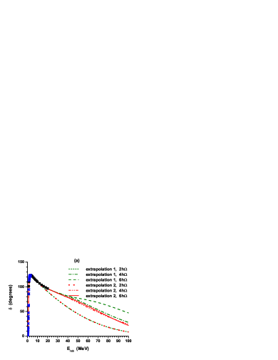
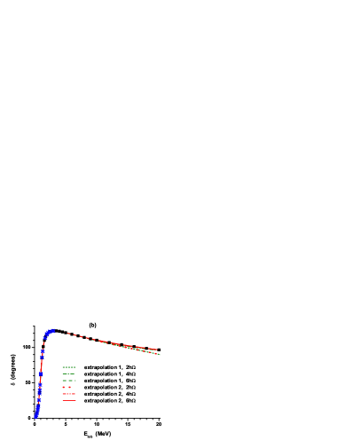
Figure 1: (Color online) Experimental $\frac{3}{2}^{-}$ $n\alpha$ phase shifts from Refs. ArndtDLRop (stars) and NPA287 (filled squares) and $J$-matrix parameterizations with two arbitrary extrapolations of phase shifts for $E_{lab}>20$ MeV obtained with $\hbar\Omega=20$ MeV in $2\hbar\Omega$, $4\hbar\Omega$ and $6\hbar\Omega$ model spaces. Both panels present the same results in different energy scales.

We address the problem of data insufficiency by an extrapolation of the data outside the energy interval of known phase shifts. The $J$-matrix parameterizations presented in Fig. 1 were obtained with $\hbar\Omega=20$ MeV in various model spaces. In each case two different extrapolations were used for the phase shifts at energies $E_{lab}>20$ MeV, however the experimental phase shifts below $E_{lab}=20$ MeV are equivalently well described if $N_{\max}$ is large enough. The deviation of the parameterization from the experiment is seen at energies $E_{lab}>10$ MeV only in the case of the $2\hbar\Omega$ model space, the smallest among all model spaces presented in Fig. 1, and even in this case the deviation is small enough. This is not surprising since the phase shifts given by Eqs. (7) and (13) in the low-energy interval are governed mostly by the $E_{\lambda}$ values from the same interval and by the respective eigenvector components $\langle{\cal N}|\lambda\rangle$. These $E_{\lambda}$ and $\langle{\cal N}|\lambda\rangle$ values are determined by Eqs. (21) and (22) locally, i. e. they are independent from the phase shift extrapolation. Note that in the case of the $2\hbar\Omega$ model space, both $E_{\lambda}$ values lie in the energy interval of known phases, hence the parameterization in this model space is completely independent from the extrapolation and the two parameterizations obtained in this model space coincide.

The resonance energy $E_{res}$ and width $\Gamma$ calculated by locating the $S$-matrix pole by solving Eq. (20), are seen from Table 1 to be very stable and insensitive to the extrapolation of the phase shifts.

Table 1: The energy $E_{res}$ and width $\Gamma$ (both in MeV) of the $\frac{3}{2}^{-}$ resonance in the $n\alpha$ scattering obtained with $\hbar\Omega=20$ MeV in various model spaces $N_{\max}\hbar\Omega$ with two different extrapolations of the phase shifts.

	Extrapolation 1		Extrapolation 2
$N_{\max}$	$E_{res}$	$\Gamma$	$E_{res}$	$\Gamma$
6	0.7713	0.6437	0.7718	0.6435
8	0.7719	0.6451	0.7715	0.6454
10	0.7707	0.6417	0.7708	0.6416

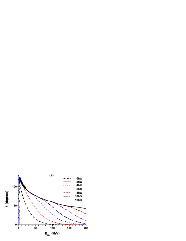
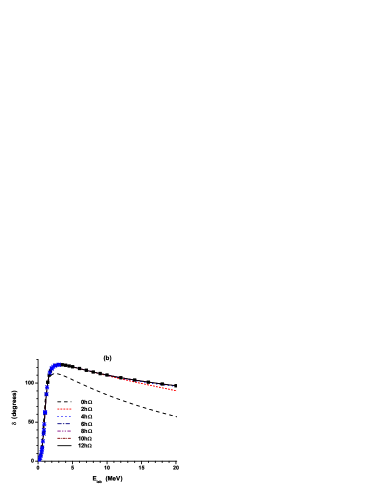
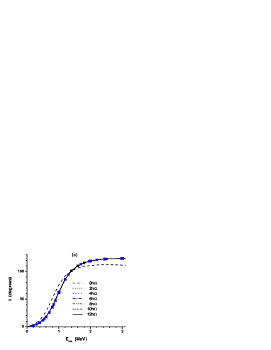
Figure 2: (Color online) The $J$-matrix parameterization of the $\frac{3}{2}^{-}$ $n\alpha$ phase shifts obtained with $\hbar\Omega=20$ MeV in various model spaces. Different panels present the same results in different energy scales. Experimental phase shifts: stars — Ref. ArndtDLRop , filled squares — Ref. NPA287 .

The same insensitivity of the phase description in the desired energy interval to the phase shift extension outside this interval, is also inherent for other $n\alpha$ partial waves. Hence, we shell not waste space by discussing this issue in the respective subsections below. We should probably just note here that the need for data extrapolation arose only due to our desire to compare the $J$-matrix results with the shell model ones; it is this desire that pushes us to use large enough model spaces and $\hbar\Omega$ values. If one is interested only in getting a high quality $J$-matrix parameterization of the phase shifts and in extracting resonance parameters, smaller model spaces and/or smaller $\hbar\Omega$ values can be used without a loss of accuracy and without a need to have phase shifts outside the experimentally known energy interval.

A resulting practical approach is to extrapolate the phase shifts in any reasonable way outside the energy interval where they are known in order to obtain the $J$-matrix parameterization of the phase shifts within this interval of known phases and to derive resonance parameters in the same energy interval. Using such extrapolation, we study a dependence of the $J$-matrix phase shift parameterization on the size of the model space. As is seen from Fig. 2, larger model spaces make it possible to describe the extrapolated phase shifts up to larger energies. The experimental data are perfectly reproduced in $4\hbar\Omega$ and larger model spaces. We fail to reproduce the experiment for $E_{lab}>12$ MeV in the $2\hbar\Omega$ model space. Note however that deviations from the experiment are not very large and we obtain a very good description of the phase shifts at laboratory energies below 12 MeV including the resonance region. The smallest possible $0\hbar\Omega$ model space fails to provide a reasonable description of the phase shifts at all energies.

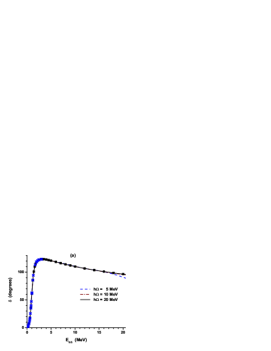
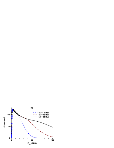
Figure 3: (Color online) The $J$-matrix parameterization of the $\frac{3}{2}^{-}$ $n\alpha$ phase shifts obtained in the $6\hbar\Omega$ model space with different values of oscillator spacing $\hbar\Omega$. See Fig. 2 for details.

As mentioned above, the description of the phase shifts can be extended to larger energies not only by using larger model spaces but also by using larger $\hbar\Omega$ values. This is illustrated by Fig. 3. Even with $\hbar\Omega=5$ MeV we manage to describe the phase shifts in the $6\hbar\Omega$ model space up to approximately $E_{lab}=17$ MeV. The description of all experimentally known phase shifts is perfect in this model space with $\hbar\Omega=10$ MeV and larger.

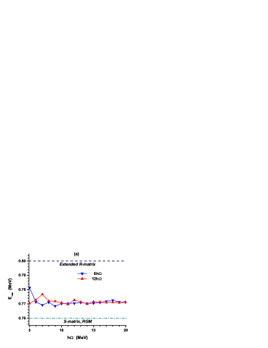
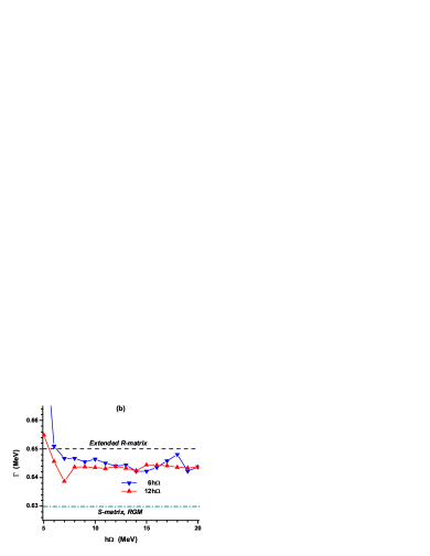
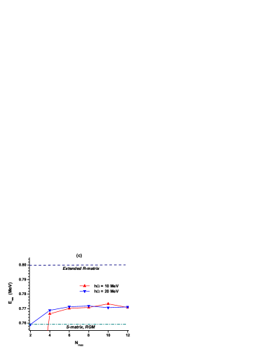
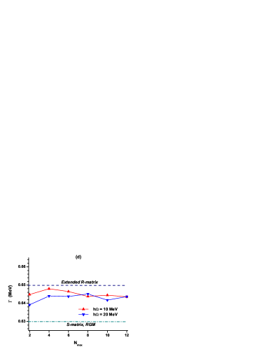
Figure 4: (Color online) The $n\alpha$ $\frac{3}{2}^{-}$ resonance energy in the center-of-mass frame (left) and width (right) obtained by calculating the position of the $S$-matrix pole by means of the $J$-matrix parameterizations with different $\hbar\Omega$ values (upper panels) and in different model spaces (lower panels). Horizontal lines present the results of Ref. Rmatr : the analysis of the resonance parameters in the extended $R$-matrix approach (dashed) and calculations of the $S$-matrix pole position in the Resonating Group Method (dash-dotted).

The results of calculations of the $S$-matrix pole position are presented in Fig. 4. The calculated resonance energy $E_{res}$ and width $\Gamma$ are seen to be very stable in a wide range of $\hbar\Omega$ values and model spaces (note a very detailed energy scale in Fig. 4). Our results are in a very good correspondence with the results of a detailed study of Ref. Rmatr . The authors of this paper performed Resonating Group Method calculations of $N\alpha$ scattering with phenomenological Minnesota $NN$ interaction fitted to reproduce with high precision the $n\alpha$ and $p\alpha$ phase shifts and calculated the position of the $S$-matrix pole. The extended multichannel $R$-matrix analysis of ⁵He and ⁵Li including two-body channels $N+\alpha$ and $d+t$ or $d+\rm^{3}He$ along with pseudo-two-body configurations to represent the breakup channels $n+p+t$ or $n+p+\rm^{3}He$, was also performed in Ref. Rmatr using data of various authors on the differential elastic scattering cross sections, polarization, analyzing-power and polarization-transfer measurements together with neutron total cross sections. Our very simple $J$-matrix analysis utilizing only the elastic scattering phase shifts, is competitive in quality of resonance parameter description with these extended studies of Ref. Rmatr .

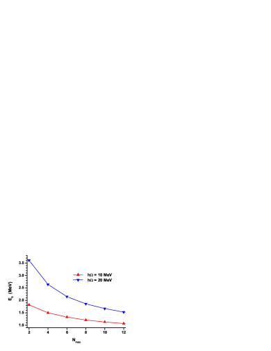
Figure 5: (Color online) The lowest state $E_{\lambda=0}$ obtained in the $J$-matrix parameterization of the $\frac{3}{2}^{-}$ $n\alpha$ phase shifts with different $\hbar\Omega$ values in various model spaces.

We note that while the phase shifts and resonance parameters are very stable, the energies $E_{\lambda}$ entering Eq. (13) vary essentially with $\hbar\Omega$ and model space. In particular, this is true for the lowest of these energies $E_{\lambda=0}$ shown in Fig. 5 (note a very large difference in energy scales in Figs. 4 and 5). This energy being obtained in shell model studies, would be associated traditionally with the resonance energy $E_{res}$. Such a conventional association is clearly incorrect: this lowest eigenstate $E_{\lambda=0}$ differs significantly in energy from $E_{res}$ while the phase shifts and resonance energy and width are well reproduced; just this energy $E_{\lambda=0}$, very different from $E_{res}$, is needed to have a perfect description of scattering data and resonance parameters including $E_{res}$ itself. The $E_{\lambda=0}$ dependencies of the type shown in Fig. 5 are inherent in other partial waves and in the case of $p\alpha$ scattering. We study the $E_{\lambda=0}$ dependencies on $\hbar\Omega$ and model space in more detail below in Section V where we compare them with the results of No-core Shell Model calculations.

III.2 $\frac{1}{2}^{-}$ phase shifts

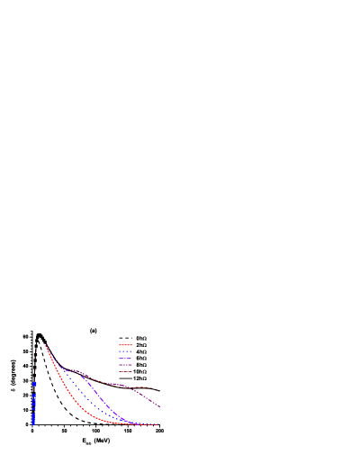
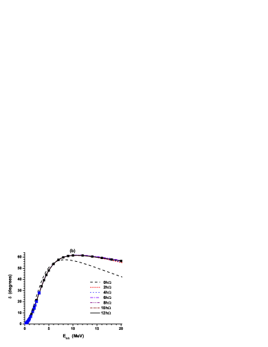
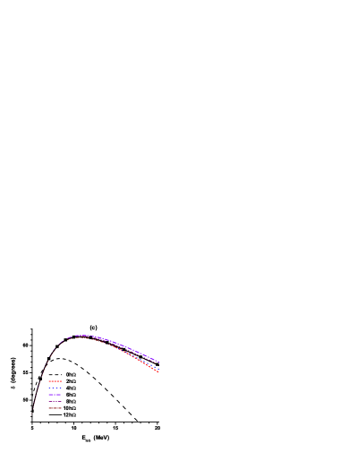
Figure 6: (Color online) The $J$-matrix parameterization of the $\frac{1}{2}^{-}$ $n\alpha$ phase shifts obtained with $\hbar\Omega=20$ MeV in various model spaces. See Fig. 2 for details.

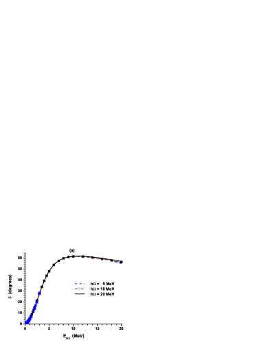
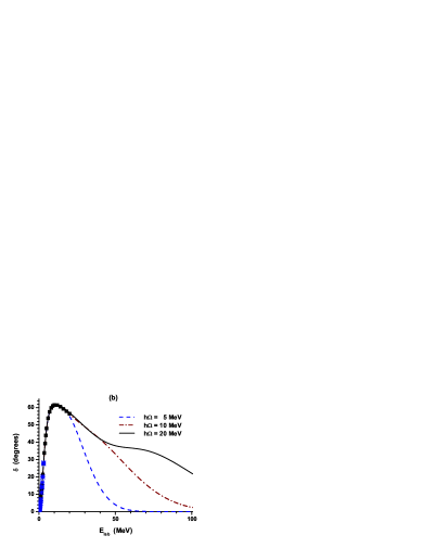
Figure 7: (Color online) The $J$-matrix parameterization of the $\frac{1}{2}^{-}$ $n\alpha$ phase shifts obtained in the $6\hbar\Omega$ model space with different values of oscillator spacing $\hbar\Omega$. See Fig. 3 for details.

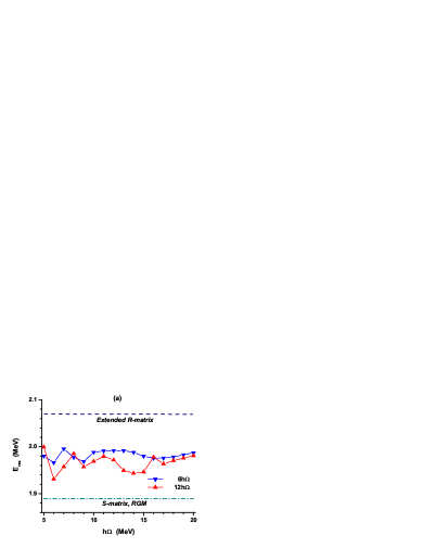
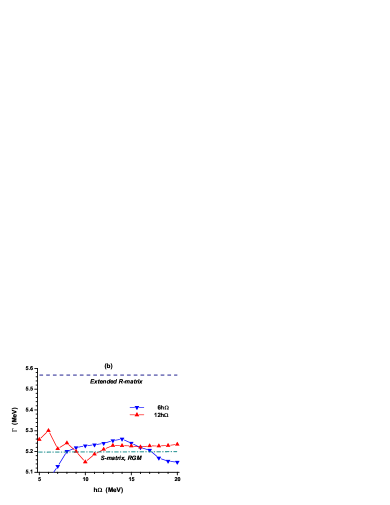
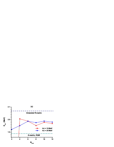
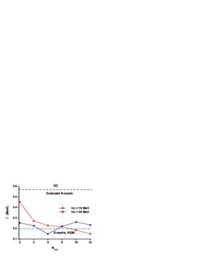
Figure 8: (Color online) The $n\alpha$ $\frac{1}{2}^{-}$ resonance energy in the center-of-mass frame (left) and width (right) obtained by calculating the position of the $S$-matrix pole by means of the $J$-matrix parameterizations with different $\hbar\Omega$ values (upper panels) and in different model spaces (lower panels). See Fig. 4 for details.

We present in Figs. 6 and 7 respectively the $J$-matrix parameterizations of $n\alpha$ $\frac{1}{2}^{-}$ phase shifts obtained with the same $\hbar\Omega$ in different model spaces and with different $\hbar\Omega$ values in the same model space. The description of the $\frac{1}{2}^{-}$ phase shifts with different $\hbar\Omega$ values and in different model spaces follows the same patterns as in the case of the $\frac{3}{2}^{-}$ phase shifts. The only difference is that a high-quality description of the phase shifts at energies $E_{lab}>10$ MeV is attained in larger model spaces. However, in the $8\hbar\Omega$ and larger model spaces the description of all known phase shifts is perfect.

Figure 8 presents the results of our calculations of the $\frac{1}{2}^{-}$ resonance energy and width. The variations of $E_{res}$ and $\Gamma$ with increasing $\hbar\Omega$ or model space are larger than in the case of the $\frac{3}{2}^{-}$ resonance; note however that the energy of the $\frac{1}{2}^{-}$ resonance and its width are also much larger. At any rate, the variations of resonance parameters are not large and our results for $E_{res}$ and $\Gamma$ are stable enough with respect to the choice of $\hbar\Omega$ value and model space. The energy and width of the $\frac{1}{2}^{-}$ resonance also compare well with the results of Ref. Rmatr .

III.3 $\frac{1}{2}^{+}$ phase shifts

In describing the $\frac{1}{2}^{+}$ phase shifts, one should have in mind that the lowest $s$ states are occupied in the $\alpha$-particle and due to the Pauli principle these states should be inaccessible to the scattered nucleon. There are two conventional approaches to the problem of the Pauli forbidden $s$ state in the $n+\alpha$ system. The first approach is to add a phenomenological repulsive term to the $s$ wave component of the $n\alpha$ potential (see, e. g., Rep-na ). This phenomenological repulsion excludes the Pauli forbidden state in the $n+\alpha$ system and is supposed to simulate the Pauli principle effects in more complicated cluster systems. Another approach is to use deep attractive $n\alpha$ potentials that support the Pauli forbidden $s$ state in the $n+\alpha$ system (see Forb-na ; Kuku ; Forb-na2 ). In the cluster model studies, the Pauli forbidden state is excluded by projecting it out Kuku ; Forb-na2 ; LurAnn .

In our $J$-matrix inverse scattering approach, we can simulate both the potentials with repulsive core and with a forbidden state. In the first case, when the system does not have a bound state, we go on with the same procedure as in the above cases of $\frac{3}{2}^{-}$ and $\frac{1}{2}^{-}$ partial waves; the energy dependence of the input $\frac{1}{2}^{+}$ phase shifts is responsible for generating proper details of the $n\alpha$ interaction potential matrix. In the other case, the simplest way to simulate the presence of the forbidden state in the system is to suppose that this state is described by a pure $0s_{1/2}$ oscillator wave function. The energy of the forbidden state is equal in this case to the Hamiltonian matrix element $H_{00}^{l=0}$ which is of no interest for us in this study, all the matrix elements $H_{0n}^{l=0}$ and $H_{n0}^{l=0}$ should be set equal to zero to guarantee the orthogonality of the forbidden state to scattering states which have the wave functions given by the expansion (2) where the $0s_{1/2}$ oscillator state is missing, i. e. $a_{n=0,\,l=0}(E)=0$ for all energies $E>0$. Within this model, the forbidden state IS does not contribute to the function ${\cal G}_{\cal NN}(E)$ [see Eq. (13)] since the component $\langle{\cal N}|\lambda=0\rangle=0$. In the inverse scattering approach, we use the first $\cal N$ solutions of Eq. (21) disregarding the highest in energy solution $E_{{\cal N}+1}$ while constructing the function ${\cal G}_{\cal NN}(E)$.

In Fig. 9 we present the $J$-matrix parameterization of the $\frac{1}{2}^{+}$ phase shifts in elastic $n\alpha$ scattering in the $7\hbar\Omega$ model space with different values of the oscillator spacing $\hbar\Omega$. As usual, larger $\hbar\Omega$ value makes it possible to describe the phase shifts in a larger energy interval. A new and interesting issue is the difference in behavior of the phase shifts in the models with and without a forbidden state. A more realistic model with forbidden state provides a proper dependence of the phase shifts: starting with $180^{\circ}$ at zero energy, they tend to zero at large energies. The forbidden state makes the same contribution to the Levinson theorem as any other bound state providing the $180^{\circ}$ difference between the phase shifts at zero and infinite energies. The model without a forbidden state generates the phase shifts returning at large energies back to their zero energy value. In what follows, we use the potential model with a forbidden state. Note however that in the energy interval of known phase shifts, the parameterizations of both models are indistinguishable. The $E_{\lambda}$ values provided by both models in this energy interval, are the same.

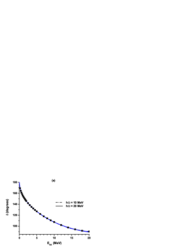
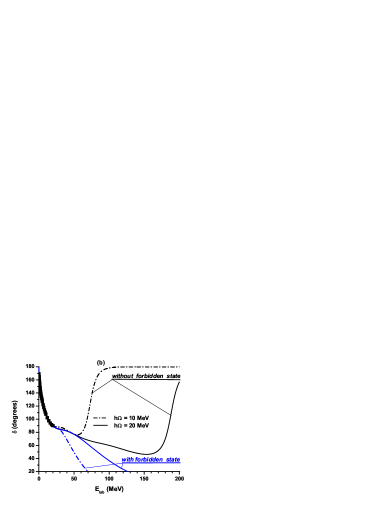
Figure 9: (Color online) The $J$-matrix parameterization of the $\frac{1}{2}^{+}$ $n\alpha$ phase shifts obtained in the $7\hbar\Omega$ model space with different values of oscillator spacing $\hbar\Omega$. See Fig. 3 for details.

The $\frac{1}{2}^{+}$ phase shifts parameterizations in different model spaces with $\hbar\Omega=20$ MeV perfectly describe the data (Fig. 10). At larger energies, they follow general trends: smaller model spaces result in a faster fall off of the phase shifts to zero value.

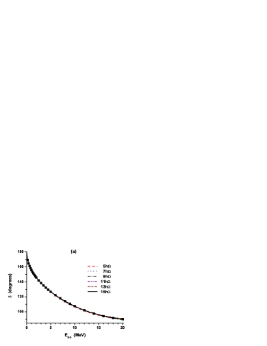
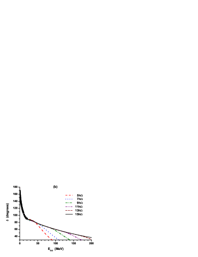
Figure 10: (Color online) The $J$-matrix parameterization of the $\frac{1}{2}^{+}$ $n\alpha$ phase shifts obtained in the model with forbidden state with $\hbar\Omega=20$ MeV in various model spaces. See Fig. 3 for details.

IV Analysis of $p\alpha$ scattering phase shifts

IV.1 $\frac{3}{2}^{-}$ phase shifts

The $J$-matrix approach to $p\alpha$ scattering involves an additional parameter $b$, the channel radius used to define the auxiliary potential $V^{Sh}$ by truncating the Coulomb interaction at $r=b$ [see Eq. (32)]. We start our discussion of the $J$-matrix inverse scattering description of $p\alpha$ scattering from the analysis of the $b$-dependence of the $\frac{3}{2}^{-}$ $p\alpha$ phase shift parameterization.

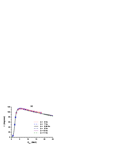
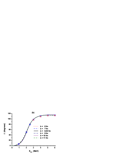
Figure 11: (Color online) The $J$-matrix parameterization of the $\frac{3}{2}^{-}$ $p\alpha$ phase shifts obtained with $\hbar\Omega=20$ MeV in the $10\hbar\Omega$ model space with various $b$ values. Two panels present the same results in different scales. Experimental phase shifts: open squares — Ref. Arndt , open circles — Ref. NPA163 , crosses — Ref. Dodder .

We present in Fig. 11 the $p\alpha$ $\frac{3}{2}^{-}$ phase shift parameterizations obtained with different channel radii $b$ in the $10\hbar\Omega$ model space with $\hbar\Omega=20$ MeV. The experimental data are seen to be perfectly described in the interval of $b$ values $\rm 6~{}fm\leq b\leq 10~{}fm$. However we did not find a way to reproduce accurately the phase shifts with $b\geq 11$ fm, in particular at energies between 10 and 20 MeV. This is not surprising since the classical turning point of the highest oscillator function $R_{{\cal N}l}(r)$ involved in the construction of the truncated Hamiltonian $H^{l}_{nn^{\prime}}$ $(n,n^{\prime}\leq{\cal N})$, $r^{cl}_{\cal N}=8.06$ fm in this case. The $\frac{3}{2}^{-}$ resonance energy and width dependences on $b$ obtained from these parameterizations, are shown in Fig. 12. The resonance parameters are seen to be stable enough with $b$ varying between 6 and 10 fm. The $b$ dependence of the energy $E_{\lambda=0}$ of the lowest state obtained in the $J$-matrix parameterization, has a plateau between 7 and 10 fm (see Fig. 13).

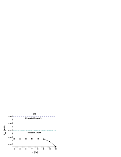
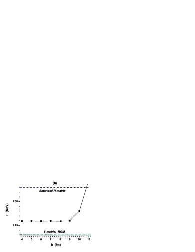
Figure 12: (Color online) Dependence of the $\frac{3}{2}^{-}$ $p\alpha$ resonance energy in the center-of-mass frame (upper panel) and width (lower panel) on the channel radius $b$ in the $10\hbar\Omega$ model space calculations with $\hbar\omega=20$ MeV. See Fig. 4 for details.

Figure 13: The $b$ dependence of the lowest state $E_{\lambda=0}$ in the $10\hbar\Omega$ model space $J$-matrix parameterizations with $\hbar\omega=20$ MeV.

The bottom line of these studies is that the results are nearly $b$-independent for $b$ values in some vicinity of the classical turning point $r^{cl}_{\cal N}$. This conclusion remains valid for other partial waves of the $p\alpha$ scattering and we are not discussing $b$-dependences in the following subsections. The remainder of the calculations presented here are performed with $b=r^{cl}_{\cal N}$.

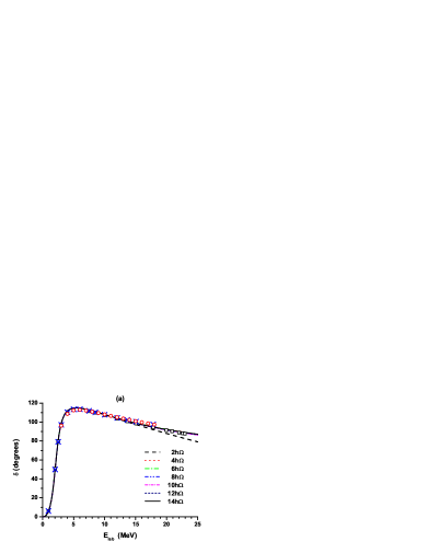
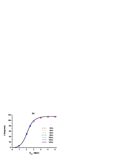
Figure 14: (Color online) The $J$-matrix parameterization of the $p\alpha$ $\frac{3}{2}^{-}$ phase shifts obtained with $\hbar\Omega=20$ MeV in various model spaces. See Fig. 11 for details.

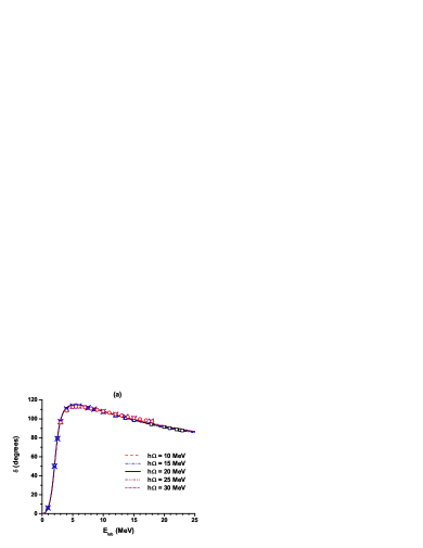
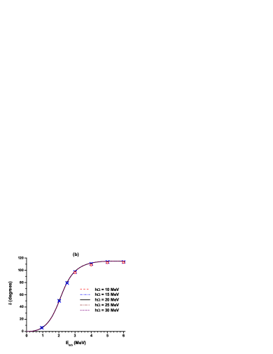
Figure 15: (Color online) The $J$-matrix parameterization of the $p\alpha$ $\frac{3}{2}^{-}$ phase shifts obtained in the $10\hbar\Omega$ model space with various $\hbar\Omega$ values. See Fig. 11 for details.

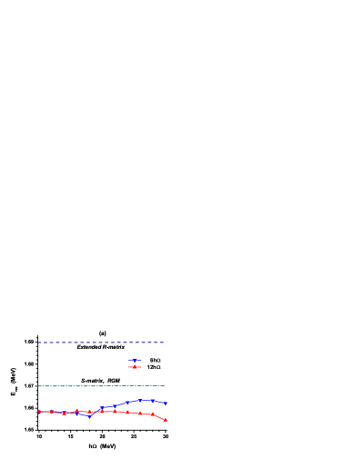
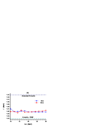
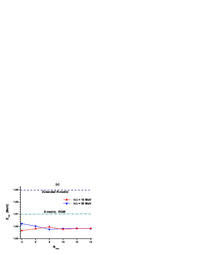
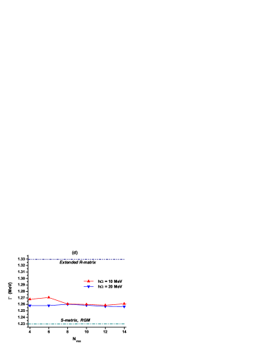
Figure 16: (Color online) The $p\alpha$ $\frac{3}{2}^{-}$ resonance energy in the center-of-mass frame (left) and width (right) obtained by calculating the position of the $S$-matrix pole by means of the $J$-matrix parameterizations with different $\hbar\Omega$ values (upper panels) and in different model spaces (lower panels). See Fig. 4 for details.

We present in Fig. 14 the $J$-matrix parameterization of the $\frac{3}{2}^{-}$ $p\alpha$ phase shifts obtained in various model spaces with $\hbar\Omega=20$ MeV. The data are well-described in $4\hbar\Omega$ and higher model spaces. Some deviation from experiment is seen only for the $2\hbar\Omega$ model space starting from laboratory energies about 20 MeV. However, the resonance region is perfectly described even in this very small $2\hbar\Omega$ model space as is seen from the lower panel of Fig. 14 where the enlarged energy scale is used. The $J$-matrix parameterization is also insensitive to the variation of the $\hbar\Omega$ value in the whole interval of known phase shifts including the resonance region (see Fig. 15). Therefore it is not surprising that we obtain a very stable description of the resonance energy and width (see Fig. 16), one that is independent of the model space and $\hbar\Omega$ value.

Our results for the $\frac{3}{2}^{-}$ resonance parameters are very close to the ones obtained in the analysis of Ref. Rmatr .

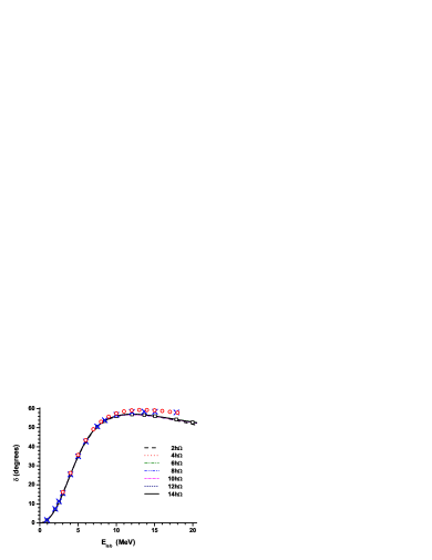
Figure 17: (Color online) The $J$-matrix parameterization of the $p\alpha$ $\frac{1}{2}^{-}$ phase shifts obtained with $\hbar\Omega=20$ MeV in various model spaces. See Fig. 11 for details.

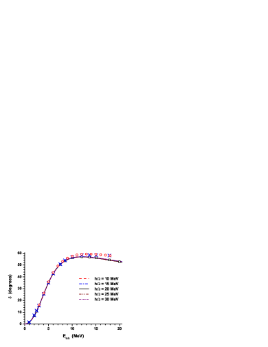
Figure 18: (Color online) The $J$-matrix parameterization of the $p\alpha$ $\frac{1}{2}^{-}$ phase shifts obtained in the $10\hbar\Omega$ model space with various $\hbar\Omega$ values. See Fig. 11 for details.

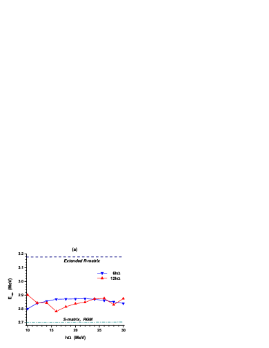
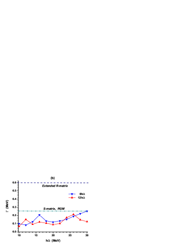
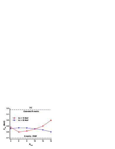
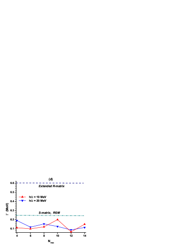
Figure 19: (Color online) The $p\alpha$ $\frac{1}{2}^{-}$ resonance energy in the center-of-mass frame (left) and width (right) obtained by calculating the position of the $S$-matrix pole by means of the $J$-matrix parameterizations with different $\hbar\Omega$ values (upper panels) and in different model spaces (lower panels). See Fig. 4 for details.

IV.2 $\frac{1}{2}^{-}$ phase shifts

We obtain a high-quality $J$-matrix parameterization of the $p\alpha$ $\frac{1}{2}^{-}$ phase shifts, very stable with variations of the model space or oscillator spacing $\hbar\Omega$. A small deviation from the experiment at large energies is seen in Fig. 17 in the $2\hbar\Omega$ model space only. The parameterizations obtained in the $10\hbar\Omega$ model space with $\hbar\Omega$ values ranging from 10 to 30 MeV, are indistinguishable in Fig. 18. The resonance region is perfectly described. Our results for the resonance energy and width correspond well to the analysis of Ref. Rmatr . The resonance parameters are stable with respect to variations of the model space and $\hbar\Omega$ (see Fig. 19). Of course, the variations of $E_{res}$ and $\Gamma$ in Fig. 19 are much larger than in the case of the $\frac{3}{2}^{-}$ resonance, but the $\frac{1}{2}^{-}$ resonance energy and width are also much larger than the energy and width of the $\frac{3}{2}^{-}$ resonance.

IV.3 $\frac{1}{2}^{+}$ phase shifts

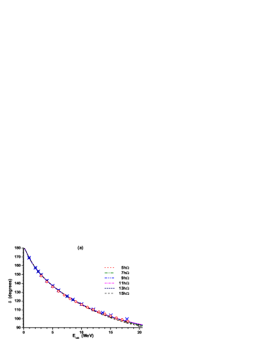
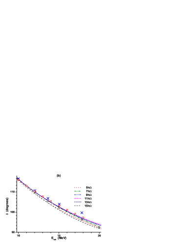
Figure 20: (Color online) The $J$-matrix parameterization of the $p\alpha$ $\frac{1}{2}^{+}$ phase shifts obtained in the model with forbidden state with $\hbar\Omega=20$ MeV in various model spaces. See Fig. 11 for details.

In the case of $s$ wave of $p\alpha$ scattering, we can also use interaction models with and without a forbidden state. The main features of the $J$-matrix parameterizations within these models in the case of the $p\alpha$ scattering are the same as in the case of $n\alpha$ scattering; in particular, the phase shift description in the low-energy region covering the whole region of known phase shifts, is identical within these interaction models. In what follows, we present only the results obtained in the model with forbidden state which we suppose to be more realistic.

The $J$-matrix parameterizations of the $p\alpha$ $\frac{1}{2}^{+}$ phase shifts obtained in various model spaces with $\hbar\Omega=20$ MeV, are presented in Fig. 20 in two scales. The low-energy phase shifts up to approximately $E_{lab}=10$ MeV are perfectly reproduced in all model spaces. Starting from $E_{lab}=10$ MeV, there are some deviations from the experiment that are well seen in the right panel of Fig. 20 where a larger scale is used. Surprisingly, the deviations from experimental phase shifts are larger in larger model spaces. The deviations are not large but not negligible.

The $J$-matrix parameterizations obtained with various $\hbar\Omega$ values in the $11\hbar\Omega$ model space, are shown in Fig. 21. The theoretical curves are nearly indistinguishable below $E_{lab}=10$ MeV reproducing well the experimental data. Some difference between parameterizations is seen in the high-energy part of the interval of known phase shifts. All $J$-matrix parameterizations presented in Fig. 21 reasonably describe the phenomenological data in the whole energy interval of known phase shifts. The worst description of the phase shifts in the $11\hbar\Omega$ model space is obtained with $\hbar\Omega=15$ MeV.

V $J$-matrix and shell model eigenstates

Up to now, we were discussing the $J$-matrix inverse scattering description of scattering observables in the $n+\alpha$ and $p+\alpha$ nuclear systems. It is very interesting to investigate whether these observables correlate with the shell model predictions for ⁵He and ⁵Li nuclei. It should be done, as we have shown above, by comparing the eigenenergies $E_{\lambda}$ obtained in the $J$-matrix inverse scattering approach with the energies of the states obtained in the shell model.

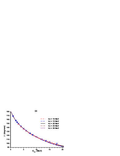
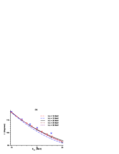
Figure 21: (Color online) The $J$-matrix parameterization of the $p\alpha$ $\frac{1}{2}^{+}$ phase shifts obtained in the model with forbidden state in the $11\hbar\Omega$ model space with various $\hbar\Omega$ values. See Fig. 11 for details.

We calculate the lowest ⁵He and ⁵Li states of a given spin and parity in the No-core Shell Model approach Vary using the code MFDn Vary92_MFDn and the JISP16 nucleon-nucleon interaction JISP16 ; JWEB . We do not make use of effective interactions calculated within Lee–Suzuki or any other approach. That is, all results presented here are obtained with the ‘bare’ JISP16 $NN$ interaction which is known JISP16 ; JISPYaF ; extrap08 to provide a reasonable convergence as basis space size increases. One may note that the No-Core Shell Model with a bare interaction and with a truncated configuration basis may also be referred to as a “configuration interaction” or “CI” type calculation Roth .

In all cases, the calculations of the ⁴He ground state energy is performed with the same $\hbar\Omega$ value and in the same $N_{\max}\hbar\Omega$ model space. These ⁴He ground state energies are used to calculate the reaction threshold while comparing the $J$-matrix $E_{\lambda}$ values (defined with regard to the reaction threshold) with the shell model results. Therefore our reaction threshold is model space and $\hbar\Omega$-dependent, however these dependencies are strongly suppressed in large enough model spaces. This definition of the reaction threshold is, of course, somewhat arbitrary. We use it supposing that our definition provides a consistent way to generate energies relative to the ⁴He ground state energy within the No-core Shell Model approach employing a finite basis.

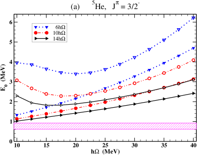
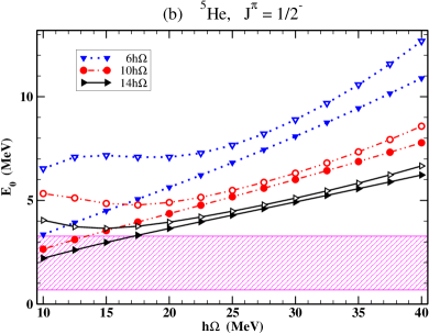
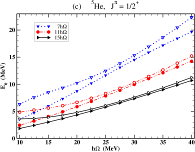
Figure 22: (Color online) $E_{\lambda=0}$ values for $n\alpha$ scattering obtained in the $J$-matrix inverse scattering approach in the center-of-mass frame (filled symbols) and respective lowest eigenstates of the ⁵He nucleus obtained in the No-core Shell Model (respective empty symbols). The resonance energies together with their widths are shown by shaded areas.

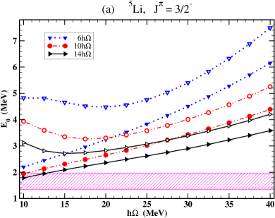
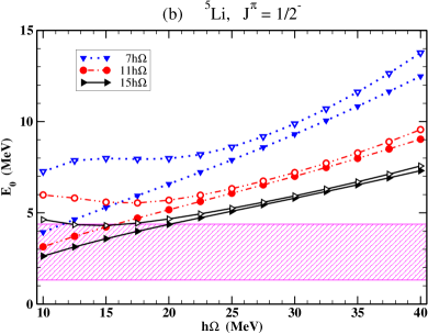
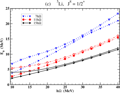
Figure 23: (Color online) $E_{\lambda=0}$ values for $p\alpha$ scattering obtained in the $J$-matrix inverse scattering approach in the center-of-mass frame and respective lowest eigenstates of the ⁵Li nucleus obtained in the No-core Shell Model. See Fig. 22 for details.

The No-core Shell Model results for the lowest ⁵He and ⁵Li $\frac{3}{2}^{-}$, $\frac{1}{2}^{-}$ and $\frac{1}{2}^{+}$ states are compared with the respective $J$-matrix $E_{\lambda=0}$ values in Figs. 22 and 23. For each spin and parity, the $J$-matrix $E_{\lambda=0}$ values obtained with the same $\hbar\Omega$ value, are seen to decrease with increasing model space (see also Fig. 5); the same model space dependence is well-known to be inherent for the shell model eigenstates. However the $\hbar\Omega$ dependences of the $J$-matrix $E_{\lambda=0}$ and shell model eigenstates, are very different: the shell model eigenstates are known to have a minimum at some $\hbar\Omega$ value while the inverse scattering $E_{\lambda=0}$ are seen from Figs. 22 and 23 to increase nearly linearly with $\hbar\Omega$; the slope of the $\hbar\Omega$ dependence of $E_{\lambda=0}$ is larger for wider resonances. As a result, the shell model predictions differ from the results of the inverse scattering analysis for small enough $\hbar\Omega$ values. However, a remarkable correspondence between the shell model and inverse scattering results is seen at large enough $\hbar\Omega$ values starting from approximately $\hbar\Omega=20$ MeV. The agreement between the shell model and $J$-matrix inverse scattering analysis is improved with increasing model space; it is probable that this is partly due to the improvement in larger model spaces of the calculated threshold energy in our approach. The shell model description of the lowest $\frac{1}{2}^{-}$ and $\frac{1}{2}^{+}$ states is somewhat better than the lowest $\frac{3}{2}^{-}$ state description in both ⁵He and ⁵Li nuclear systems. The lowest $\frac{3}{2}^{-}$ state description is however not so bad (note a more detailed energy scale for the $\frac{3}{2}^{-}$ state in Figs. 22 and 23): the difference between the shell model predictions and the $J$-matrix analysis results is about 0.5 MeV in large enough model spaces and for large enough $\hbar\Omega$ values. An excellent description of the $\frac{1}{2}^{-}$ states in ⁵He and ⁵Li combined with some deficiency in description of the $\frac{3}{2}^{-}$ states in the same nuclei, is probably a signal of a somewhat underestimated strength of the spin-orbit interaction generated by the JISP16 $NN$ interaction in the $p$ shell.

We suppose that the results presented here illustrate well the power of the proposed $J$-matrix analysis, a new method that makes it possible to verify a consistency of shell model results with experimental phase shifts. To the best of our knowledge, this is the only method which can relate the shell model results to the scattering data in the case of non-resonant scattering like the $\frac{1}{2}^{+}$ $n\alpha$ and $p\alpha$ scattering. In the case of negative parity resonances in ⁵He and ⁵Li discussed here, the $J$-matrix analysis generally suggests that the shell model should generate the respective states above the resonance energies supplemented by their widths. Note that the $J$-matrix $E_{\lambda=0}$ only in some cases lie inside shaded areas showing the resonance energies together with their widths in Figs. 22 and 23, and in all these cases, the intersection of the $E_{\lambda=0}$ with the resonance is seen only at small enough $\hbar\Omega$ values where the shell model predictions fail to follow the $J$-matrix analysis results. This is a clear indication that one should be very accurate in relating the shell model results to the resonance energies, at least in the case of wide enough resonances.

VI Conclusions

We suggest a method of $J$-matrix inverse scattering analysis of elastic scattering phase shifts and test this method in applications to $n\alpha$ and $p\alpha$ elastic scattering. We demonstrate that the method is able to reproduce $\frac{3}{2}^{-}$, $\frac{1}{2}^{-}$ and $\frac{1}{2}^{+}$ $n\alpha$ and $p\alpha$ elastic scattering phase shifts with high accuracy in a wide range of the parameters of the method like the oscillator spacing $\hbar\Omega$, model space and the channel radius $b$ in the case of $p\alpha$ scattering. The method is very simple in applications, it involves only a numerical solution of a simple transcendental equation (21).

When the $J$-matrix phase shift parameterization is obtained, the resonance parameters, resonance energy and width, can be obtained by locating the $S$-matrix pole by solving numerically another simple transcendental equation (20). The resonance energies and widths are shown to be stable when $\hbar\Omega$ or other $J$-matrix parameters are varied. Our results for $\frac{3}{2}^{-}$ and $\frac{1}{2}^{-}$ resonant states in ⁵He and ⁵Li are compared in Table 2 with the results of other authors. Our results are in line with the results of other studies; in general, the better agreement is seen with Ref. Rmatr , the most recent among all publications presented in the Table. Csótó and Hale performed two different analyses in Ref. Rmatr : (i) RGM search for the $S$-matrix poles based on a complicated enough calculations within the Resonating Group Model with effective Minnesota $NN$ interaction fitted to the nucleon-$\alpha$ phase shifts, and (ii) Extended $R$-matrix analysis of ⁵He and ⁵Li including not only $N+\alpha$ channel but also $d+t$ or $d+\rm^{3}He$ channels along with pseudo-two-body configurations to represent the breakup channels $n+p+t$ or $n+p+\rm^{3}He$ and using a wide range of data on various reactions. We note that our very simple $J$-matrix approach uses only a very limited set of data as an input, $n\alpha$ or $p\alpha$ phase shifts. We suppose that the proposed approach can be useful in analysis of elastic scattering in other nuclear systems and serve as an alternative to the conventional $R$-matrix analysis.

Table 2: Parameters of the low-energy ⁵He and ⁵Li resonances in the center-of-mass frame. All numbers are in MeV. The uncertainty of our results was evaluated as the maximal deviation in calculations in model spaces ranging from $6\hbar\Omega$ to $14\hbar\Omega$ and with $\hbar\Omega$ values ranging from 10 to 30 MeV.

	5He				5Li
Method	$E_{res}(3/2^{-})$	$\Gamma(3/2^{-})$	$E_{res}(1/2^{-})$	$\Gamma(1/2^{-})$	$E_{res}(3/2^{-})$	$\Gamma(3/2^{-})$	$E_{res}(1/2^{-})$	$\Gamma(1/2^{-})$
Compilation AjSe	$0.89\pm 0.05$	$0.60\pm 0.02$	$4.89\pm 1$	$4\pm 1$	$1.96.\pm 0.05$	$\approx 1.5$	7$-$12	$5\pm 2$
$R$-matrix, stripping AusJPh	$0.838\pm 0.018$	$0.645\pm 0.046$	$2.778\pm 0.46$	$3.6\pm 1.2$	$1.76\pm 0.06$	$1.18\pm 0.13$	$3.63\pm 0.56$	$4.1\pm 2.5$
$R$-matrix, pickup AusJPh	$0.869\pm 0.003$	$0.723\pm 0.019$	$3.449\pm 0.4$	$5.3\pm 2.3$	$1.86\pm 0.01$	$1.44\pm 0.08$	$4.54\pm 0.5$	$6.1\pm 2.8$
Scattering ampl. ScatAm	0.778	0.639	1.999	4.534	1.637	1.292	2.858	6.082
$S$-matrix, RGM Rmatr	0.76	0.63	1.89	5.20	1.67	1.33	2.70	6.25
Extended $R$-matrix Rmatr	0.80	0.65	2.07	5.57	1.69	1.23	3.18	6.60
$J$-matrix	$0.772\pm 0.005$	$0.644\pm 0.005$	$1.97\pm 0.03$	$5.20\pm 0.05$	$1.658\pm 0.005$	$1.26\pm 0.01$	$2.85\pm 0.05$	$6.15\pm 0.10$

A very interesting and important output of the $J$-matrix inverse scattering analysis of the phase shifts is the set of $E_{\lambda}$ values which are directly related to the eigenenergies obtained in the shell model or any other model utilizing the oscillator basis, for example, the Resonating Group Model. The $J$-matrix parameterizations provide the energies of the states that should be obtained in the shell model or Resonating Group Model to generate the given phase shifts. These energies are shown to be model space and $\hbar\Omega$-dependent and very different from the energies of at least wide enough resonances which are conventionally used to compare with the shell model results. More, the $J$-matrix analysis is shown to provide the shell model energies even in the case of non-resonant scattering such as the $\frac{1}{2}^{+}$ nucleon–$\alpha$ scattering.

Our comparison of the lowest $E_{\lambda=0}$ with the No-core Shell Model results shows that the shell model fails to reproduce the phase shifts if small $\hbar\Omega$ values are employed in the calculations. When $\hbar\Omega$ and/or model space size is increased, the shell model predictions approach $E_{\lambda=0}$ values obtained in the $J$-matrix signaling that the shell model results become more and more consistent with the experimental phase shifts. However some difference between the No-core Shell Model predictions and the $J$-matrix analysis results is seen even in the largest model spaces used in this study. This difference is really not large, its possible sources are the following. (i) There is an ambiguity in the threshold energies used to relate the absolute negative energies obtained in the shell model and positive $E_{\lambda}$ values defined relative to the reaction threshold. (ii) Unfortunately, there is no $NN$ interaction providing correct energies for, at least, light nuclei. The JISP16 $NN$ interaction is good enough and provides reliable predictions for energies of levels in all $s$ and $p$ shell nuclei JISP16 ; JISPYaF ; extrap08 . However, there are small differences between JISP16 level energy predictions and experiment; these differences are of the same order as the differences between the $J$-matrix $E_{\lambda=0}$ values and our No-core Shell Model results. Probably we shall use the $J$-matrix results discussed above while attempting to design a new improved version of the JISP16 interaction by trying to eliminate the discrepancy between the shell model results and the $J$-matrix analysis of nucleon-$\alpha$ scattering.

Of course, the $J$-matrix can be used to relate the shell model energies and data on nucleon scattering by other nuclei. Generally, one can also use other elastic scattering data, for example, nucleus-nucleus elastic scattering phase shifts to get the $E_{\lambda}$ values that should be obtained in the shell model studies of the respective compound nuclear systems: the shell model must generate the states with the same energies in the same model space and with the same $\hbar\Omega$ value to have a chance to generate the experimental phase shifts.

We are thankful to G. M. Hale and P. Maris for valuable discussions and help in our studies. This work was supported in part by the Russian Foundation of Basic Research, by the US DOE Grants DE-FC02-07ER41457 and DE-FG02-87ER40371.

References

- (1) A. M. Lane and R. G. Thomas, Rev. Mod. Phys. 30, 257 (1958).
- (2) H. A. Yamani and L. Fishman, J. Math. Phys. 16, 410 (1975).
- (3) S. A. Zaytsev, Teoret. Mat. Fiz. 115, 263 (1998) [Theor. Math. Phys. 115, 575 (1998)].
- (4) A. M. Shirokov, A. I. Mazur, S. A. Zaytsev, J. P. Vary, and T. A. Weber, Phys. Rev. C 70, 044005 (2004); in The -Matrix Method. Developments and Applications, edited by A. D. Alhaidari, H. A. Yamani, E. J. Heller, and M. S. Abdelmonem (Springer, 2008), 219.
- (5) A. M. Shirokov, J. P. Vary, A. I. Mazur, S. A. Zaytsev, and T. A. Weber, Phys. Lett. B621, 96 (2005); J. Phys. G 31, S1283 (2005).
- (6) A. M. Shirokov, J. P. Vary, A. I. Mazur, and T. A. Weber, Phys. Lett. B644, 33 (2007).
- (7) J. M. Bang, A. I. Mazur, A. M. Shirokov, Yu. F. Smirnov, and S. A. Zaytsev, Ann. Phys. (NY) 280, 299 (2000).
- (8) D. C. Zheng, J. P. Vary, and B. R. Barrett, Phys. Rev. C 50, 2841 (1994); D. C. Zheng, J. P. Vary, B. R. Barrett, W. C. Haxton, and C. L. Song, Phys. Rev. C 52, 2488 (1995).
- (9) A. M. Shirokov, Yu. F. Smirnov, and S. A. Zaytsev, in Modern Problems in Quantum Theory, edited by V. I. Savrin and O. A. Khrustalev, (Moscow State University, Moscow, 1998), 184; Teoret. Mat. Fiz. 117, 227 (1998) [Theor. Math. Phys. 117, 1291 (1998)].
- (10) G. F. Filippov and I. P. Okhrimenko, Yad. Fiz. 32, 932 (1980) [Sov. J. Nucl. Phys. 32, 480 (1980)]; G. F. Filippov, Yad. Fiz. 33, 928 (1981) [Sov. J. Nucl. Phys. 33, 488 (1981)].
- (11) V. I. Kukulin, V. N. Pomerantsev, Kh. D. Razikov, V. T. Voronchev, and G. G. Ryzhikh, Nucl. Phys. A 586, 151 (1995).
- (12) I. P. Okhrimenko, Nucl. Phys. A 424, 121 (1984).
- (13) R. A. Arndt, D. D. Long, and L. D. Roper, Nucl. Phys. A 209, 429 (1973).
- (14) J. E. Bond and F. W. K. Firk, Nucl. Phys. A 287, 317 (1977).
- (15) A. Csótó and G. M. Hale, Phys. Rev. C 55,536 (1997).
- (16) B. V. Danilin, M. V. Zhukov, A. A. Korsheninnikov, and L. V. Chulkov, Yad. Fiz. 53, 71 (1991) [Sov. J. Nucl. Phys. 53, 45 (1991)].
- (17) J. Bang and C. Gignoux, Nucl. Phys. A 313, 119 (1979).
- (18) Yu. A. Lurie and A. M. Shirokov, Izv. Ros. Akad. Nauk, Ser. Fiz. 61, 2121 (1997) [Bull. Rus. Acad. Sci., Phys. Ser. 61, 1665 (1997)].
- (19) Yu. A. Lurie and A. M. Shirokov, Ann. Phys. (NY) 312, 284 (2004); in The -Matrix Method. Developments and Applications, edited by A. D. Alhaidari, H. A. Yamani, E. J. Heller, and M. S. Abdelmonem (Springer, 2008), 183.
- (20) The forbidden state in this model is a particular case of so-called isolated states, see A. M. Shirokov and S. A. Zaytsev, in The -Matrix Method. Developments and Applications, edited by A. D. Alhaidari, H. A. Yamani, E. J. Heller, and M. S. Abdelmonem (Springer, 2008), 103; quant-ph/0312065 (2003); S. A. Zaytsev, Yu. F. Smirnov, and A. M. Shirokov, Izv. Ros. Akad. Nauk, Ser. Fiz. 56, 80 (1992).
- (21) R. A. Arndt, L. D. Roper, and R. L. Shotwell, Phys. Rev. C 3, 2100 (1971).
- (22) P. Schwandt, T. B. Clegg, and W. Haeberli. Nucl. Phys. A 163, 432 (1971).
- (23) D. C. Dodder, G. M. Hale, N. Jarmie, J. H. Jett, P. W. Keaton, Jr., R. A. Nisley, and K. Witte. Phys. Rev. C 15, 518 (1977).
- (24) J. P. Vary, “The Many-Fermion-Dynamics Shell-Model Code,” Iowa State University, 1992 (unpublished); J. P. Vary and D. C. Zheng, ibid 1994 (unpublished); test runs can be performed through http://nuclear.physics.iastate.edu/mfd.php.
- (25) FORTRAN code generating JISP16 interaction is available at http://nuclear.physics.iastate.edu/.
- (26) F. Ajzenberg-Selove, Nucl. Phys. A 490, 1 (1988).
- (27) C. L. Woods, F. C. Barker, W. N. Catford, L. K. Fifield, and N. A. Orr, Aust. J. Phys. 41, 525, (1988); F. C. Barker and C. L. Woods, ibid. 38, 563 (1985).
- (28) M. U. Ahmed and P. E. Shanley, Phys. Rev. Lett. 36, 25 (1976).
- (29) A. M. Shirokov, J. P. Vary, A. I. Mazur, and T. A. Weber, Yad. Fiz. 71, 1260 (2008) [Phys. At. Nucl., 71, 1232 (2008)].
- (30) P. Maris, J. P. Vary, and A. M. Shirokov, arXiv:0808.3420 (2008).
- (31) R. Roth, J. R. Gour and P. Piecuch, arXiv:0806.0333 (2008).