HAT-P-9b: A Low Density Planet Transiting a Moderately Faint F star

Abstract

We report the discovery of a planet transiting a moderately faint ($V=12.3$ mag) late F star, with an orbital period of $3.92289\pm 0.00004$ days. From the transit light curve and radial velocity measurements we determine that the radius of the planet is $R_{p}=1.40\pm 0.06\,R_{\rm Jup}$ and that the mass is $M_{p}=0.78\pm 0.09\,M_{\rm Jup}$. The density of the new planet, $\rho_{p}=0.35\pm 0.06\,\rm g\,cm^{-3}$, fits to the low-density tail of the currently known transiting planets. We find that the center of transit is at $T_{\mathrm{c}}=2,\!454,\!417.9077\pm 0.0003$ (HJD), and the total transit duration is $0.143\pm 0.004$ days. The host star has $M_{\star}=1.28\pm 0.13\,M_{\sun}$ and $R_{\star}=1.32\pm 0.07\,R_{\sun}$.

1. Introduction

Transiting extra-solar planets are important astrophysical objects as they allow to test planetary structure and evolution theory (e.g., Fortney, 2008a; Burrows et al., 2008; Baraffe et al., 2008) especially because they yield a measurement of the planetary mass and radius. Over the last few years, the sample of known transiting planets has grown substantially, leading to an improved theoretical understanding of their physical nature (e.g., Guillot et al., 2006; Burrows et al., 2007; Fortney et al., 2008b; Chabrier & Baraffe, 2007). In addition, the increasing sample of transiting planets enabled the discovery of some interesting correlations, such as the mass-period relation (Mazeh, Zucker, & Pont, 2005; Gaudi et al., 2005). The astrophysics behind these correlations is not fully understood, and a clear way towards progress is the discovery of many more transiting planets.

We report here the discovery of another transiting planet detected by the HATNet project (Bakos et al., 2002, 2004), labeled HAT-P-9b, and our determination of its parameters, including mass, radius, density and surface gravity. In § 2 we describe our photometric and spectroscopic observations and in § 3 we derive the stellar parameters. The orbital solution is performed in § 4 and a discussion of possible blend scenarios is brought in § 5. The determination of the light curve parameters and the planet’s physical parameters is described in § 6 and we bring a discussion in § 7.

2. Observations and Analysis

2.1. Detection of the transit in the HATNet data

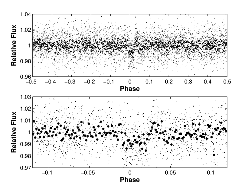
Figure 1.— The top panel shows the unbinned HATNet light curve with $6884$ data points, phased with the orbital period of $P=3.92289$ d. The binned light curve is over-plotted. The center of the transit is at phase zero. The bottom panel shows a zoom-in around the transit. The HATNet light curve is folded with the ephemeris obtained here, based on the follow-up light curves (see § 2.4). The small offset between phase zero and transit center suggests there is a slight difference in the ephemeris for the HATNet data and the photometric follow-up data, obtained $\sim 1000$ days apart. See § 7 for further discussion.

HAT-P-9 is positioned in HATNet’s internally labeled field G176, centered at $\alpha=07^{\mathrm{h}}28^{\mathrm{h}}$, $\delta=37\arcdeg 30\arcmin$. This field was observed in network mode by the HAT-6 telescope, located at the Fred Lawrence Whipple Observatory (FLWO) of the Smithsonian Astrophysical Observatory (SAO), and the HAT-9 telescope at the Submillimeter Array (SMA) site atop Mauna Kea, Hawaii. In total, $6884$ exposures were obtained at a 5.5 minute cadence between 2004 November 26 and 2005 October 21 (UT).

Preliminary reduction included standard bias, dark and flat-field corrections, followed by an astrometric solution using the code of Pál & Bakos (2006). Photometry was applied using fine-tuned aperture photometry while the raw light curves were processed by our external parameter decorrelation technique. Next, the Trend Filtering Algorithm (TFA; Kovács, Bakos, & Noyes, 2005) was applied to get the final light curves. To search for the signature of a transiting planet in the light curves we used the Box Least Squares (BLS; Kovács, Zucker, & Mazeh, 2002) algorithm.

A transit-like signal was identified in the light curve of HAT-P-9 (GSC 02463-00281, 2MASS J07204044+3708263), which is a $V$=12.3 mag star, fainter than most transiting planet host stars detected with small-aperture, wide-field, ground-based campaigns. The HATNet light curve is presented at the top panel of Fig. 1, folded on the ephemeris obtained from analyzing the follow-up light curves ($P$ = 3.92289 days and $T_{\rm c}=2454417.9077$, see § 2.4), showing a flux decrement of $\sim 1\,\%$ at phase zero. The figure shows a small shift between phase zero and transit center, suggesting a possible slight difference in the ephemeris for the HATNet data and the photometric follow-up data, obtained $\sim 1000$ days apart (see § 7 for further discussion). This transiting planet candidate, along with others from the same field, was selected for follow-up observations, to investigate its nature.

2.2. Early spectroscopy follow-up

Initial follow-up observations were made with the CfA Digital Speedometer (DS; Latham, 1992) in order to characterize the host star and to reject obvious astrophysical false-positive scenarios that mimic planetary transits. The five radial velocity (RV) measurements obtained over an interval of 62 days showed an rms residual of 1.1 $\rm km\,s^{-1}$, consistent with no detectable RV variation. Atmospheric parameters for the star (effective temperature $T_{\rm eff}$, surface gravity $\log g$, and projected rotational velocity $v\sin i$) were derived as described by Torres, Neuhäuser & Guenther (2002), initially assuming a fixed metallicity of [Fe/H] $=0.0\pm 0.2$. We obtained $\log g=4.05\pm 0.30$, $T_{\rm eff}=6130\pm 150$ K and $v\sin{i}=12.2\pm 1.0$ $\rm km\,s^{-1}$. As the DS results were consistent with a planet orbiting a moderately-rotating main sequence star, this target was selected for high-precision spectroscopy follow-up.

2.3. High-precision spectroscopy follow-up

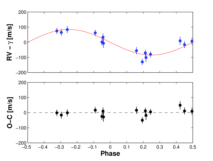
Figure 2.— The top panel shows the RV measurements phased with the period of $P=3.92289$ days and mid-transit time of $T_{\rm c}=2454417.9077$ (HJD). The zero-point in phase corresponds to the epoch of mid-transit. Overlaid is the best sinusoidal fit. The bottom panel shows the residuals from the fit.

Table 1 Radial Velocities for HAT-P-9.

BJD $-2,\!400,\!000$	RV	$\sigma_{\rm RV}$	BS	S/N
(days)	($\rm m\,s^{-1}$)	($\rm m\,s^{-1}$)	($\rm m\,s^{-1}$)
54233.3347	22667	24	-62	43
54379.6357	22586	20	5	44
54380.6213	22672	24	-93	38
54381.5815	22749	23	-148	40
54413.6292	22727	21	3	43
54414.6084	22610	24	-31	38
54415.6457	22675	27	-45	34
54416.6392	22740	21	-13	42
54421.6701	22659	31	-11	32
54422.6651	22595	20	-59	46
54587.3543	22536	21	10	44
54588.3571	22650	23	30	41
54589.3525	22730	23	-2	40
54590.3425	22699	25	-45	38
54591.3647	22564	30	10	32

Observations were carried out at the Haute Provence Observatory (OHP) 1.93-m telescope, with the SOPHIE spectrograph (Bouchy & the Sophie Team, 2006). SOPHIE is a multi-order echelle spectrograph fed through two fibers, one of which is used for starlight and the other for sky background or a wavelength calibration lamp. The instrument is entirely computer-controlled and a standard data reduction pipeline automatically processes the data upon CCD readout. RVs are calculated by numerical cross-correlation with a high resolution observed spectral template of a G2 star.

HAT-P-9 was observed with SOPHIE in the high-efficiency mode (R $\sim 39000$) during three observing runs, from 2007 May until 2008 May. Due to the relative faintness of this star, exposure times were in the range of 25 to 75 minutes, depending on observing conditions. The resulting signal to noise ratios were 32–46 per pixel at $\lambda=5500$ Å. Using the empirical relation of Cameron et al. (2007) we estimated the RV photon-noise uncertainties to be 20–31 $\rm m\,s^{-1}$. We made 17 RV measurements in total. Two of those were highly contaminated by the Moon and were ignored, leaving 15 RV measurements, listed in Table 1.

2.4. Photometry follow-up

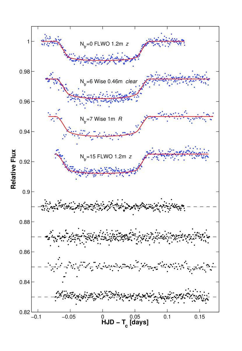
Figure 3.— Follow-up light curves of HAT-P-9. The four light curves are shown at the top of the figure, with the fitted model over-plotted. The label next to each light curve gives the transit event number, observatory, telescope and filter used. Residuals are presented at the bottom of the figure, with the same top to bottom order as the actual light curves.

Table 2 List of follow-up light curves of HAT-P-9.

$N_{\mathrm{tr}}$	Start Date	Observatory+	Filter	$u_{1}$	$u_{2}$	Cadence	$\beta$	RMS
	UT	Telescope				min-1		$\%$
0	2007 Nov 13	FLWO 1.2 m	$z$	0.1313	0.3664	1.0	1.1	0.17
6	2007 Dec   6	Wise 0.46 m	clear	0.2403	0.3816	1.1	1.0	0.21
7	2007 Dec  10	Wise 1.0 m	$R$	0.2403	0.3816	0.4	1.2	0.22
15	2008 Jan  11	FLWO 1.2 m	$z$	0.1313	0.3664	1.0	1.6	0.18

In order to better characterize the transit parameters and to derive a better ephemeris, we performed photometric follow-up observations with 1-m class telescopes. We obtained a total of four transit light curves of HAT-P-9b, shown in Fig. 3. Two events were observed by the KeplerCam detector on the FLWO 1.2 m telescope (see Holman et al., 2007) on UT 2007 Nov 13 and UT 2008 Jan 11, in the Sloan $z$-band. We refer to the 2007 Nov 13 event as having a transit number $N_{\mathrm{tr}}=0$, so the 2008 Jan 11 transit number is $N_{\mathrm{tr}}=15$. In addition, two light curves were obtained at the Wise Observatory. On UT 2007 Dec 6 the $N_{\mathrm{tr}}=6$ transit event was observed by the Wise 0.46 m telescope (Brosch et al., 2008), with no filter. The following event, with $N_{\mathrm{tr}}=7$, was observed on UT 2007 Dec 10 by the Wise 1 m telescope in the Cousins $R$-band. An additional light curve, obtained with the FLWO 1.2 m telescope, was of poor quality and is not included here. Table 2 lists for each light curve its $N_{\mathrm{tr}}$ number, UT date, observatory, telescope, filter used, limb-darkening coefficients used in its analysis, mean cadence, the correlated noise $\beta$ factor (see below) and the RMS residuals from the fitted light curve model.

Data were reduced in a similar manner to the HATNet data, using aperture photometry and an ensemble of $\sim$100 comparison stars in the field. An analytic model was fitted to these data, as described below in § 6, and yielded a period of $3.92289\pm 0.00004$ d and a reference epoch of mid-transit $T_{\mathrm{c}}=2,\!454,\!417.9077\pm 0.0003$ d (HJD). The length of the transit as determined from this joint fit is $0.143\pm 0.004$ d (3 hours, 26 minutes), the length of ingress is $0.019\pm 0.003$ d (27 minutes), and the central transit depth is $1.17\pm 0.01$ %. The latter value is simply the square of the radius ratio (see Table 4) if one ignores the limb-darkening effect. This effect increases the depth by about $0.1$ %, in the bands used here.

3. Stellar parameters

Table 3 Summary of stellar parameters for HAT-P-9.

Parameter	Value	Source
R.A.	$07^{\mathrm{h}}\,20^{\mathrm{m}}\,40.^{\mathrm{\!\!s}}44$	2MASS
Dec.	$+37\arcdeg\,08\arcmin\ \ 26.{\!\arcmin}3$	2MASS
$m_{V}$ (mag)	$12.297\pm 0.063$	TASS
$T_{\rm eff}$ (K)	$6350\pm 150$	DS + Yonsei-Yale
$v\sin{i}$ ($\rm km\,s^{-1}$)	$11.9\pm 1.0$	DS + Yonsei-Yale
$\log{g}$	$4.29^{+0.03}_{-0.04}$	DS + Yonsei-Yale + light curve shape
[Fe/H] (dex)	$0.12\pm 0.20$	DS + Yonsei-Yale
Mass ($M_{\sun}$)	$1.28\pm 0.13$	Yonsei-Yale + light curve shape
Radius ($R_{\sun}$)	$1.32\pm 0.07$	Yonsei-Yale + light curve shape
$\log(L_{\star}/L_{\sun})$	$0.41_{-0.09}^{+0.08}$	Yonsei-Yale
$M_{V}$ (mag)	$3.7^{+0.3}_{-0.2}$	Yonsei-Yale
Age (Gyr)	$1.6^{+1.8}_{-1.4}$	Yonsei-Yale + light curve shape
B-V (mag)	$0.50^{+0.06}_{-0.05}$	Yonsei-Yale
Distance (pc)	$480\pm 60$	Yonsei-Yale

The mass ($M_{p}$) and radius ($R_{p}$) of a transiting planet, determined from transit photometry and RV data, is dependent also on those of the parent star. In order to determine the stellar properties needed to place $M_{p}$ and $R_{p}$ on an absolute scale, we made use of stellar evolution models along with the observational constraints from spectroscopy and photometry, as described in Torres et al. (2008). Because of its relative faintness, the host star does not have a parallax measurement from Hipparcos, and thus a direct estimate of the absolute magnitude is not available for use as a constraint. An alternative approach is to use the surface gravity of the star, which is a measure of the evolutionary state of the star and therefore has a very strong influence on the radius. However, $\log{g}$ is a difficult quantity to measure spectroscopically and is often strongly correlated with other spectroscopic parameters (see § 2.2). It has been pointed out by Sozzetti et al. (2007) that the normalized separation of the planet, $a/R_{\star}$, can provide a much better constraint for stellar parameter determination than the spectroscopic $\log{g}$. The $a/R_{\star}$ quantity can be determined directly from the photometric observations with no additional assumptions (other than the values of the parameters describing limb-darkening, which is a second-order effect), and it is related to the mean density of the host star. As discussed later in § 6, an analytic fit to the light curve yields $a/R_{\star}$ = $8.6\pm 0.2$. This value, along with $T_{\rm eff}$ from § 2.2, and assuming [Fe/H] = $0.0\pm 0.2$, was compared with the Yonsei-Yale stellar evolution models of Yi et al. (2001). This resulted in values for the stellar mass and radius of $M_{\star}$= $1.16_{-0.15}^{+0.12}\,M_{\sun}$ and $R_{\star}$= $1.28\pm 0.08\,R_{\sun}$, and an estimated age of $3.6_{-2.2}^{+3.3}$ Gyr. The result for $\log{g}$ was $4.29^{+0.03}_{-0.04}$, consistent with the value derived from the DS spectra.

Nevertheless, in order to verify the overall consistency of our results and refine the stellar parameters, we carried out a new iteration. We imposed this latter value of $\log{g}$ (coming from stellar evolution modeling), and analyzed the DS spectra by allowing the metallicity, $v\sin{i}$ and $T_{\rm eff}$ to vary. The new results were [Fe/H] = $0.12\pm 0.20$, $v\sin{i}$ = $11.9\pm 1.0$ $\rm km\,s^{-1}$ and $T_{\rm eff}$ = $6350\pm 150$ K. Repeating the stellar evolution modeling resulted in $M_{\star}$= $1.28\pm 0.13$ $M_{\sun}$, $R_{\star}$= $1.32\pm 0.07$ $R_{\sun}$ and an age of $1.6^{+1.8}_{-1.4}$ Gyr. The stellar properties are summarized in Table 3 and they correspond to a late F star.

We used also our SOPHIE high-resolution spectra to estimate $v\sin{i}$ and [Fe/H]. Based on our result for $B-V$ from the stellar evolution models, of $B-V~{}=~{}$$0.50^{+0.06}_{-0.05}$ mag, we got $v\sin{i}$ = $10.1\pm 1.0$ $\rm km\,s^{-1}$ and [Fe/H]= $+0.18\pm 0.10$ dex. Those values are close to the results from the DS spectra and the stellar evolution model. However, the SOPHIE spectra were taken in High-Efficiency mode, where there is a known problem with removing the echelle blaze function. Hence, these estimates are used only for comparison, and are not included in our final result.

To check our spectroscopically determined $T_{\rm eff}$ we used several publicly available color indices for this star, and the calibrations of Ramírez & Meléndez (2005) and Casagrande et al. (2006) to derive independent temperature estimates, using the [Fe/H] value found above in these calibrations. We adjusted the reddening till the photometric temperature matched the spectroscopic temperature, yielding $E(B-V)=0.053$ (Ramírez & Meléndez, 2005) and $E(B-V)=0.043$ (Casagrande et al., 2006). We adopted the mean value of $0.048$ as reddening, implying an extinction of $A(V)=0.15$ mag. Note that the Burstein & Heiles (1982) reddening maps for this celestial position ($l,b$ = 181.1, 21.4) give $E(B-V)=0.072$ and the Schlegel et al. (1998) maps yield $E(B-V)=0.065$, broadly consistent with our findings, especially if we take into account that these latter methods measure the total reddening along the line of sight.

Using the $V$ magnitude from the TASS survey (Droege et al., 2006), $V$ = $12.297\pm 0.063$ mag, the absolute $V$ magnitude from the stellar evolution model, and the $A(V)=0.15$ mag value determined above, the distance to HAT-P-9 is $480\pm 60$ pc.

4. Spectroscopic orbital solution

Our 15 RV measurements from SOPHIE were fitted with a Keplerian orbit model solving for the velocity semi-amplitude $K$ and the center-of-mass velocity $\gamma$, holding the period and transit epoch fixed at the well-determined values from photometry (see Table 4). The eccentricity was initially set to zero. The fit yields $K=84.7\pm 7.9\,\rm m\,s^{-1}$ and $\gamma=22.665\pm 0.006\,\rm km\,s^{-1}$. The observations and fitted RV curve are displayed in the top panel of Fig. 2. The residuals are presented in the bottom panel of the same figure. RMS residuals is 22.1 $\rm m\,s^{-1}$, consistent with the RV uncertainties. The value of $\chi^{2}$ is 12.4 for 13 degrees of freedom.

5. Excluding blend scenarios

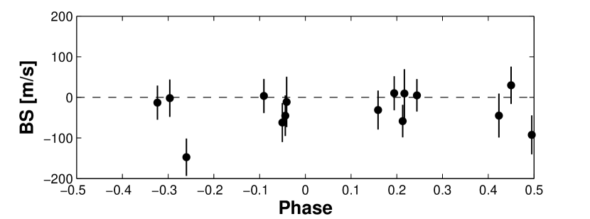
Figure 4.— Line bisector spans folded on the orbital phase. Albeit one or two outliers, the bisector spans do not show a variation with the orbital phase.

We tested the reality of the velocity variations by examining the spectral line bisector spans (BSs) of the star using our SOPHIE data. If the measured velocity changes are due only to distortions in the line profiles arising from contamination of the spectrum by the presence of a binary with a period of 3.92 days, we would expect the BSs (which measure line asymmetry) to vary with this period, resulting in a correlation between BS and RV (see, e.g., Queloz et al., 2001; Torres et al., 2005). As shown in Fig. 4, the BSs show no significant variations, except one or two outliers. The correlation coefficient between BS and RV for all 15 measurements is -0.38. Ignoring the extreme point reduces the correlation to -0.18.

In order to estimate the statistical significance of a correlation between BS and RV we define the following statistics:

$$r_{\sigma}=\frac{\sigma_{BS,fit}}{\sigma_{BS}},$$ (1)

where $\sigma_{BS}$ is the standard deviation of the BS values and $\sigma_{BS,fit}$ the standard deviation of the residuals of a BS fit to the RVs. Both standard deviations are the unbiased estimators. For pure noise $r_{\sigma}$ will equal 1.0. When fitting the BSs to the RVs of all 15 measurements, using polynomials of degrees 1–3 we got $r_{\sigma}$ in the range 0.984–1.043, consistent with no significant correlation.

Another sign of a binary would be a dependence between the RV amplitude and the template used. This may happen when the components of the blended binary are of a different spectral type than the primary target. We re-calculated the RVs using F0 and K5 templates and got an amplitude consistent with our original value, within $1\sigma$ (not shown).

These analyses indicate that the orbiting body is a planet with high significance.

6. Planetary parameters

Table 4 Orbital fit and planetary parameters for the HAT-P-9b system.

Parameter	Value
Ephemeris:
Period (day)	$3.92289\pm 0.00004$
$T_{\mathrm{c}}$ (HJD)	$2,\!454,\!417.9077\pm 0.0003$
Transit duration (day)	$0.143\pm 0.004$
Ingress duration (day)	$0.019\pm 0.003$
Orbital parameters:
$\gamma$ ($\rm km\,s^{-1}$)	$22.665\pm 0.006$
$K$ ($\rm m\,s^{-1}$)	$84.7\pm 7.9$
$e$	$0$
Light curve parameters:
$a/R_{\star}$	$8.6\pm 0.2$
$R_{p}/R_{\star}$	$0.1083\pm 0.0005$
$b$	$0.52\pm 0.03$
Planetary parameters:
$i$ (deg)	$86.5\pm 0.2$
$a$ (AU)	$0.053\pm 0.002$
$M_{p}$ ($M_{\rm J}$)	$0.78\pm 0.09$
$R_{p}$ ($R_{\rm J}$)	$1.40\pm 0.06$
$\rho_{p}$ ($\rm g\,cm^{-3}$)	$0.35\pm 0.06$
$g_{p}$ ($\rm m\,s^{-2}$)	$9.8\pm 1.0$
$T_{\rm eq}$ (K)	$1530\pm 40$
$\Theta$	$0.046\pm 0.007$
$f_{p}$ (109 erg cm-2 s-1)	$1.3^{+0.3}_{-0.3}$

To determine the light curve parameters of HAT-P-9b we fitted the four available transit light curves simultaneously, as described in Shporer et al. (2008). A circular orbit was assumed. We adopted a quadratic limb-darkening law for the star, and determined the appropriate coefficients, $u_{1}$ and $u_{2}$, by interpolating on the Claret (2000, 2004) grids for the atmospheric model described above. For the Wise 0.46 m light curve, observed with no filter, we adopted the Cousins $R$-band limb-darkening coefficients as the CCD response resembles a “wide-R” filter (Brosch et al., 2008). The values of the limb-darkening coefficients used for each light curve are listed on Table 2.

The drop in flux in the light curves was modeled with the formalism of Mandel & Agol (2002). The five adjusted parameters in the fit were i) the period $P$; ii) the mid-transit time of the $N_{tr}=0$ transit event, $T_{\mathrm{c,0}}$, denoted simply as $T_{\mathrm{c}}$; iii) the relative planetary radius, $r\equiv R_{p}/R_{\star}$; iv) the orbital semi-major axis scaled by the stellar radius, $a/R_{\star}$; v) the impact parameter, $b\equiv a\cos(i)/R_{\star}$, where $i$ is the orbital inclination angle.

Accounting for correlated noise in the photometric data (Pont et al., 2006) was done similarly to the “time-averaging” method of winn08. After a preliminary analysis we binned the residual light curves using bin sizes close to the duration of ingress and egress, which is 27 minutes. The presence of correlated noise in the data was quantified as the ratio between the standard deviation of the binned residual light curve and the expected standard deviation assuming pure white noise. This ratio is calculated separately for each bin size and we defined $\beta$ to be the largest ratio among the bin sizes we used. For each light curve we multiplied the relative flux errors by $\beta$ and repeated the analysis. The $\beta$ value of each light curve is listed on Table 2.

We used the Markov Chain Monte Carlo algorithm (MCMC, see, e.g. Holman et al., 2007) to derive the best fit parameters and their uncertainties. The MCMC algorithm results in a distribution of each of the fitted parameters. We took the distribution median to be the best fit value and the values at 84.13 and 15.87 percentiles to be the +1 $\sigma$ and -1 $\sigma$ confidence limits, respectively.

Our four follow-up light curves are presented in Fig. 3 where the fitted model is overplotted and the residuals are also shown. The result for the radius ratio is $R_{p}/R_{\star}=0.1083\pm 0.0005$, and the normalized separation is $a/R_{\star}=8.6\pm 0.2$. From the mass of the star (Table 3), the orbital parameters (§ 4) and the light curve parameters, the physical planetary parameters (such as mass, radius) are calculated in a straightforward way, and are summarized in Table 4. We note that $a/R_{\star}$, as derived from the light curve fit, is an important constraint for the stellar parameter determination (§ 3), which in turn defines the limb-darkening coefficients that are used in the light curve analytic fit. Thus, after the initial analytic fit to the light curves and the stellar parameter determination, we performed another iteration of the light curve fit. We found that the change in parameters was imperceptible.

7. Discussion

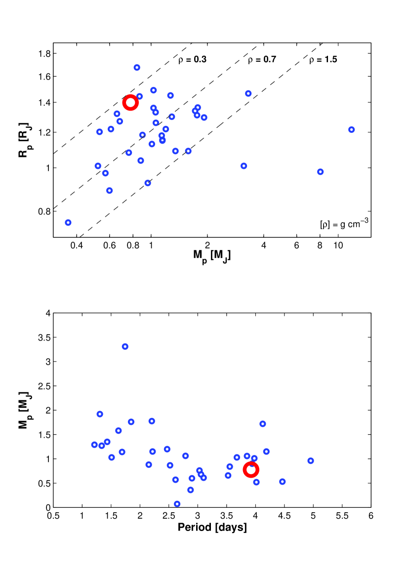
Figure 5.— Top panel: The radius-mass diagram for the known transiting planets, in log-log scale, with HAT-P-9b marked by an open circle. Constant density lines are over-plotted. The diagram visually shows that the new planet has a relatively low density. The Neptune-mass planet GJ 436b, orbiting an M star, is positioned beyond the lower-left corner of this diagram.
Bottom panel: The mass-period diagram for the known transiting planets, in linear scale, with HAT-P-9b marked by an open circle. Three planets are positioned outside the boundaries of this diagram: The long-period planet HD 17156b, and the massive planets HAT-P-2b (a.k.a. HD 147506b) and XO-3b. The planet with the lowest mass in this diagram is GJ 436b, orbiting an M star, and the one with the largest mass is CoRoT-Exo-2b.
This figure is based on data taken from http://www.inscience.ch/transits/ on 2008 June 1st.

We present here the discovery of a new transiting extra-solar planet, HAT-P-9b, with a mass of $0.78\pm 0.09$ $M_{\rm J}$, radius of $1.40\pm 0.06$ $R_{\rm J}$ and orbital period of $3.92289\pm 0.00004$ days. The $V=12.3$ mag host star is among the faintest planet-host stars identified with small-aperture, wide-field, ground-based campaigns. In fact, together with WASP-5 (Anderson et al., 2008) they are currently the faintest planet-host stars discovered with such campaigns, where the transit depth is below 2%.

To show the main characteristics of the new planet relative to the currently known transiting planets we plot in Fig. 5 the position of the latter on the radius-mass diagram, on the top panel, and the mass-period diagram, on the bottom panel. In both panels HAT-P-9b position is marked by an open circle.

The radius-mass diagram, presented here in log-log scale, visually shows that the new planet has a low density, of $\rho_{p}$= $0.35\pm 0.06$ $\rm g\,cm^{-3}$, similar to that of HD 209458b (e.g., Knutson et al., 2007; Mazeh et al., 2000), WASP-1b (Cameron et al., 2007; Shporer et al., 2007; Charbonneau et al., 2007), HAT-P-1b (Bakos et al., 2007; Winn et al., 2007b) and CoRoT-Exo-1b (Barge et al., 2008).

Comparing the measured radius to the modeled radius of Burrows et al. (2007), for the same stellar luminosity, semi-major axis and (core-less) planet mass as the HAT-P-9 system, shows the measured value is larger than the modeled one by 1-2 $\sigma$. In this comparison we assumed solar opacity for the planetary atmosphere. As shown by Burrows et al. (2007), the transit radius effect together with enhanced planetary atmospheric opacities, relative to solar opacity, can be responsible for inflating the planetary radius. Since atmospheric opacities are related to the host star metallicity, and HAT-P-9 metallicity seems to be super-solar, it is likely that these two effects account for the radius difference, as is the case for WASP-1b (Burrows et al., 2007, see their Fig. 7). Other mechanisms that may explain the increased radius involve downward transport and dissipation of kinetic energy (Showman & Guillot, 2002) and layered convection (Chabrier & Baraffe, 2007).

According to its $T_{\rm eq}$ and Safronov number, listed on Table 4, HAT-P-9b is likely a Class II planet, as defined by Hansen & Barman (2007). This classification is in accordance with its low density, since members of this class usually have smaller masses and larger radii than those of Class I.

The stellar incident flux at the planet is $f_{p}$ = $1.3^{+0.3}_{-0.3}$ 10⁹ erg cm^-2 s^-1, which is at the lower end of the $f_{p}$ range for pM planets, according to the pL/pM planet classification of Fortney et al. (2008b). Since it is positioned near the transition region in $f_{p}$ between these two classes of planets it may be used to further characterize them.

In the mass-period diagram the new planet is positioned near XO-1b (McCullough et al., 2006; Holman et al., 2006), OGLE-TR-182b (Pont et al., 2008), OGLE-TR-111b (Pont et al., 2004; Winn et al., 2007a) and HAT-P-6b (Noyes et al., 2008). The position of HAT-P-9b, along with that of neighbouring planets, suggests that the mass-period relation (Mazeh, Zucker, & Pont, 2005; Gaudi et al., 2005), i.e., the decrease of planetary mass with increasing orbital period, levels-off at periods $\gtrsim 3$ days.

The ephemeris obtained here is based on the four follow-up light curves. We compared it to the mid-transit time of the HATNet light curve, obtained some 1000 days earlier, by propagating the error on the period. The result shows a difference of about 1.5 $\sigma$ between the mid-transit times of the follow-up light curves and that of the HATNet light curve. Future follow-up light curves will be able to study more thoroughly this possible discrepancy.

Finally, we note that due to the line-of-sight stellar rotation velocity of $11.9\pm 1.0$ $\rm km\,s^{-1}$ and the non-zero impact parameter $0.52\pm 0.03$, this planet is a good candidate for the measurement of the Rossiter-Mclaughlin effect (e.g., Winn et al., 2005). Eq. 6 of Gaudi & Winn (2007) gives an expected amplitude for the effect of more than 100 $\rm m\,s^{-1}$, which is larger than the orbital amplitude. However, since this is a relatively faint star, with $V=12.3$ mag, such a measurement will be challenging.

References

- Anderson et al. (2008) Anderson, D. R., et al. 2008, MNRAS, 387, L4
- Bakos et al. (2002) Bakos, G. Á., Lázár, J., Papp, I., Sári, P., & Green, E. M. 2002, PASP, 114, 974
- Bakos et al. (2004) Bakos, G. Á., Noyes, R. W., Kovács, G., Stanek, K. Z., Sasselov, D. D., & Domsa, I. 2004, PASP, 116, 266
- Bakos et al. (2007) Bakos, G. Á., et al. 2007, ApJ, 656, 552
- Baraffe et al. (2008) Baraffe, I., Chabrier, G., & Barman, T. 2008, A&A, 482, 315
- Barge et al. (2008) Barge, P., et al. 2008, A&A, 482, L17
- Bouchy & the Sophie Team (2006) Bouchy, F., & The Sophie Team 2006, Tenth Anniversary of 51 Peg-b: Status of and prospects for hot Jupiter studies, 319
- Brosch et al. (2008) Brosch, N., Polishook, D., Shporer, A., Kaspi, S., Berwald, A., & Manulis, I. 2008, Ap&SS, 314, 163
- Burrows et al. (2007) Burrows, A., Hubeny, I., Budaj, J., & Hubbard, W. B.2007, ApJ, 661, 502
- Burrows et al. (2008) Burrows, A., Budaj, J.,& Hubeny, I. 2008, ApJ, 678, 1436
- Burstein & Heiles (1982) Burstein, D., & Heiles, C. 1982, AJ, 87, 1165
- Cameron et al. (2007) Cameron, A. C., et al. 2007, MNRAS, 375, 951
- Casagrande et al. (2006) Casagrande, L.,Portinari, L., & Flynn, C. 2006, MNRAS, 373, 13
- Chabrier & Baraffe (2007) Chabrier, G., & Baraffe, I. 2007, ApJ, 661, L81
- Charbonneau et al. (2007) Charbonneau, D., Winn, J. N., Everett, M. E., Latham, D. W., Holman, M. J., Esquerdo, G. A., & O’Donovan, F. T. 2007, ApJ, 658, 1322
- Claret (2000) Claret, A. 2000, A&A, 363, 1081
- Claret (2004) Claret, A. 2004, A&A, 428, 1001
- Droege et al. (2006) Droege, T. F., Richmond,M. W., Sallman, M. P., & Creager, R. P. 2006, PASP, 118, 1666
- Fortney (2008a) Fortney, J. J. 2008a, ArXiv e-prints, arXiv:0801.4943
- Fortney et al. (2008b) Fortney, J. J., Lodders, K., Marley, M. S., & Freedman, R. S. 2008b, ApJ, 678, 1419
- Gaudi et al. (2005) Gaudi, B. S., Seager, S., & Mallen-Ornelas, G. 2005, ApJ, 623, 472
- Gaudi & Winn (2007) Gaudi, B. S., & Winn, J. N. 2007, ApJ, 655, 550
- Guillot et al. (2006) Guillot, T., Santos, N. C., Pont, F., Iro, N., Melo, C., & Ribas, I. 2006, A&A, 453, L21
- Hansen & Barman (2007) Hansen, B. M. S., & Barman, T. 2007, ApJ, 671, 861
- Holman et al. (2006) Holman, M. J., et al. 2006, ApJ, 652, 1715
- Holman et al. (2007) Holman, M. J., et al. 2007, ApJ, 664, 1185
- Knutson et al. (2007) Knutson, H. A., Charbonneau, D., Noyes, R. W., Brown, T. M., & Gilliland, R. L. 2007, ApJ, 655, 564
- Kovács, Zucker, & Mazeh (2002) Kovács, G., Zucker, S., & Mazeh, T. 2002, A&A, 391, 369
- Kovács, Bakos, & Noyes (2005) Kovács, G., Bakos, G. Á., & Noyes, R. W. 2005, MNRAS, 356, 557
- Latham (1992) Latham, D. W. 1992, ASP Conf. Ser. 32: IAU Colloq. 135: Complementary Approaches to Double and Multiple Star Research, 32, 110
- Mazeh et al. (2000) Mazeh, T., et al. 2000, ApJ, 532, L55
- Mandel & Agol (2002) Mandel, K., & Agol, E. 2002, ApJ, 580, L171
- Mazeh, Zucker, & Pont (2005) Mazeh, T., Zucker, S., & Pont, F. 2005, MNRAS, 356, 955
- McCullough et al. (2006) McCullough, P. R., et al. 2006, ApJ, 648, 1228
- Minniti et al. (2007) Minniti, D., et al. 2007, ApJ, 660, 858
- Noyes et al. (2008) Noyes, R. W., et al. 2008, ApJ, 673, L79
- Pál & Bakos (2006) Pál, A., & Bakos, G. Á. 2006, PASP, 118, 1474
- Pont et al. (2004) Pont, F., Bouchy, F., Queloz, D., Santos, N. C., Melo, C., Mayor, M., & Udry, S. 2004, A&A, 426, L15
- Pont et al. (2006) Pont, F., Zucker, S., & Queloz, D. 2006, MNRAS, 373, 231
- Pont et al. (2008) Pont, F., et al. 2008, A&A, 487, 749
- Queloz et al. (2001) Queloz, D. et al. 2001, A&A, 379, 279
- Ramírez & Meléndez (2005) Ramírez, I., & Meléndez, J. 2005, ApJ, 626, 465
- Schlegel et al. (1998) Schlegel, D. J., Finkbeiner, D. P., & Davis, M. 1998, ApJ, 500, 525
- Showman & Guillot (2002) Showman, A. P., & Guillot, T. 2002, A&A, 385, 166
- Shporer et al. (2007) Shporer, A., Tamuz, O., Zucker, S., & Mazeh, T. 2007, MNRAS, 376, 1296
- Shporer et al. (2008) Shporer, A., Mazeh, T., Winn, J. N., Holman, M. J., Latham, D. W., Pont, F., & Esquerdo, G. A. 2008, ApJ, submitted, arXiv:0805.3915
- Southworth et al. (2007) Southworth, J., Wheatley, P. J., & Sams, G. 2007, MNRAS, 379, L11
- Sozzetti et al. (2007) Sozzetti, A. et al. 2007, ApJ, 664, 1190
- Torres, Neuhäuser & Guenther (2002) Torres, G., Neuhäuser, R., & Guenther, E. W. 2002, AJ, 123, 1701
- Torres et al. (2005) Torres, G., Konacki, M., Sasselov, D. D., & Jha, S. 2005, ApJ, 619, 558
- Torres et al. (2008) Torres, G., Winn, J. N., & Holman, M. J. 2008, ApJ, 677, 1324
- Winn et al. (2005) Winn, J. N., et al. 2005, ApJ, 631, 1215
- Winn et al. (2007a) Winn, J. N., Holman, M. J., & Fuentes, C. I. 2007a, AJ, 133, 11
- Winn et al. (2007b) Winn, J. N., et al. 2007b, AJ, 134, 1707
- Winn et al. (2008) Winn, J. N., et al. 2008, ApJ, 683, 1076
- Yi et al. (2001) Yi, S. K. et al 2001, ApJS, 136, 417