Velocity-correlation distributions in granular systems

Abstract

We investigate the velocity-correlation distributions after $n$ collisions of a tagged particle undergoing binary collisions. Analytical expressions are obtained in any dimension for the velocity-correlation distribution after the first-collision as well as for the velocity-correlation function after an infinite number of collisions, in the limit of Gaussian velocity distributions. It appears that the decay of the first-collision velocity-correlation distribution for negative argument is exponential in any dimension with a coefficient that depends on the mass and on the coefficient of restitution. We also obtained the velocity-correlation distribution when the velocity distributions are not Gaussian: by inserting Sonine corrections of the velocity distributions, we derive the corrections to the velocity-correlation distribution which agree perfectly with a DSMC (Direct Simulation Monte Carlo) simulation. We emphasize that these new quantities can be easily obtained in simulations and likely in experiments: they could be an efficient probe of the local environment and of the degree of inelasticity of the collisions.

I Introduction

The dynamics of hard-core particles consists of successive binary collisions. For atomic systems, the equilibrium state can be reached, and is characterized by velocity distributions which are purely Gaussian. Conversely, in the presence of dissipation, i.e. for granular particles, no equilibrium exists, but when an external source of energy is present the system reaches a steady state whose properties can be compared to the equilibrium state of atomic systemsBP004 . At low to intermediate densities, spatial correlations are not responsible for non-Gaussian deviationsBaxter2007 .

The short-time dynamics is usually analyzed by means of the velocity autocorrelation function. This quantity provides an average of the scalar product of the velocity at time $0$ with the velocity at time $t$. The characteristic time of this correlation function corresponds to the time needed for the system to lose memory of the initial configuration of the velocities. Some progress has been made recently by investigating the collision statistics: Visco et. alVisco2008 ; Visco2008a showed that the free flight time distribution is not exponential, even in the low-density limit (such a behavior was observed in Molecular Simulation of hard spheres some years agoTalbot1992 ). Deviations from the Poisson law of the number of collisions can be captured in the framework of the Boltzmann equation and agree with molecular simulation results.

We introduce here a new quantity by focusing on collision events irrespective of the time when individual collisions occur. We consider the scalar product between the velocity before a given collision and the velocity after $n$ collisions. (Note that this quantity is distinct from the distribution of velocity for a hard sphere on collision, which characterizes the distribution of the relative velocity of colliding spheres, for which LueLue2005 obtained exact results in three, four and five dimensions). The information obtained is not only the average of the scalar product, but the full distribution of the scalar product between the velocity before and after a sequence of $n$ collisions. When $n=1$, this corresponds to the probability of the scalar product between the pre- and post-collisional velocities during a collision; it is worth noting that the first moment of the distribution does not correspond to the velocity correlation function at the mean collision time: indeed, the probability distribution is built for collisions occurring at different collision times, whereas the velocity correlation function corresponds to the velocities scalar product at a given time.

As the number of collisions increases, the correlations between velocities decrease and the distribution evolves progressively to the asymptotic form where the velocities are uncorrelated. The paper is organized as follows: in section II, we obtain the probability distributions in the limit of an infinite number of collisions, i.e. when the velocities are completely uncorrelated, in any spatial dimension. In section III, we derive the first-collision velocity distribution in any dimension. Section IV is devoted to the corrections induced by the non-Gaussian behavior of granular systems, and we compare the analytical results to DSMC results. Velocity-correlation distributions at the second and higher collisions are analyzed in Section V.

Let us define, right away, the central quantity of this study, the velocity-correlation distribution $P_{n}(z)$ at the $n$th collision :

$$P_{n}(z)=\langle\delta(z-{\bf v}.{\bf v}^{*}_{n})\rangle$$ (1)

where the brackets denote a statistical average in a given steady state, ${\bf v}$ denotes the precollisional velocity of a tagged particle before the first collision and ${\bf v}^{*}_{n}$ the postcollisional velocity of the same particle after the $n$th collision. We only consider the case of homogeneous systems.

II Velocity-correlation distribution in the infinite collision limit

We first consider the situation where the number of collisions is very large, i.e. the velocity before the first collision and the velocity after a large number of collisions become uncorrelated. The probability distribution of the scalar product $P_{\infty}(z={\bf v}.{\bf v^{*}}_{\infty})$ is then given by

$$P_{\infty}(z)=\int\int d{\bf v}d{\bf v^{*}_{\infty}}f({\bf v})f({\bf v^{*}}_{\infty})\delta(z-{\bf v}.{\bf v^{*}}_{\infty}).$$ (2)

Let us consider the generating function $\tilde{P}_{\infty}(k)=\int dke^{ikz}P_{\infty}(z)$. One has

$$\tilde{P}^{(d)}_{\infty}(k)=\int\int d{\bf v}d{\bf v^{*}}_{\infty}f({\bf v})f({\bf v^{*}}_{\infty})e^{ik{\bf v}.{\bf v^{*}}_{\infty}}.$$ (3)

We assume that the velocity distribution can be factorized as $f({\bf v})=\prod_{\alpha=1}^{d}f(v_{\alpha})$ where $\alpha$ is an index running over all components of the velocity and $d$ the space dimension. The Cartesian components of the velocity are independent random variables and the generating function is then also the product of the generating functions of each Cartesian component:

$$\tilde{P}_{\infty}^{(d)}(k)=(\tilde{P}^{(1)}_{\infty}(k))^{d},$$ (4)

where $\tilde{P^{(1)}_{\infty}}(k)$ is the generating function for the one-dimensional problem.

$P^{(1)}_{\infty}(z)$ can be obtained from Eq. (2), which gives

$$P^{(1)}_{\infty}(z)=\int\frac{dv}{|v|}f(z/v)f(v).$$ (5)

It is worth noting that ${P}^{(1)}_{\infty}$ is the Mellin convolution of the two velocity distributions as this distribution is that of the product of two independent random variables. When the velocity distribution $f(v)$ is Gaussian

$$f(v)=\sqrt{\frac{M}{2\pi T}}e^{-\frac{Mv^{2}}{2T}},$$ (6)

where $M$ and $T$ are the mass and the temperature of the tagged particle, respectively.

$P^{(1)}_{\infty}(z)$ can be explicitly obtained and is then equal to

$$P^{(1)}_{\infty}(z)=\frac{MK_{0}(\frac{|z|M}{T})}{\pi T},$$ (7)

where $K_{0}(z)$ is the modified Bessel function of second kind.

The basic property of ${P}^{(1)}_{\infty}$ is that the distribution is symmetric because the velocities are uncorrelated. The behavior of ${P}^{(1)}_{\infty}$ is intriguing at small values of $z$, as one observes a logarithmic divergence at $z=0$. This means that there is an overpopulated density of very small scalar products even though the velocity distribution remains finite for very small velocities. For large velocities, ${P}^{(1)}_{\infty}$ decays as $\exp(-|z|M/T)/\sqrt{z}$ for large values of $z$, i.e. less rapidly than the original velocity distribution which has a Gaussian decay.

In two and more dimensions, the velocity-correlation distribution can be obtained by noting that the Fourier transform of Eq.(7) (or integrating Eq.(3)), leads to

$$\tilde{P}^{(1)}_{\infty}(k)=\frac{1}{\sqrt{1+k^{2}}}.$$ (8)

By inserting Eq.(8) in Eq.(4), the generating function $\tilde{P}^{(d)}_{\infty}(k)$ in $d$ dimensions is then

$$\tilde{P}^{(d)}_{\infty}(k)=(1+k^{2})^{-d/2}.$$ (9)

The inverse Fourier transform can be calculated in any dimension: in 2D, the Fourier transform has a Lorentz profile, which gives in real space

$$P^{(2)}_{\infty}(z)=\frac{M\exp(-|z|M/T)}{2T},$$ (10)

and in three dimensions,

$$P_{\infty}^{(3)}(z)=z\frac{MK_{1}(\frac{|z|M}{T})}{\pi T}.$$ (11)

In 2D and in 3D, the probability distribution is no longer singular at the origin. However, there exists a non-analytic behavior which is a cusp in 2D and a cusp in the derivative in 3D.

For completeness, the solution in odd dimensions; $P^{(d)}_{\infty}(z)$ is given by

$$P^{(d)}_{\infty}(z)=\sqrt{\frac{2}{\pi}}|z|^{(d-1)/2}\frac{(d-2)!}{2^{(d-3)/2}((d-3)/2)!}K((d-1)/2,|z|)$$ (12)

collision where $K((d-1)/2,|z|)$ is the modified Bessel function of second kind of order $(d-1)/2$.

III First-collision velocity-correlation distribution

In order to have tractable expressions for the first-collision velocity-correlation distribution $P_{1}(z)$, we assume that the the “molecular chaos” is valid, i.e. that there are no correlations between the particles before collision. The joint velocity distribution of the tagged particle and the bath particles is simply the product of the individual velocity distributions. Moreover, it is necessary to account for the rate of collisions which depends on the relative velocity at the point of impact as well as all possibilities of collision by summing up on the locations of the impact on the sphere. $P_{1}(z)$ is then given by

$$P_{1}(z) =C\int_{S}\int\int d{\bf n}d{\bf u}d{\bf v}|({\bf v}-{\bf u}).{\bf n}|f({\bf v})$$

$$f_{B}({\bf u})\delta(z-{\bf v}.{\bf v^{*}}),$$ (13)

where $f(v)$ and $f_{B}({\bf u})$ are, respectively, the velocity distributions of the tagged and bath particles. The integral with the subscript $S$ corresponds to the integration over the unit sphere with the restriction $({\bf u}-{\bf v}).{\bf n}<0$ where ${\bf n}$ is a unit vector along the axis joining the two centers of particles (this imposes that the particles are approaching each other before colliding). $C$ is the normalization constant such that $\int_{-\infty}^{\infty}dzP_{1}(z)=1$.

The postcollisional velocity ${\bf v^{*}}$ is given by the collision rule which is

$${\bf v}^{*}={\bf v}+m\frac{1+\alpha}{m+M}[({\bf u}-{\bf v}).{\bf n}]{\bf n},$$ (14)

where $M$ and $m$ are, respectively, the mass of the tagged and of the bath particle . $\alpha$ is the normal restitution coefficient comprised between $0$ and $1$. For conveniencePuglisi2006 ; SD06 ; PTV06 , we introduce $\alpha^{\prime}$ such that

$$\frac{1+\alpha^{\prime}}{2}=m\frac{1+\alpha}{M+m}.$$ (15)

III.1 One dimension

In one dimension, the integral over angles is replaced by counting the right and left collisions. Therefore, Eq.(III) becomes

$$P^{(1)}_{1}(z)=C\int\int dudv|u-v|f(v)f_{B}(u)\delta(z-vv^{*}).$$ (16)

For granular gases, even if the velocity distributions of the tagged particle and of the bath particle are GaussianMP99 ; Garzo1999 (or close to the Gaussian profileBrey2005b ), the granular temperatures of these two species are always different when $\alpha<1$. Let us denote $\gamma$ the ratio between the bath and the tagged particle temperatures. The velocity distribution of the two species read :

$$f(v)=\sqrt{\frac{M}{2\pi T}}e^{-\frac{Mv^{2}}{2\gamma T}}$$ (17)

and

$$f_{B}(v)=\sqrt{\frac{m}{2\pi T}}e^{-\frac{mv^{2}}{2T}}.$$ (18)

It is necessary to distinguish the case $z<0$, where the distribution $P^{(1)}_{1}(z)$ is given by

$$P^{(1)}_{1}(z) =\frac{4C}{(1+\alpha^{\prime})^{2}}\int dv\left(1-\frac{z}{v^{2}}\right)f(v)\times$$

$$\times f_{B}\left(\frac{v(1-\alpha^{\prime})}{1+\alpha^{\prime}}-\frac{2z}{(1+\alpha^{\prime})v}\right)$$ (19)

from the case $z>0$, where $P^{(1)}_{1}(z)$ is equal to

$$P^{(1)}_{1}(z)= \frac{4C}{(1+\alpha^{\prime})^{2}}\left[\int_{0}^{\sqrt{z}}dv-\int_{\sqrt{z}}^{+\infty}\right]\left(\frac{z}{v^{2}}-1\right)f(v)\times$$

$$\times f_{B}\left(\frac{v(1-\alpha^{\prime})}{1+\alpha^{\prime}}-\frac{2z}{(1+\alpha^{\prime})v}\right).$$ (20)

Explicit integration over the velocity can be performed and some details of the calculation are given in Appendix A. Let us introduce

$$a =\sqrt{\frac{M}{\gamma T}+\frac{m}{T}\left(\frac{1-\alpha^{\prime}}{1+\alpha^{\prime}}\right)^{2}},$$ (21)

$$b =\sqrt{\frac{m}{T}\left(\frac{2}{1+\alpha^{\prime}}\right)^{2}},$$ (22)

$$c =\frac{2m}{T}\frac{1-\alpha^{\prime}}{(1+\alpha^{\prime})^{2}}.$$ (23)

the first-collision velocity-correlation distribution $P^{(1)}_{1}(z)$ then reads for $z<0$

$$P^{(1)}_{1}(z)=P^{(1)}_{1}(0)e^{(ab+c)z}$$ (24)

and for $z>0$

$$P^{(1)}_{1}(z) =P^{(1)}_{1}(0)e^{cz}\left(\frac{a-b}{a+b}e^{-abz}erf\left(\frac{a-b}{\sqrt{2}}\sqrt{z}\right)\right.$$

$$\left.+e^{abz}erfc\left(\frac{a+b}{\sqrt{2}}\sqrt{z}\right)\right),$$ (25)

where $P^{(1)}_{1}(0)$ is given by

$$P^{(1)}_{1}(0)=\frac{(a+b)(a^{2}b^{2}-c^{2})}{2ab\sqrt{a^{2}+b^{2}-2c}}.$$ (26)

Note that $P^{(1)}_{1}(z)$ is always asymmetric, contrary to an uncorrelated velocity distribution; this results from the existence of correlations between pre and post-collisional velocities of a particle. Secondly, $P^{(1)}_{1}(z)$ is finite when $z$ goes to $0$, which is not the case for $P^{(1)}_{\infty}(z)$.

To simplify the above expressions, Eq.(24)-(III.1) and to allow us to discuss the physical results, we now need to specify the temperature ratio $\gamma$. For inelastic particles in a polydisperse granular bath, $\gamma$ is in general a complicated function of parameters such as the bath composition, the heating mechanism and the coefficient of restitution. However, three interesting limiting cases provide a simple expression of the temperature ratio : (i) monodisperse system, for which $\gamma=1$ (in a Gaussian approximation);

(ii) a mixture of granular gases in the limit of infinite dilution. Martin and PiaseckiMP99 showed that the velocity distribution of an inelastic tracer in an elastic bath remains Gaussian with a granular temperature of the tracer given by the relation $T_{eff}=\gamma T_{bain}$ (equipartition does not hold); this ratio $\gamma$ is given by

$$\gamma=\frac{M}{m}\frac{1+\alpha^{\prime}}{3-\alpha^{\prime}}.$$ (27)

(iii) Thermalized systems of elastic particles ($\alpha=1$), $P^{(1)}_{1}(z)$ then provides a non trivial information on the short-time dynamics even for equilibrium systems.

In the first case ($M=m$ and $\gamma=1$), $\alpha^{\prime}=\alpha$. This gives for the first-collision velocity-correlation distribution, for $z<0$

$$P^{(1)}_{1}(z)=\frac{M}{T}\frac{2+\sqrt{2(1+\alpha^{2})}}{2(1+\alpha)\sqrt{1+\alpha^{2}}}e^{\frac{2}{(1+\alpha)^{2}}(\sqrt{2(1+\alpha^{2})}+1-\alpha)\frac{Mz}{T}}$$ (28)

and for $z>0$,

$$P^{(1)}_{1}(z)=\frac{M}{T}\frac{e^{\frac{2(1-\alpha)}{(1+\alpha)^{2}}\frac{Mz}{T}}}{2(1+\alpha)\sqrt{1+\alpha^{2}}}$$

$$\left[(2-\sqrt{2(1+\alpha^{2})})e^{-\frac{2}{(1+\alpha)^{2}}(\sqrt{2(1+\alpha^{2})})\frac{Mz}{T}}\right.$$

$$erf\left(\frac{\sqrt{2}-\sqrt{(1+\alpha^{2})}}{1+\alpha}\sqrt{\frac{Mz}{T}}\right)+$$

$$+(2+\sqrt{2(1+\alpha^{2})})e^{\frac{2}{(1+\alpha)^{2}}(\sqrt{2(1+\alpha^{2})})\frac{Mz}{T}}$$

$$\left.erfc\left(\frac{\sqrt{2}+\sqrt{(1+\alpha^{2})}}{1+\alpha}\sqrt{\frac{Mz}{T}}\right)\right].$$ (29)

The decay of $P^{(1)}_{1}(z)$ also depends on both the temperature on the coefficient of restitution $\alpha$.

In the second case (granular tracer in a thermalized bath), substituting Eq.(27) in Eqs.(21)-(22), one obtains that $a=b=\sqrt{\frac{m}{T}}\frac{2}{1+\alpha^{\prime}}$, which gives a simple expression for $P^{(1)}_{1}(z)$. For $z<0$

$$P^{(1)}_{1}(z)=\frac{m}{T}\frac{3-\alpha^{\prime}}{(1+\alpha^{\prime})^{3/2}}e^{\frac{3-\alpha^{\prime}}{(1+\alpha^{\prime})^{2}}\frac{2mz}{T}}.$$ (30)

and for $z>0$

$$P^{(1)}_{1}(z)=\frac{m}{T}\frac{3-\alpha^{\prime}}{(1+\alpha^{\prime})^{3/2}}e^{\frac{2m}{T}\frac{3-\alpha^{\prime}}{(1+\alpha^{\prime})^{2}}z}erfc\left(\frac{2}{1+\alpha^{\prime}}\sqrt{\frac{2mz}{T}}\right)$$ (31)

In order to show that the local environment influences the first-collision velocity-correlation distribution, we reexpress $P^{(1)}_{1}(z)$ in terms of the temperature of the tracer $\gamma T$. Substituting Eq.(27) in Eqs.(30)-(31), one obtains that for $z>0$ $P^{(1)}_{1}(z)=\frac{M}{\gamma T}\frac{1}{\sqrt{1+\alpha^{\prime}}}e^{\frac{1}{(1+\alpha^{\prime})}\frac{2Mz}{\gamma T}}$. Comparison with Eq.(28) shows that $P^{(1)}_{1}(z)$ is sensitive to the heating procedure, the temperature of the tracer particle being the same in both cases.

Finally, for elastic hard particles ($\alpha=1$), the equipartition holds, $\gamma=1$, and therefore Eqs.(21)-(23) become $a=b=(M+m)/(2\sqrt{mT})$ and $c=(M^{2}-m^{2})/(4mT)$, and $P^{(1)}_{1}(z)$ reads for $z<0$

$$P^{(1)}_{1}(z)=\frac{M}{2T}\sqrt{1+\frac{M}{m}}e^{\frac{M(M+m)}{2mT}z}$$ (32)

and for $z>0$

$$P^{(1)}_{1}(z)=\frac{M}{2T}\sqrt{1+\frac{M}{m}}e^{\frac{M(M+m)}{2mT}z}erfc\left((M+m)\sqrt{\frac{z}{2mT}}\right).$$ (33)

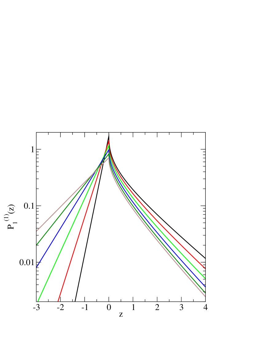
Figure 1: Log-linear plot of $P^{(1)}_{1}(z)$ versus $z$ ($M/T$ is set to $1$) (Eqs (28)- (III.1)).: Left, from top to bottom, the coefficient of restitution $\alpha=0,0.2,0.4,0.6,0.8,1$.

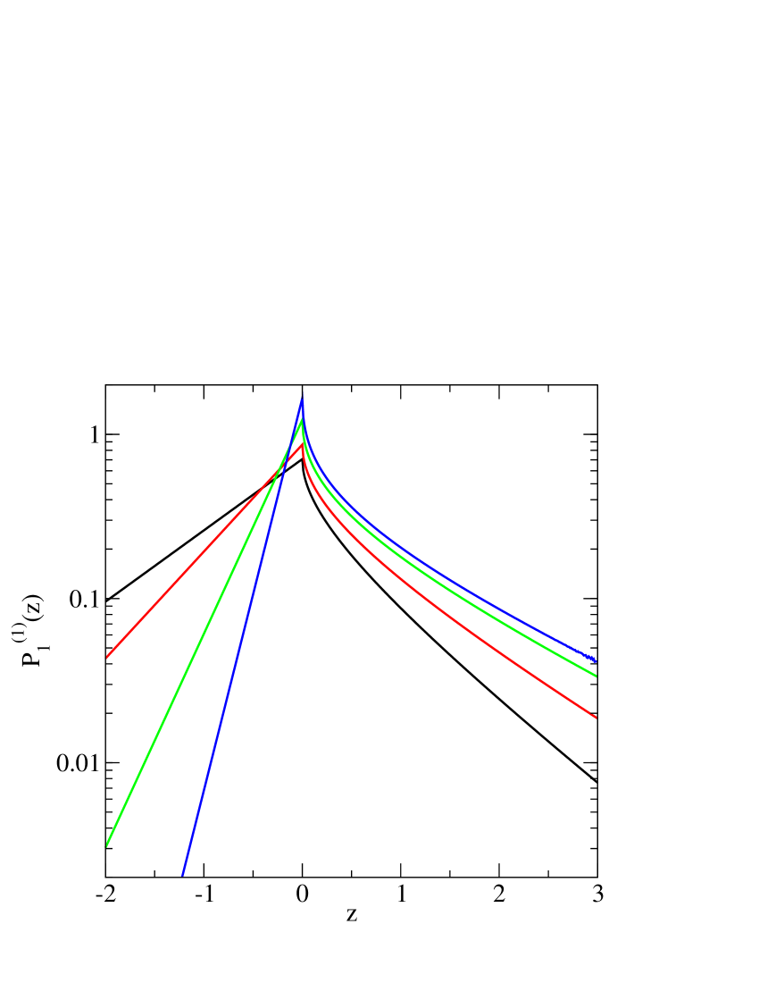
Figure 2: Log-linear plot of $P^{(1)}_{1}(z)$ versus $z$, for elastic hard spheres (Eqs.(32)- (33)). The mass ratios are $\frac{m}{M}=1,\frac{1}{2},\frac{1}{5},\frac{1}{10}$ (on the left side, from top curve to bottom curve).

Figure 1 displays $P^{(1)}_{1}(z)$ as a function of $z$ for different values of the coefficient of restitution $\alpha=0,0.2,0.4,0.6,0.8,1$ for a monodisperse system (Eqs.(28)- (III.1)). For elastic hard particles, $P^{(1)}_{1}(z)$ is plotted in Fig.2 as a function of $z$ for different values of the mass ratio $m/M=1,1/2,1/5,1/10$

Averaged quantities can be deduced from the first-collision distributions: The integral of $P^{(1)}_{1}(z)$ over $z<0$ corresponds to the fraction of events in which the particle velocity after collision is opposite to the precollisional velocity. Integrating Eq.(24) over all negatives values of $z$ leads to

$$I_{P^{(1)}_{1}(z<0)}=\frac{(M_{2}+\sqrt{\gamma}(m+M))(M_{2}-\sqrt{\gamma}(M-m\alpha))}{(1+\alpha)M_{2}\sqrt{mM+\gamma m^{2}}}$$ (34)

with

$$M_{2}=\sqrt{(1+\alpha)^{2}mM+\gamma(M-m\alpha)^{2}}$$ (35)

For elastic particles (i.e. $\alpha=1$), the fraction of collisions in which the post-collisional velocity has a direction opposite to that of the pre-collisional velocity becomes very simple because the equipartition property is satisfied ($\gamma=1$) :

$$I_{P^{(1)}_{1}(z<0)}=\sqrt{\frac{m}{m+M}}.$$ (36)

Thus, for a monodisperse system, the probability of having a velocity inverted after a collision is higher than the probability of having a velocity whose direction is not changed by the collision (in 1D).

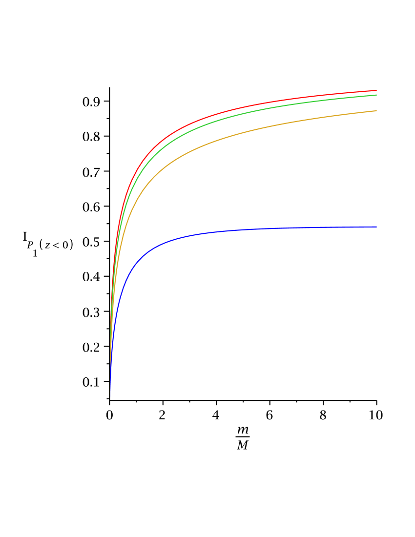
Figure 3: $I_{P^{(1)}_{1}(z<0)}$ versus mass ratio $m/M$ for different values of the coefficient of restitution $\alpha$: from top to bottom, $\alpha=0.99,0;8,0.5,0$.

For inelastic particles ($\alpha<1$), Fig. 3 shows that $I_{P^{(1)}_{1}(z<0)}$ increases with the mass ratio $m/M$ for all values of $\alpha$. For the sake of simplicity, $\gamma$ is assumed equal to $1$. Attention must be paid to the case $\alpha=0$: in this case, the limit of $I_{P^{(1)}_{1}(z<0)}$ when $m/M\rightarrow\infty$ is equal to $1/2$ whereas $I_{P^{(1)}_{1}(z<0)}$ goes to $1$ when $m/M\rightarrow\infty$ if $\alpha>0$. This discontinuity is clearly apparent in Fig.3.

III.2 Two dimensions

The first-collision velocity-correlation distribution can also be obtained analytically in two dimensions and above. Indeed the calculation can be performed following a method used in the one-dimensional case. Let us note that the scalar product of the pre- and post-collisional velocities ${\bf v}.{\bf v}^{*}$ can be expressed in an orthonormal basis associated with the collision as

$${\bf v}.{\bf v^{*}} =v_{n}v_{n}^{*}+v_{t}v_{t}^{*},$$ (37)

where $v_{n}$ and $v_{t}$ denote the normal and tangential components of the velocity. The post-collisional quantities in the rhs of Eq.(37) can be eliminated by using Eq.(14):

$${\bf v}.{\bf v^{*}}=v_{t}^{2}+\frac{1-\alpha^{\prime}}{2}v_{n}^{2}+\frac{1+\alpha^{\prime}}{2}v_{n}u_{n},$$ (38)

where $u_{n}$ is the normal component of the velocity of the bath particle.

Since the normal and tangent components of the tracer particle are independent random variables, the integrals can be performed successively over $u_{n}$ and $v_{n}$ as in the one-dimensional case, provided that $z$ is shifted to $z-v_{t}^{2}$. It is worth noting that the last integration over angular variables (${\bf n}$) is trivial, since the integrand does not depend on ${\bf n}$.

For $z<0$, the decay of $P^{(2)}_{1}(z)$ remains exponential and is equal to

$$P^{(2)}_{1}(z)=P^{(1)}_{1}(0)\frac{e^{(ab+c)z}}{\sqrt{1+2(ab+c)\frac{\gamma T}{M}}}.$$ (39)

For $z>0$, $P^{(2)}_{1}(z)$ has two contributions,

$$P^{(2)}_{1}(z)=\frac{P^{(1)}_{1}(0)e^{(ab+c)z}}{\sqrt{1+2(ab+c)\frac{\gamma T}{M}}}erfc\left[\sqrt{z\left(\frac{M}{2\gamma T}+(ab+c)\right)}\right]$$

$$+P^{(1)}_{1}(0)\sqrt{\frac{M}{2\pi\gamma T}}e^{cz}\int_{0}^{z}dy\frac{1}{\sqrt{y}}e^{-(\frac{M}{2\gamma T}+c)y}$$

$$\left[e^{ab(z-y)}erfc\left[\frac{(a+b)\sqrt{(z-y)}}{\sqrt{2}}\right]\right.$$

$$\left.+\frac{a-b}{a+b}e^{-ab(z-y)}erf\left[\frac{(a-b)\sqrt{(z-y)}}{\sqrt{2}}\right]\right].$$ (40)

Note that $P^{(2)}_{1}(z)$ has an exponential decay when the scalar product of velocities is negative (i.e. $z<0$), with the same coefficient $(ab+c)$ than we have obtained in one dimension. The integration over $v_{t}$ only changes the normalization constant compared to the one-dimensional case. Conversely, for positive arguments $z$, the shape of $P^{(2)}_{1}(z)$ is more complicated than in one dimension. As will be seen in the next section, the exponential decay of $P^{(2)}_{1}(z)$ is universal since this result is the same in any dimension and for different heating mechanisms (through the $\gamma$ dependence). The fraction of events in which the scalar product between the pre and post-collisional velocities is negative is then given by

$$I_{P^{(2)}_{1}(z<0)}=\frac{(a+b)(ab-c)}{2ab\sqrt{a^{2}+b^{2}-2c}}\frac{1}{\sqrt{1+2(ab+c)\frac{\gamma T}{M}}},$$ (41)

where $a$, $b$ and $c$ are given by Eqs.(21)-(23).

For instance, for elastic hard particles, the fraction of events in which the scalar product is negative after a collision is given by

$$I_{P^{(2)}_{1}(z<0)}=\sqrt{\frac{m}{m+M}}\sqrt{\frac{m}{M+2m}}.$$ (42)

Therefore, for a monodisperse system ($m=M$), $I_{P^{(2)}_{1}(z<0)}=1/\sqrt{6}\simeq 0.40824..$ in $2D$ whereas $I_{P^{(1)}_{1}(z<0)}=1/\sqrt{2}\simeq 0.707..$ in $1D$. In other words, in $2D$, most collisions do not change the scalar product, whereas the converse is observed in $1D$.

III.3 Three dimensions

In three dimensions, the first-collision velocity-correlation distribution can be similarly derived. The scalar product between the pre- and post-collisional velocities can be expressed as

$${\bf v}.{\bf v^{*}} =v_{n}v_{n}^{*}+v_{t}v_{t}^{*}+v_{z}v_{z}^{*}$$

$$=\frac{1-\alpha^{\prime}}{2}v_{n}^{2}+\frac{1+\alpha^{\prime}}{2}v_{n}u_{n}+v_{t}^{2}+v_{z}^{2},$$ (43)

where $u_{n}$ is the normal component of the velocity of the bath particle. $P^{(3)}_{1}(z)$ is the probability distributions associated with the sum of two independent random variables. The first one is the 1D collision term $\frac{1-\alpha^{\prime}}{2}v_{n}^{2}+\frac{1+\alpha^{\prime}}{2}v_{n}u_{n}$ and the second one is the sum $v_{1t}^{2}+v_{1z}^{2}$, which is a $\chi^{2}_{2}$-distributed variable, and, as a result, an exponentially distributed variable :

$$\chi^{2}_{2}(y)=\frac{M}{2\gamma T}e^{-\frac{My}{2\gamma T}}.$$ (44)

$P^{(3)}_{1}(z)$ can be expressed as the convolution product of the two probability distributions of these variables. As the distributions are normalized, the distribution obtained via the convolution product is normalized. For $z<0$,

$$P^{(3)}_{1}(z)= P^{(1)}_{1}(0)\frac{M}{2\gamma T}\int_{0}^{+\infty}dye^{-\frac{My}{2\gamma T}}e^{(ab+c)(z-y)}$$

$$= P^{(1)}_{1}(0)\frac{e^{(ab+c)z}}{1+2(ab+c)\frac{\gamma T}{M}}$$ (45)

and for $z>0$, $P^{(3)}_{1}(z)$ is the sum of several contributions :

$$P^{(3)}_{1}(z)=P^{(1)}_{1}(0)\left[\frac{M}{\gamma T}\frac{e^{(ab+c)z}erfc\left[\frac{(a+b)\sqrt{z}}{\sqrt{2}}\right]}{\frac{M}{\gamma T}+2(ab+c)}\right.$$

$$+\frac{M}{\gamma T}\frac{(b-a)e^{(-ab+c)z}erf\left[\frac{(a-b)\sqrt{z}}{\sqrt{2}}\right]}{(a+b)(-\frac{M}{\gamma T}+2ab-2c)}$$

$$\left.+\frac{M}{\gamma T}\frac{4abe^{-\frac{Mz}{2\gamma T}}\sqrt{a^{2}+b^{2}-2c-\frac{M}{\gamma T}}erf\left[\frac{\sqrt{z}\sqrt{a^{2}+b^{2}-2c-\frac{M}{\gamma T}}}{\sqrt{2}}\right]}{(a+b)(-\frac{M}{\gamma T}+2ab-2c)(\frac{M}{\gamma T}+2(ab+c))}\right],$$ (46)

where $a$, $b$, and $c$ are given by Eq.(21)-(23) and $\gamma$ is the temperature ratio.

As already noted, $P^{(3)}_{1}(z)$ has the same $z$ dependence as in 1D and 2D when $z<0$. The influence of the dimension is in the amplitude factor which decreases when the dimension increases, the temperature and other microscopic parameters (masses, coefficient of restitution) being kept constant.

From Eq.(45), the fraction of events with a negative velocities scalar product can be exactly obtained; moreover, a general formula can be obtained in any dimension:

$$I_{P^{(d)}_{1}(z<0)}=\frac{(a+b)(ab-c)}{2ab\sqrt{a^{2}+b^{2}-2c}}\left(1+2(ab+c)\frac{\gamma T}{M}\right)^{\frac{1-d}{2}}.$$ (47)

IV Influence of the Sonine corrections of the velocity distribution on $P^{(1)}_{1}(z)$

For granular gases, whose kinetic properties are well described by the Boltzmann equation, the velocity distribution is no longer a Gaussian. The deviations from Gaussian behavior can be captured by Sonine corrections. It is then possible to quantify the influence of these corrections on the distribution $P_{1}(z)$. (since the definition of the latter does not depend on the details of the velocity distribution function).

The non-linear Boltzmann equation can be solved numerically by using a Direct Simulation Monte Carlo (DSMC) methodB94 ; MS00 . We have performed DSMC simulations for monodisperse homogeneous systems excited through a stochastic thermostat. This allowed us to compare the distribution $P_{1}(z)$ obtained by simulation with the theoretical prediction calculated with a Sonine correction.

The calculation is similar to that of Eq.(III.1), but in the case studied here we no longer consider a tracer particle, so that $f=f_{B}$. Calculations were performed by considering only the first correction. This gives :

$$f({\bf v})=\left(\frac{M}{2\pi T}\right)^{d/2}e^{-\frac{M{\bf v}^{2}}{2T}}\left(1+a_{2}(\alpha)S_{2}\left(\frac{M{\bf v}^{2}}{2T}\right)\right),$$ (48)

where $S_{2}$ is the second Sonine polynomial expressed in the appropriate dimension. The value of $a_{2}(\alpha)$ is taken equal to its usual approximation for the stochastic thermostatVE98 ; MS00 . As the form of the perturbation introduced is simply a multiplicative polynomial, the expressions obtained for the 1D distribution $P^{(1)}_{1}(z)$ are analytical. As the result for $z>0$ is involved, we will only provide that obtained for $z<0$, which is

$$P^{(1)}_{1}(z)=\frac{e^{\frac{Mz}{T}\frac{2\left(1-\alpha+\sqrt{2}\sqrt{1+\alpha^{2}}\right)}{(1+\alpha)^{2}}}}{64\sqrt{2\pi}\left(1+\alpha+\alpha^{2}+\alpha^{3}\right)^{3}}\times$$

$$\times\left(Q(\alpha)+a_{2}(\alpha)\left(Q_{0}(\alpha)+\frac{Mz}{T}Q_{1}(\alpha)+\frac{M^{2}z^{2}}{T^{2}}Q_{2}(\alpha)\right)\right)$$ (49)

where the $Q_{i}(\alpha)$’s are simple functions of $\alpha$ given in Appendix B.

Since the 2D case is closer to possible experimental systems, we have also included Sonine corrections to the velocity distribution for calculating the velocity-correlation distribution $P^{(2)}_{1}(z)$, but the lengthy expressions are not given here. Figure 4 displays the analytical result ($P^{(2)}_{1}(z)$ with Sonine corrections) and the DSMC results for two values of the coefficient of restitution : $\alpha=0.2,0.5$. Even for the more inelastic case, the agreement between analytical results and DSMC is remarkable.

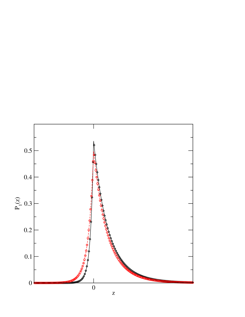
Figure 4: DSMC results(symbols) and theoretical predictions with the first Sonine correction(lines) for $P^{(2)}_{1}(z)$ versus $z=mv_{1}v^{\prime}_{1}/T$ in 2D. Diamonds and circles correspond respectively to the simulations for $\alpha=0.2,0.5$, respectively.

V Second and higher-collision velocity-correlation distributions

The collision statistics can be followed beyond the first-collision distribution. Formally, the second-collision velocity-correlation distribution $P_{2}(z)$ is given by the relation

$$P_{2}(z) =C_{2}\int_{S_{1}}\int_{S_{2}}\int\int d{\bf n}_{1}d{\bf n}_{2}d{\bf u}_{1}d{\bf u}_{2}d{\bf v}|({\bf u}_{1}-{\bf v}_{1}).{\bf n}_{1}|$$

$$|({\bf u}_{2}-{\bf v}_{1}^{*}).{\bf n}|f({\bf v})f_{B}({\bf u}_{1})f_{B}({\bf u}_{2})\delta(z-{\bf v}.{\bf v}_{2}^{*}),$$ (50)

where ${\bf v}_{1}$ denotes the pre-collisional velocity of the tagged particle for the first collision, ${\bf v}_{1}^{*}$ the velocity after the first collision and ${\bf v}_{2}^{*}$ the post-collisional velocity after the second collision. ${\bf u}_{1}$ and ${\bf u}_{2}$ correspond to the velocities of the bath particles for the first and second collisions, respectively. (Recall that $f({\bf v})$ and $f_{B}({\bf v})$ are the velocity distributions of the tagged and bath particles, respectively). Obviously, ${\bf v}_{2}={\bf v}_{1}^{*}$, and by using Eq.(14), the collision rule gives for the two collisions

$${\bf v}_{1}^{*} ={\bf v}_{1}+\frac{1+\alpha^{\prime}}{2}[({\bf u}_{1}-{\bf v}_{1}).{\bf n}_{1}]{\bf n}_{1},$$ (51)

$${\bf v}_{2}^{*} ={\bf v}_{1}^{*}+\frac{1+\alpha^{\prime}}{2}[({\bf u}_{2}-{\bf v}_{2}).{\bf n}_{2}]{\bf n}_{2}.$$ (52)

Finally, $C_{2}$ is the normalization constant ensuring that

$$\int_{-\infty}^{\infty}dzP^{(1)}_{2}(z)=1.$$ (53)

In a similar way, it is possible to write down closed equations for $P_{n}(z)$. However, whereas tractable expressions have been obtained in any dimension for $P_{1}(z)$, the calculation increases drastically in complexity for obtaining the distribution at the second collision. In the restricted case where $\alpha^{\prime}=1$ in one dimension, it is nonetheless possible to obtain the exact expression of $P^{(1)}_{2}(z)$ (details of the calulation are given in Appendix C). Thus, for $z<0$,

$$P^{(1)}_{2}(z) =C^{\prime}_{2}\left(\left(\frac{e^{\sqrt{2}abz}}{a}+\frac{e^{b\sqrt{a^{2}+b^{2}}z}}{b}\right)+\frac{(1+b^{2}z)}{b}\times\right.$$

$$\left.\times\int_{0}^{\infty}dv\frac{e^{-\frac{a^{2}v^{2}}{2}-\frac{b^{2}z^{2}}{2v^{2}}}}{v}\left[erfc\left(\frac{bv}{\sqrt{2}}\right)+erf\left(\frac{bz}{\sqrt{2}v}\right)\right]\right)$$ (54)

and for $z>0$,

$$P^{(1)}_{2}(z) =C^{\prime}_{2}\left(\frac{\sqrt{2\pi}}{b^{2}}\left(\frac{e^{-\sqrt{2}abz}}{a}erf\left(\frac{(\sqrt{2}a-2b)\sqrt{z}}{2}\right)\right.\right.$$

$$+\frac{e^{\sqrt{2}abz}}{a}erfc\left(\frac{(\sqrt{2}a+2b)\sqrt{z}}{2}\right)$$

$$-\frac{e^{-b\sqrt{a^{2}+b^{2}}z}}{b}erfc\left(\frac{(-b+\sqrt{a^{2}+b^{2}})\sqrt{z}}{\sqrt{2}}\right)$$

$$+\frac{e^{b\sqrt{a^{2}+b^{2}}z}}{b}erfc\left(\frac{(b+\sqrt{a^{2}+b^{2}})\sqrt{z}}{\sqrt{2}}\right)$$

$$+2\frac{\sqrt{2\pi}(1+b^{2}z)}{b^{3}}\int_{\sqrt{z}}^{\infty}dv\frac{e^{-\frac{a^{2}v^{2}}{2}-\frac{b^{2}z^{2}}{2v^{2}}}}{v}\times$$

$$\left.\left[erfc\left(\frac{bv}{\sqrt{2}}\right)+erf\left(\frac{bz}{\sqrt{2}v}\right)\right]\right),$$ (55)

where $C^{\prime}_{2}$ is determined from Eq. (53) and, with the help of Eqs.(21) and (22), $a=\sqrt{\frac{M}{\gamma T}}$ and $b=\sqrt{\frac{m}{T}}$. From Eqs.(V) and (V), one obtains the small-$z$ expansion for $P^{(1)}_{2}(z)$ :

$$P^{(1)}_{2}(z)\sim K_{0}(\sqrt{\frac{ab}{\gamma}}\frac{|z|}{T}).$$ (56)

Therefore, the second-collision velocity-correlation distribution shows a divergence at $z=0$, reminiscent of the divergence of $P^{(1)}_{\infty}(z)$, when the two velocities are completely uncorrelated. However, note that the coefficient of the modified Bessel function of the second kind $K_{0}(z)$ is $ab$ instead of $a^{2}$ for $P^{(1)}_{\infty}(z)$. To continue the analysis of the velocity-correlation distributions in general, we have performed DSMC in various situations, and monitored several $P^{(1)}_{n}(z)$’s.

Figure 5 shows $P^{(1)}_{n}(z)$ as a function of $z$ for $n=1,2..10$. Note that for $n\geq 3$, the distribution practically reaches the asymptotic value, namely $P_{\infty}(z)$. A simple physical interpretation is that after $3$ collisions the systems loses memory of its initial velocity configuration, and the correlation between the initial velocity and the velocity after $n$ collisions vanishes when $n$ is larger than $3$. Similar plots are displayed in Figs. 6 and 7 for $P^{(2)}_{n}(z)$ and $P^{(3)}_{n}(z)$, respectively. One notes that the convergence to the asymptotic function, $P_{\infty}(z)$, becomes slower when the space dimension increases.

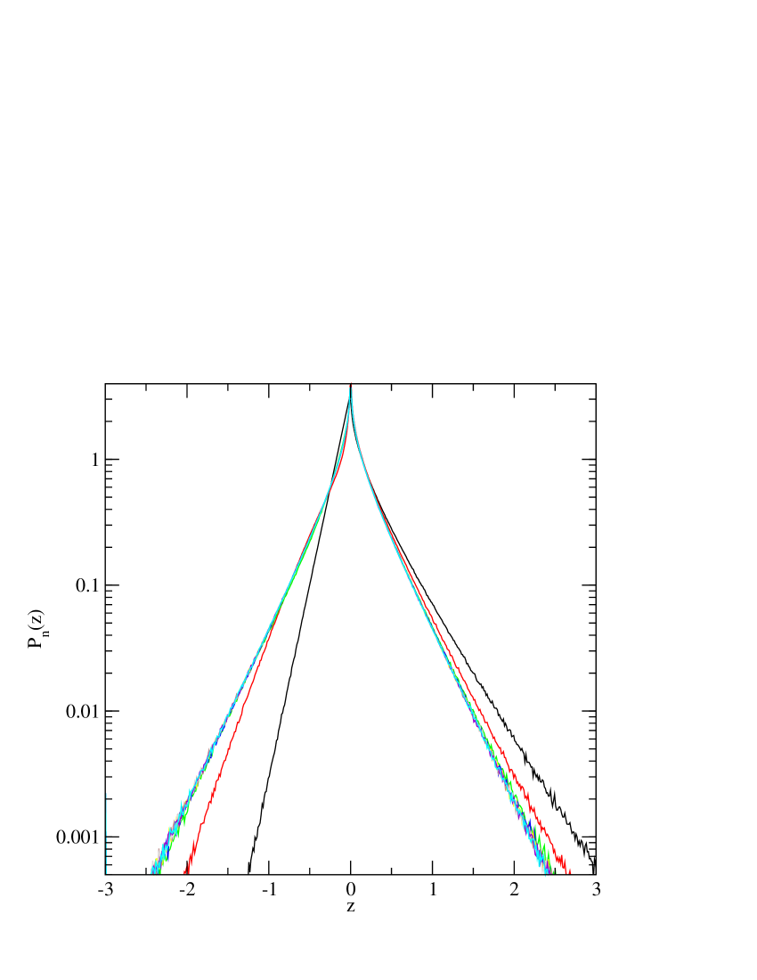
Figure 5: $nth$ collision velocity-correlation distributions $P^{(1)}_{n}(z)$ versus $z$ for various values of $n$: $n=1,2,..10$ ($D=1$).

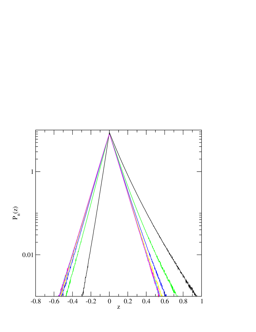
Figure 6: $nth$ collision velocity-correlation distributions $P^{(2)}_{n}(z)$ versus $z$ for various values of $n$: $n=1,2,..,10$ ($D=2$).

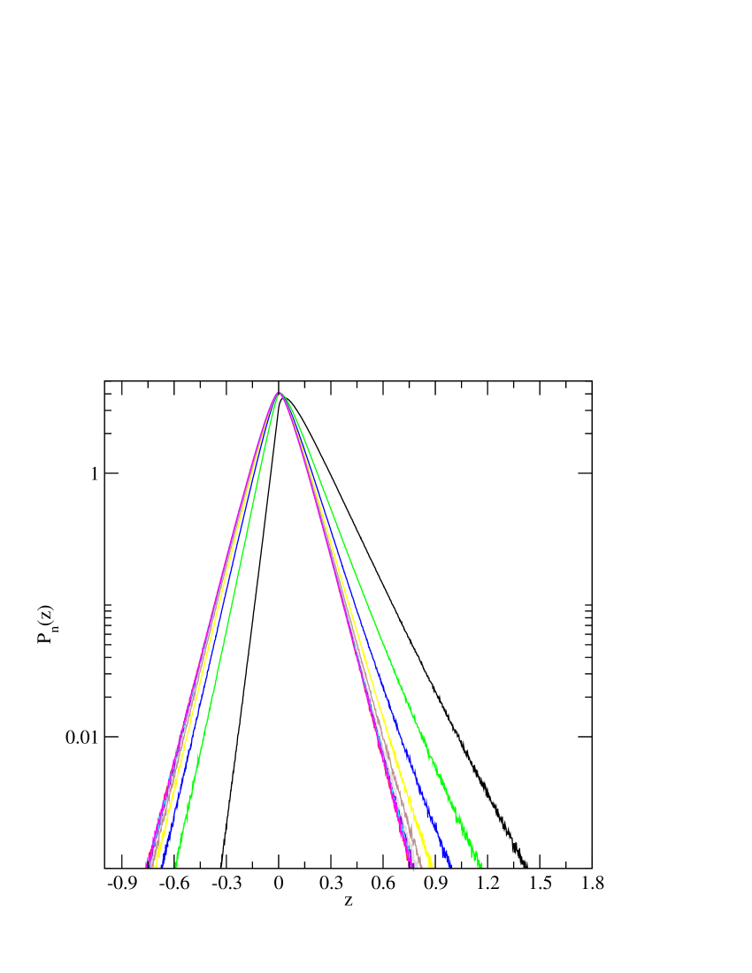
Figure 7: $nth$ collision velocity-correlation distributions $P^{(3)}_{n}(z)$ versus $z$ for various values of $n$: $n=1,2,..,10$ ($D=3$).

VI Conclusion

We have introduced new velocity-correlation distributions that capture the early stages of the dynamics. These non-trivial quantities are efficient probes for investigating the environment of a particle in granular gases. We have shown that these distributions decay exponentially when the scalar product of the velocities is negative.

Other interesting physical situations could be considered: free cooling states, in which the velocity distribution obeys a scaling form, binary mixturesBT02 ; BMP02 ; S03 , and not only in the infinite dilution limit considered in this paper.

These distributions are easily accessible in computer simulations, and probably, in experiments; indeed, when the time resolution is smaller than the mean collision time, the probability that two collisions occur during a time step is small and the collision history can be monitored accurately, which permits to build the first-collision velocity-correlation distributions.

VII Acknowledgments

We thank Kristin Combs, Jeffrey Olafsen, Julian Talbot and Gilles Tarjus for suggestions and fruitful discussions.

Appendix A 1D first-collisions

We have the following integrals, for $z<0$,

$$\int_{0}^{+\infty}dv(1-\frac{z}{v^{2}})\exp\left(-\frac{a^{2}v^{2}}{2}-\frac{b^{2}z^{2}}{2v^{2}}\right)=\frac{a+b}{ab}\sqrt{\frac{\pi}{2}}e^{abz}$$ (57)

and for $z>0$,

$$\int_{0}^{\sqrt{z}}dv(\frac{z}{v^{2}}-1)\exp\left(-\frac{a^{2}v^{2}}{2}-\frac{b^{2}z^{2}}{2v^{2}}\right)=$$

$$\sqrt{\frac{\pi}{2}}\frac{1}{2ab}\left((a-b)e^{-abz}\left(erf\left(\frac{a-b}{\sqrt{2}}\sqrt{z}\right)+1\right)+\right.$$

$$\left.(a+b)e^{abz}erfc\left(\frac{a+b}{\sqrt{2}}\sqrt{z}\right)\right)$$ (58)

and

$$\int_{\sqrt{z}}^{\infty}dv(1-\frac{z}{v^{2}})\exp\left(\frac{a^{2}v^{2}}{2}-\frac{b^{2}z^{2}}{2v^{2}}\right)=$$

$$\sqrt{\frac{\pi}{2}}\frac{1}{2ab}\left((a-b)e^{-abz}\left(erf\left(\frac{a-b}{\sqrt{2}}\sqrt{z}\right)-1\right)+\right.$$

$$\left.(a+b)e^{abz}erfc\left(\frac{a+b}{\sqrt{2}}\sqrt{z}\right)\right),$$ (59)

which gives for $z<0$

$$P^{(1)}_{1}(z)=\frac{4C}{(1+\alpha^{\prime})^{2}}\frac{a+b}{ab}e^{(ab+c)z}$$ (60)

and for $z>0$

$$P^{(1)}_{1}(z) =\frac{4C}{(1+\alpha^{\prime})^{2}}\sqrt{\frac{\pi}{2}}e^{cz}\left(\frac{a-b}{ab}e^{-abz}\left(erf\left(\frac{a-b}{\sqrt{2}}\sqrt{z}\right)\right)\right.+$$

$$+\left.\frac{a+b}{ab}e^{abz}erfc\left(\frac{a+b}{\sqrt{2}}\sqrt{z}\right)\right).$$ (61)

The constant $C$ can be obtained by calculating the normalization condition $\int dzP_{1}(z)=1$, which gives

$$C=\frac{(1+\alpha^{\prime})^{2}}{4}\frac{a^{2}b^{2}-c^{2}}{\sqrt{2\pi(a^{2}+b^{2}-2c)}}.$$ (62)

Appendix B Sonine correction to the 1D calculation

For $z<0$, one finds

$$P^{(1)}_{1}(z)=e^{\frac{2(1-\alpha)}{(1+\alpha)^{2}}\frac{Mz}{T}}C\int_{0}^{\infty}du(1-\frac{z}{u^{2}})$$

$$\exp\left(-\frac{M}{T}\left(\frac{(1+\alpha^{2})u^{2}}{(1+\alpha)^{2}}+\frac{2z^{2}}{u^{2}(1+\alpha)^{2}}\right)\right)$$

$$\left(1+a_{2}(\alpha)\left(S_{2}\left(\frac{Mu^{2}}{2T}\right)+S_{2}\left(\frac{Mu^{2}}{T}\frac{(2z/u^{2}-(1-\alpha))^{2}}{2(1+\alpha)^{2}}\right)\right)\right).$$ (63)

After integration of Eq.(B), one obtains

$$P^{(1)}_{1}(z) =\frac{P_{1}(0)}{Q(\alpha)+a_{2}(\alpha)Q_{0}(\alpha)}e^{\frac{Mz}{T}\frac{2\left(1-\alpha+\sqrt{2}\sqrt{1+\alpha^{2}}\right)}{(1+\alpha)^{2}}}$$

$$\left(Q(\alpha)+a_{2}(\alpha)\left(Q_{0}(\alpha)+\frac{Mz}{T}Q_{1}(\alpha)+\frac{M^{2}z^{2}}{T^{2}}Q_{2}(\alpha)\right)\right)$$ (64)

where

$$Q(\alpha)= 16(1+\alpha)^{4}\left(1+\alpha^{2}\right)^{2}$$

$$\left(1+\alpha^{2}+\sqrt{2}\sqrt{1+\alpha^{2}}\right),$$ (65)

$$Q_{0}(\alpha) =3(1+\alpha)^{4}$$

$$\left(2+6\alpha^{2}+6\alpha^{4}+2\alpha^{6}+\sqrt{2}\sqrt{1+\alpha^{2}}\left(1+6\alpha^{2}+\alpha^{4}\right)\right),$$ (66)

$$Q_{1}(\alpha)=2\sqrt{2}(1+\alpha)^{2}\left(1+\alpha^{2}\right)^{3/2}$$

$$(37-12\alpha+42\alpha^{2}-20\alpha^{3}+17\alpha^{4})$$

$$+2(1+\alpha)^{2}\left(1+\alpha^{2}\right)(54-16\alpha$$

$$+84\alpha^{2}-32\alpha^{3}+54\alpha^{4}-16\alpha^{5}),$$ (67)

$$Q_{2}(\alpha)=8\left(1+\alpha^{2}\right)(3-2\alpha+3\alpha^{2})$$

$$\left((7-6\alpha+3\alpha^{2})\left(1+\alpha^{2}\right)+\sqrt{2}\sqrt{1+\alpha^{2}}\right.$$

$$\left.\left(5-4\alpha+5\alpha^{2}-2\alpha^{3}\right)\right).$$ (68)

Appendix C Second-collision velocity-correlation distribution

In one dimension when $\alpha^{\prime}=1$, the velocities of the tagged particle and the bath particle are exchanged during the collision. This drastically simplifies the expression of the second-collision velocity-collision distribution and the calculation becomes tractable. Indeed, if $\alpha^{\prime}=1$, $P^{(1)}_{2}(z)$ becomes

$$P^{(1)}_{2}(z)=C_{2} \int dv\int du_{1}\int du_{2}|u_{1}-v||u_{2}-u_{1}|f_{B}(u_{1})\times$$

$$\times f_{B}(u_{2})f(v)\delta(vu_{2}-z),$$ (69)

where $f_{B}(u)$ denotes the bath velocity distribution and $f(v)$ the tagged particle velocity distribution.

We first integrate on the velocity of the bath particle $2$, namely the velocity of the colliding particle at the second collision. We drop the subscript of the velocity of the bath particle for the collision $1$, and $P^{(1)}_{2}(z)$ reads

$$P^{(1)}_{2}(z)=C_{2}\int dv\int du|u-v||\frac{z}{v^{2}}-u|f_{B}(u)f_{B}\left(\frac{z}{v^{2}}\right)f(v).$$ (70)

Let us introduce the function $I(z,v)$ :

$$I(z,v)=\int du|u-v||z-uv|e^{-\frac{b^{2}u^{2}}{2}}.$$ (71)

When $z<v^{2}$, one has

$$I(z,v) =\frac{2v^{2}}{b^{2}}e^{-\frac{b^{2}z^{2}}{2v^{2}}}-\frac{2z}{b^{2}}e^{-\frac{b^{2}v^{2}}{2}}+\frac{\sqrt{2\pi}|v|(1+b^{2}z)}{b^{3}}$$

$$+\frac{\sqrt{2\pi}v(1+b^{2}z)}{b^{3}}\left(erf\left(\frac{bz}{\sqrt{2v}}\right)-erf\left(\frac{bv}{\sqrt{2}}\right)\right).$$ (72)

and when $z>v^{2}$

$$I(z,v) =-\frac{2v^{2}}{b^{2}}e^{-\frac{b^{2}z^{2}}{2v^{2}}}+\frac{2z}{b^{2}}e^{-\frac{b^{2}v^{2}}{2}}-\frac{\sqrt{2\pi}|v|(1+b^{2}z)}{b^{3}}$$

$$-\frac{\sqrt{2\pi}v(1+b^{2}z)}{b^{3}}\left(erf\left(\frac{bz}{\sqrt{2v}}\right)-erf\left(\frac{bv}{\sqrt{2}}\right)\right)$$ (73)

Inserting Eq.(C) in Eq. (C) and integrating out the first two terms of the integrand leads to Eq.(V). For $z>0$, by using the property of $I(v,z)$ (Eqs.(C)- (C)), for $z>0$, $P_{2}(z)$ is expressed as

$$P^{(1)}_{2}(z)=C_{2}\left(\int_{\sqrt{z}}^{\infty}dv-\int^{\sqrt{z}}_{0}dv\left(\frac{e^{-\frac{a^{2}v^{2}}{2}-\frac{b^{2}z^{2}}{2v^{2}}}}{v^{2}}I(v,z)\right)\right).$$ (74)

Integrating out the first terms of the right-hand-side of Eq.(74) leads to Eq.(V).

References

- (1) N. V. Brilliantov and T. Pöschel, Kinetic theory of granular gases (Oxford University Press, Oxford, 2004).
- (2) G. W. Baxter and J. S. Olafsen, Phys. Rev. Lett. 99, 028001 (2007).
- (3) P. Visco, F. vanWijland, and E. Trizac, J. Phys. Chem. B 112, 5412 (2008).
- (4) P. Visco, F. van Wijland, and E. Trizac, Phys. Rev. E 77, 041117 (2008).
- (5) J. Talbot, Molecular Physics 75, 43 (1992).
- (6) L. Lue, J. Chem. Phys. 122, 044513 (2005).
- (7) A. Puglisi, P. Visco, E. Trizac, and F. van Wijland, Phys. Rev. E 73, 021301 (2006).
- (8) A. Santos and J. W. Dufty, Phys. Rev. Lett. 97, 058001 (2006).
- (9) J. Piasecki, J. Talbot, and P. Viot, Physica A 373, 313 (2006).
- (10) P. A. Martin and J. Piasecki, Europhys. Lett. 46, 613 (1999).
- (11) V. Garzó and J. Dufty, Phys Rev E 60, 5706 (1999).
- (12) J. J. Brey, M. J. Ruiz-Montero, and F. Moreno, Physical Review Letters 95, 098001 (2005).
- (13) G. Bird, Molecular gas dynamics and the direct simulation of gas flows (Clarendon Press, Oxford, England, 1994).
- (14) J. M. Montanero and A. Santos, Granular Matter 2, 53 (2000).
- (15) T. P. C. van Noije and M. H. Ernst, Granular Matter 1, 57 (1998).
- (16) A. Barrat and E. Trizac, Granular Matter 4, 57 (2002).
- (17) T. Biben, P. A. Martin, and J. Piasecki, Physica A 310, 308 (2002).
- (18) A. Santos, Phys. Rev. E 67, 051101 (2003).