Quantum Ratchet Accelerator without a Bichromatic Lattice Potential

Abstract

In a quantum ratchet accelerator system, a linearly increasing directed current can be dynamically generated without using a biased field. Generic quantum ratchet acceleration with full classical chaos [Gong and Brumer, Phys. Rev. Lett. 97, 240602 (2006)] constitutes a new element of quantum chaos and an interesting violation of a sum rule of classical ratchet transport. Here we propose a simple quantum ratchet accelerator model that can also generate linearly increasing quantum current with full classical chaos. This new model does not require a bichromatic lattice potential. It is based on a variant of an on-resonance kicked-rotor system, periodically kicked by two optical lattice potentials of the same lattice constant, but with unequal amplitudes and a fixed phase shift between them. The dependence of the ratchet current acceleration rate on the system parameters is studied in detail. The cold-atom version of our new quantum ratchet accelerator model should be realizable by introducing slight modifications to current cold-atom experiments.

I introduction

A ratchet accelerator (RA) Gongpre04 can generate, without using a biased field, directed transport in both the momentum and coordinate space. Specifically, certain spatio-temporal symmetries in the Hamiltonian dynamics are broken and as a result a linearly increasing directed current can be dynamically generated. Such a property of RA systems is of considerable interest for understanding (i) general properties of quantum and classical ratchet effects in Hamiltonian systems Gongpre04 ; schanzprl ; tania ; cheon ; schanzpre ; ratchetreview ; denisov ; lundh ; kenfack , (ii) quantum-classical correspondence in transport phenomena schanzprl ; tania ; schanzpre , and (iii) a number of interesting topics in quantum chaos casatibook .

Ongoing cold-atom studies of the well-known quantum kicked-rotor (QKR) model casatibook have motivated several RA studies using QKR variants. In particular, Ref. lundh showed that accelerating quantum ratchet current can be realized by considering a QKR variant, with the kicking period on the main resonance with the recoil frequency of the cold atoms. Reference kenfack showed that a quantum RA can also be realized with QKR variants on high-order quantum resonances. In both cases, spatio-temporal symmetries in the dynamics are broken by using a bichromatic optical lattice (specifically, an optical super-lattice obtained by superimposing two stand-waves with periods $\lambda/2$ and $\lambda/4$). However, though already achieved in some static cases weitz , experimentally realizing bichromatic and pulsed optical lattices is somewhat demanding. Indeed, in two recent cold-atom on-resonance-QKR experiments sadgrove ; danaprl , directed quantum transport is effectively demonstrated by use of a single-period optical lattice only, with the price being that special symmetry-breaking initial superposition states should be prepared.

The ratchet transport in the above-mentioned on-resonance-QKR models lundh ; sadgrove ; danaprl ; kenfack ; baowen occurs only for isolated values of the effective Planck constant (to be defined below). By contrast, using variants of another paradigm of quantum chaos, namely, the kicked-Harper model KHM , Gong and Brumer Gongprl06 proposed a quantum RA model that works for an arbitrary value of the effective Planck constant. In this sense, the ratchet transport in this new model Gongprl06 is generic. Furthermore, this generic RA model works even when the underlying classical dynamics is fully chaotic, a situation where classical ratchet transport necessarily vanishes according to a classical “sum rule” schanzpre ; schanzprl . Hence the work in Ref. Gongprl06 represents an interesting and generic quantum violation of a classical theorem.

The detailed aspects of the above-mentioned quantum violation of the classical sum rule are yet to be explored. Along this direction, a cold-atom realization of a generic quantum RA model would be of great interest. Nevertheless, such experiments were thought to be challenging because the model proposed in Ref. Gongprl06 also employed a flashing bichromatic optical lattice and it was unclear how a kicked-Harper-like model can be realized in a cold-atom laboratory.

Thanks to our recent finding jiaopra08 ; jiaojmo that exposed a direct connection between QKR and a class of kicked-Harper-like models, here we are able to propose a quantum RA model that (i) contains all the important ingredients as the model proposed in Ref. Gongprl06 , (ii) does not require a bichromatic lattice potential, and (iii) is realizable by slightly modifying existing cold-atom experiments of QKR dynamics. Indeed, this new RA model only requires an on-resonance variant of QKR, kicked by two optical lattice potentials of the same lattice constant, but with unequal kicking amplitudes and a fixed phase shift between them. In addition to offering a simpler quantum RA model that is of theoretical interest, it is hoped that our results below will motivate cold-atom experimental studies in the near future.

This paper is organized as follows. In Sec. II we show how a wide class of twisted kicked Harper models can be realized by using an on-resonance “double-kicked” rotor model. General discussions in Sec. II directly lead to an atom-optics proposal for realizing the RA model proposed in Ref. Gongprl06 . In Sec. III we simplify the cold-atom RA realization in Sec. II, resulting in a new RA model that does not need a bichromatic optical lattice potential. We then present and discuss detailed numerical results of our new RA model, with an emphasis placed on the dependence of the current acceleration rate on the system parameters. In Sec. IV we briefly discuss one extension of this study. Section V concludes this work.

II Cold-Atom Realizations of A Wide Class of Twisted Kicked Harper Models

Our starting point is the so-called double kicked-rotor model (DKRM) DKR1 ; DKR2 ; DKR3 that has been experimentally realized. We use scaled and dimensionless variables throughout. The DKRM Hamiltonian is then given by

$$H_{\text{DKRM}} = \frac{p^{2}}{2}+KV_{K}(q)\sum_{n}\delta(t-nT)$$ (1)

$$+ LV_{L}(q)\sum_{n}\delta(t-nT-\eta),$$

where $q$ ($\in[0,2\pi)$) and $p$ are conjugate coordinate and momentum operators, $T$ is the period for both kicking sequences, $\eta$ is the time delay between the two kicking sequences, $K$ and $L$ characterize the amplitudes of the kicking fields, $V_{K}(q)$ and $V_{L}(q)$ are periodic functions of $q$ with the period $2\pi$. The associated quantum map $U_{\text{DKRM}}$ for a period from $nT+0^{-}$ to $(n+1)T+{0}^{-}$ is given by

$$U_{\text{DKRM}}=e^{-i(T-\eta)\frac{p^{2}}{2\hbar}}e^{-i\frac{L}{\hbar}V_{L}(q)}e^{-i\eta\frac{p^{2}}{2\hbar}}e^{-i\frac{K}{\hbar}V_{K}(q)},$$ (2)

where $\hbar$ represents an effective and dimensionless Planck constant for the DKRM system (hence $p=-i\hbar\partial/\partial q$).

Theoretically, we shall first focus on an ideal situation where cold atoms are injected with exactly zero quasi-momentum quasimom . With that simplification we may consider only a Hilbert space satisfying the periodic boundary condition associated with $q\rightarrow q+2\pi$. The quantum resonance condition $T\hbar=4\pi$ then leads to

$$e^{-iT\frac{p^{2}}{2\hbar}}=1,$$ (3)

reducing $U_{\text{DKRM}}$ to $U_{\text{DKRM}}^{\text{r}}$,

$${U}^{\text{r}}_{\text{DKRM}} = e^{i\eta\frac{p^{2}}{2\hbar}}e^{-i\frac{L}{\hbar}V_{L}(q)}e^{-i\eta\frac{p^{2}}{2\hbar}}e^{-i\frac{{K}}{\hbar}V_{K}(q)}$$ (4)

$$= e^{i\frac{\tilde{p}^{2}}{2\tilde{\hbar}}}e^{-i\frac{\tilde{L}}{\tilde{\hbar}}V_{L}(q)}e^{-i\frac{\tilde{p}^{2}}{2\tilde{\hbar}}}e^{-i\frac{\tilde{K}}{\tilde{\hbar}}V_{K}(q)},$$

where we have defined the rescaled momentum

$$\tilde{p}\equiv\eta p$$ (5)

and the rescaled kicking amplitudes

$$\tilde{K} \equiv \eta K,$$ (6)

$$\tilde{L} \equiv \eta L.$$ (7)

Due to the above momentum rescaling, the effective Planck constant now becomes

$$\tilde{\hbar}\equiv\eta\hbar.$$ (8)

Equations (6,7,8) show that the rescaled dimensionless system parameters $\tilde{K}$, $\tilde{L}$, and $\tilde{\hbar}$ can be easily tuned by adjusting the time delay between the two kicking sequences. Based on a previous DKRM experiment DKR1 , we estimate that in experiments the kicking amplitudes $\tilde{K}$ and $\tilde{L}$ can vary in the range of $0.1-100$, and the effective Planck constant $\tilde{\hbar}$ can at least vary in the range of $0.05-20$. Our computational studies in the next section will be based on these two ranges.

To gain insights into the quantum-resonance-reduced quantum map in Eq. (4), let us first re-interpreted it as follows. Reading the four factors in Eq. (4) from right to left, one sees that within each period $T$, in effect the system is first subject to one kick, followed by a free evolution of duration unity; then the system is kicked a second time, followed by a second free evolution of the same duration, but now with the free Hamiltonian given by

$$H_{\text{free}}=-\tilde{p}^{2}/2.$$ (9)

Such an effective Hamiltonian with a negative kinetic energy term was first considered in Ref. gongpre07 . With this interpretation, one may define an “$\eta$-classical” limit of this quantum map, i.e., the $\tilde{\hbar}\equiv\eta\hbar\rightarrow 0$ limit with fixed $\tilde{K}$ and $\tilde{L}$. This terminology is inspired by the so-called “$\epsilon$-classical” limit in early studies of QKR models in the presence of gravity Fishmancla . Let ${q}^{c}$ and $\tilde{p}^{c}$ be the counterparts of $q$ and $\tilde{p}$ in this “$\eta$-classical” limit, with their values right before $t=nT$ denoted by ${q}^{c}_{n}$ and $\tilde{p}^{c}_{n}$. Further defining

$${\cal P}^{c}\equiv{q}^{c}+\tilde{p}^{c},$$ (10)

one easily finds the classical map associated with the “$\eta$-classical” limit,

$${\cal P}_{n+1}^{c} = {\cal P}_{n}^{c}-\tilde{K}\frac{dV_{K}({q}^{c}_{n})}{d{q}^{c}_{n}}$$ (11)

$${q}^{c}_{n+1} = {q}^{c}_{n}+\tilde{L}\frac{dV_{L}({\cal P}^{c}_{n+1})}{d{\cal P}^{c}_{n+1}}.$$ (12)

In terms of the canonical pair $q^{c}$ and ${\cal P}^{c}$, the classical Hamiltonian $H^{\text{c}}_{\eta}$ that generates this “$\eta$-classical” map is then given by

$${H}^{\text{c}}_{\eta}=\tilde{L}V_{L}({\cal P}^{c})+\tilde{K}V_{K}(q^{c})\sum_{n}\delta(t-n).$$ (13)

Consider now the simplest choice for the kicking potentials, i.e., $V_{K}(q)=V_{L}(q)=\cos(q)$. Such a choice under the restriction $\tilde{K}=\tilde{L}$ was adopted by the original experiment DKR1 and previous theoretical studies of off-resonance DKRM DKR2 ; DKR3 . Substituting $V_{K}(q)=V_{L}(q)=\cos(q)$ into Eq. (13), the resulting “$\eta$-classical” Hamiltonian becomes precisely the classical kicked Harper model in terms of ${\cal P}^{c}$ and $q^{c}$ jiaopra08 . Returning to the old representation $(q^{c},\tilde{p}^{c})$, the obtained kicked Harper Hamiltonian becomes

$${H}^{\text{c}}_{\text{TKH}}=\tilde{L}\cos(\tilde{p}^{c}+q^{c})+\tilde{K}\cos(q^{c})\sum_{n}\delta(t-n).$$ (14)

Comparing the Hamiltonian ${H}^{\text{c}}_{\text{TKH}}$ with the standard kicked-Harper Hamiltonian as a function of $q^{c}$ and $\tilde{p}^{c}$, i.e.,

$${H}^{\text{c}}_{\text{KH}}=\tilde{L}\cos(\tilde{p}^{c})+\tilde{K}\cos(q^{c})\sum_{n}\delta(t-n),$$ (15)

we can regard ${H}^{\text{c}}_{\text{TKH}}$ as a “twisted” version of the standard kicked-Harper model ${H}^{\text{c}}_{\text{KH}}$. With this in mind, the quantum map in Eq. (4) in the case of $V_{K}(q)=V_{L}(q)=\cos(q)$ can be regarded as a quantized version of the twisted kicked Harper model.

We now apply this on-resonance DKRM strategy to realize a twisted version of the quantum RA model proposed in Ref. Gongprl06 . This RA model involves the classical Hamiltonian

$$H^{\text{c}}_{\text{BKH}} = \tilde{L}\cos(\tilde{p}^{c})$$

$$+\tilde{K}\left[\cos(q^{c}+\phi_{1})+\sin(2q^{c}+\phi_{2})\right]\sum_{n}\delta(t-n).$$

(16)

If we now consider the following scenario:

Scenario I:

$$V_{L}(q)=\cos(q);$$ (17)

$$V_{K}(q)=[\cos(q+\phi_{1})+\sin(2q+\phi_{2})],$$ (18)

then a twisted version of $H^{\text{c}}_{\text{BKH}}$ (i.e., in terms of ${\cal P}^{c}$ and $q^{c}$ rather than $\tilde{p}^{c}$ and $q^{c}$) naturally emerges from Eq. (13). Clearly then, at least for a twisted version, a cold-atom quantum version of the bichromatic generalized kicked Harper model $H^{\text{c}}_{\text{BKH}}$ is realizable, provided that a kicking bichromatic lattice potential such as $[\cos(q+\phi_{1})+\sin(2q+\phi_{2})]\sum_{n}\delta(t-n)$ can be realized. In the next section a simpler realization of quantum RA is obtained.

Before ending this section we make one important remark. In the standard kicked Harper model ${H}^{\text{c}}_{\text{KH}}$ in Eq. (15), the momentum variable is an abstract canonical variable. This becomes obvious if we consider the canonical equations of motion, yielding that the moving speed in the coordinate space is not proportional to the momentum. As such, it is unclear whether the momentum variable in the kicked Harper model can be directly related to the mechanical momentum of a moving particle. Dana managed to connect this abstract momentum variable with the mechanical momentum of a charged particle kicked by a special sequence of magnetic fields dana . Here, through the cold-atom realization of a wide class of twisted kicked Harper models, we are linking the momentum variable in the kicked Harper model with the mechanical momentum of cold atoms. Only through such connections can the expectation value of the momentum be interpreted as a current of moving particles.

III Ratchet Accelerator without a Bichromatic optical Lattice

Our discussions in the previous section make it clear that, in realizing a wide class of kicked-Harper-like models with on-resonance DKRM, the following canonical transformation or twist is necessarily involved:

$$(q^{c},\tilde{p}^{c})\rightarrow(q^{c},{\cal P}^{c}).$$ (19)

Due to this phase space twist, the resultant systems should assume different symmetry properties than those analyzed in terms of $q^{c}$ and ${\tilde{p}}^{c}$. Hence, the symmetry-breaking considerations in Ref. Gongprl06 no longer apply to twisted kicked-Harper-like models. As a result, the use of a bichromatic optical lattice as in Ref. Gongprl06 may not be the simplest approach for symmetry-breaking. It is this recognition that motivated us to seek a realization of a quantum RA without using a bichromatic lattice potential. This attempt is also consistent with a recent study of ratchet transport (in coordinate space only) using an off-resonance DKRM involving two optical lattices of the same lattice constant carlos .

Specifically, here we shall demonstrate that an on-resonance DKRM with the following alternative scenario,

Scenario II:

$$V_{K}(q)=\cos(q);$$ (20)

$$V_{L}(q)=\cos(q+\phi)$$ (21)

can already give rise to a simple quantum RA model if $K\neq L$. In addition to the on-resonance condition, this scenario only needs to introduce two small modifications to a previous DKRM experiment DKR1 . First, the two kicking sequences of optical lattice potentials should have different amplitudes. Second, there should be a fixed phase shift $\phi$ between these two optical lattice potentials.

Using Eq. (4), scenario II described above gives the following quantum map,

$${U}_{\text{RA}}=e^{i\frac{\tilde{p}^{2}}{2\tilde{\hbar}}}e^{-i\frac{\tilde{L}}{\tilde{\hbar}}\cos(q+\phi)}e^{-i\frac{\tilde{p}^{2}}{2\tilde{\hbar}}}e^{-i\frac{\tilde{K}}{\tilde{\hbar}}\cos(q)}.$$ (22)

Using Eq. (13), one then obtains the $\eta$-classical Hamiltonian of this quantum map,

$$H^{\text{c}}_{\text{RA}}=\tilde{L}\cos(q^{c}+\tilde{p}^{c}+\phi)+\tilde{K}\cos(q^{c})\sum_{n}\delta(t-n).$$ (23)

Let $|n\rangle$ be the eigenstates of the momentum operator $\tilde{p}$, with an eigenvalue $n\tilde{\hbar}$ for a Hilbert space with the periodic boundary condition. In the following we shall focus on the RA dynamics for the initial state $|0\rangle$. The classical analog of this initial state is a classical ensemble with $\tilde{p}^{c}=0$ and a random uniform distribution of $q^{c}$. Such an initial state is a trivial state because it is symmetric upon time-reversal operations or space-reflection operations. With this choice of the initial state, any induced current afterwards must be due to some broken spatio-temporal symmetries in the ensuing dynamics. It is also worth noting that the system described by Eq. (22) is invariant under the transformations $q\to 2\pi-q$, $\tilde{p}\to-\tilde{p}$ and $\phi\to-\phi$. As a result the current should undergo a sign change under $\phi\to-\phi$, leading to the expectation that the generation of a ratchet current is forbidden for $\phi=0$ or $\phi=\pi$. For this reason we focus on other values of $\phi$.

III.1 Examples of Accelerating Ratchet Current

Consider first a few computational examples depicted in Fig. 1. There, the time dependence of the quantum ratchet current, i.e., the expectation value of the scaled momentum, $\langle\tilde{p}\rangle$, is shown for some particular values of $\tilde{K}$, $\tilde{L}$, and $\phi$. The initial state is $|0\rangle$ and the time propagation due to the quantum map $U_{\text{RA}}$ is carried out by standard fast-Fourier-transformation techniques. The cases shown in Fig. 1 display spectacular linear acceleration of the ratchet current at a significant rate. In order to have a comparison with the underlying $\eta$-classical limit, we have also calculated the ensemble-averaged classical momentum, $\langle{\tilde{p}}^{c}\rangle$. The classical calculations are based on the $\eta$-classical map given by Eq. (23), using an ensemble of $10^{6}$ particles initially distributed along ${\tilde{p}}^{c}=0$ randomly and uniformly. As is seen from Fig. 1a, the $\eta$-classical currents can also increase linearly, with a slope smaller than their quantum counterparts. The result in Fig. 1b is even more interesting. There the classical current remains indistinguishable from zero at all times, but the quantum acceleration is substantial. Note also that these “$\eta$-classical” results have nothing to do with the true classical limit of a DKRM, because here the DKRM is always on the main quantum resonance. Indeed, the $\eta$-classical Hamiltonian is given by Eq. (23), whereas the true classical Hamiltonian of the DKRM should take exactly the same form as Eq. (1).

Figure 1: Time dependence of the ratchet current for both the quantum ratchet accelerator model of Eq. (22) (solid lines) and its $\eta$-classical limit (dash-dotted lines) described by Eq. (23). For panel (a), system parameters are $\tilde{\hbar}=1$, $\tilde{K}=3$, $\tilde{L}=1$, and $\phi=\pi/2$ (upper two curves), $\pi/3$ (bottom two curves). For panel (b), system parameters are $\tilde{\hbar}=1$, $\tilde{K}=4$, $\tilde{L}=2$, and $\phi=\pi/2$. The classical current in panel (b) remains indistinguishable from zero at all times because the system is in the full chaos regime (see Fig. 3d).

We have also checked that if we choose $\phi=0,\pi$ instead, then both the classical and quantum acceleration seen in the examples in Fig. 1a do vanish. This confirms our previous discussion on a symmetry property of our new RA model.

III.2 Dependence of Acceleration Rate on $\tilde{K}$ and $\tilde{L}$

To further explore the dynamical aspects of our new RA model, we have carried out detailed studies of how the ratchet acceleration rate depends on the system parameters. The computational examples shown in Fig. 1 motivate us to define the quantum current accelerate rate as follows:

$$R_{q}\equiv d\langle\tilde{p}(t)\rangle/dt.$$ (24)

For the sake of comparison we also define the $\eta$-classical current acceleration rate as

$$R_{c}=d\langle\tilde{p}^{c}(t)\rangle/dt.$$ (25)

Computationally, these rates are determined as the average linear increase rate over the time range $1000\leq t/T<2000$. Once the linear acceleration rates are obtained, we then check, in many cases, to see if the dynamics over a much longer time scale still accelerates the current with the same rate. Most often this is indeed the case, but some negative cases due to transient effects will be mentioned below.

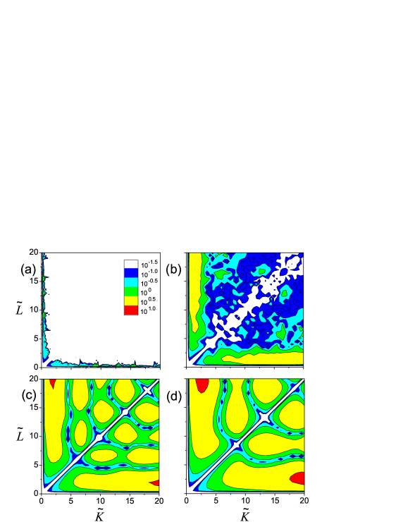
Figure 2: (Color online) (a): Absolute values of the classical current acceleration rate, denoted $\left|R_{c}\right|$, as a function of $\tilde{K}$ and $\tilde{L}$, for the RA model in the $\eta$-classical limit, Eq. (23). (b)-(d): Absolute values of the quantum current acceleration rate, denoted $\left|R_{q}\right|$, as a function of $\tilde{K}$ and $\tilde{L}$, for the RA model in Eq. (22), with (b) $\tilde{\hbar}=1$, (c) $\tilde{\hbar}=2\pi/3$, and (d) $\tilde{\hbar}=\pi$. In all the cases we set $\phi=\pi/2$. The contour scale $10^{-1.5}$ is for values less than $10^{-1.5}$, the contour scale $10^{-1.0}$ is for values between $10^{-1.5}$ and $10^{-1.0}$, and so on. The contour scales used in panel (a) apply to other panels as well.

Figure 2 shows the contour plots of $\left|R_{q}\right|$ and $\left|R_{c}\right|$ thus obtained as a function of $\tilde{K}$ and $\tilde{L}$. A number of interesting features can be observed from Fig. 2. First, significant classical ratchet acceleration (see Fig. 2a) exists only for those parameter regimes close to the $\tilde{K}$ axis or the $\tilde{L}$ axis. That is, at least one of the two values of $\tilde{K}$ and $\tilde{L}$ should be small for a considerable classical ratchet acceleration to emerge. But even that condition does not suffice. It is also clear from Fig. 2a that the regime of $\tilde{K}\sim\tilde{L}$ should be excluded in order to have an appreciable $\left|R_{c}\right|$. The overall result is that in the parameter space defined by $\tilde{K}$ and $\tilde{L}$, only a very small portion can yield considerable ratchet acceleration in the $\eta$-classical limit. Second, the quantum results shown in Fig. 2b-2d display many interest patterns. These patterns are absent in the classical case shown in Fig. 2a, and they vary strongly if we change $\tilde{\hbar}/\pi$ from an irrational value to a rational value. It can also be seen from Fig. 2b-2d that appreciable quantum ratchet acceleration occurs in a much larger parameter regime, often with $\left|R_{q}\right|>\left|R_{c}\right|$. Third, the quantum results share one feature with the classical result. That is, along the direction of $\tilde{K}=\tilde{L}$, $|R_{q}|$ is also seen to be small (typically much smaller than $10^{-1.5}$).

Some exceptions seem to be captured by Fig. 2b, where $\left|R_{q}\right|$ can become larger than $10^{-1.5}$ along the direction $\tilde{K}=\tilde{L}$. However, upon a careful investigation, we find that these exceptions are mainly caused by the particular way we numerically determine $R_{q}$. Indeed, if we follow the dynamics much longer (e.g. $10^{4}-10^{6}$ kicks), then the ratchet current tends to saturate for these exceptional cases, in contrast to the unbounded linear acceleration observed in other cases with $\tilde{K}\neq\tilde{L}$. Detailed investigations of such transient effects in the ratchet acceleration are beyond the scope this work. The exact boundary between bounded and unbounded quantum current acceleration can be an interesting and challenging mathematical problem.

Figure 3: The phase space portrait of the $\eta$-classical limit described by Eq. (23), for $2\tilde{L}=\tilde{K}=1$ in panel (a), $2\tilde{K}=\tilde{L}=1$ in panel (b), $\tilde{K}=\tilde{L}=1$ in panel (c), and $2\tilde{L}=\tilde{K}=4$ in panel (d). For all the panels we choose $\phi=\pi/2$. In cases (a) and (b) phase space invariant curves extended in the momentum space can be clearly seen. In case (c) there is a web of separatrix structures and phase space invariant curves along the momentum space no longer exist. Case (d) represents a fully chaotic phase space if both $\tilde{K}$ and $\tilde{L}$ are sufficiently large.

To shed more light on the results in Fig. 2, let us examine in Fig. 3 the phase space structures of the $\eta$-classical limit of our RA model. The phase space structure of the entire phase space is just an infinite repetition (in both $\tilde{q}^{c}$ and $\tilde{p}^{c}$) of what is shown in Fig. 3. If $\tilde{K}\neq\tilde{L}$ and either $\tilde{K}$ or $\tilde{L}$ is sufficiently small, then we always find phase space invariant curves extended in momentum. Trajectories moving along these invariant curves will display ballistic-like diffusion. Such a phase space feature differs from that of the standard kicked Harper model. In the latter case the phase space invariant curves can lie parallel to the $q^{c}$-axis if $\tilde{K}\ll\tilde{L}$. This difference is expected, because the $\eta$-classical Hamiltonian in Eq. (23) is a twisted version of the kicked Harper model.

Taking into account that $q^{c}=\pm\pi$ are equivalent points in the phase space, one can easily see that in both cases of Fig. 3a and Fig. 3b, there exist two bundles of phase space invariant curves, separated by a seperatrix structure associated with some unstable fixed points. Remarkably, the moving directions of the trajectories on the two bundles are opposite to each other. This feature is also consistent with the classical sum rule schanzprl . Based on these observations we are ready to explain the origin of the classical accelerating ratchet current. In particular, because the overlap of the $\tilde{p}^{c}=0$ line (the initial classical ensemble) with the two bundles of ballistic diffusion curves can be different, the effects of the two bundles of invariant curves cannot cancel out against each other and hence a net current develops. The current will increase linearly with time due to the ballistic nature of the phase space invariant curves extended in momentum. This understanding is found to be consistent with an estimate using the intersection lengths between the $\tilde{p}^{c}=0$ line and the two bundles of phase space invariant curves. This also clarifies the role of the parameter $\phi$. As is evident from the expression of the $\eta$-classical Hamiltonian in Eq. (23), the net effect of the parameter $\phi$ is a shift of the phase space structure along the $\tilde{p}^{c}$-axis. So the parameter $\phi$ can be used to tune the unbalanced overlap of the initial ensemble with the two bundles of phase space invariant curves.

By contrast, if $\tilde{K}=\tilde{L}$ (Fig. 3c), then before full chaos sets in, a web of separatrices emerge in the phase space and there are no longer phase space invariant curves extended in momentum. As the value of $\tilde{K}=\tilde{L}$ increases, the chaotic layer associated with the web of separatrices becomes thicker and thicker. During this regular-to-chaos transition no phase space invariant curves extended in momentum will emerge. As a result, so long as $\tilde{K}=\tilde{L}$, ballistic-like diffusion cannot happen and a linear acceleration of the ratchet current becomes impossible. This directly explains why the case of $\tilde{K}=\tilde{L}$ is so special for the $\eta$-classical ratchet acceleration. Figure 2 also shows the absence of significant quantum ratchet acceleration in cases of $\tilde{K}=\tilde{L}$. We believe that this quantum result is also due to the special classical phase space structure for $\tilde{K}=\tilde{L}$.

Let us finally discuss the fully chaotic cases. One typical example is shown in Fig. 3d. Analogous behavior can be found for other larger values of $\tilde{K}$ and $\tilde{L}$. Clearly, phase space invariant curves are all broken in these fully chaotic cases. As a result, classical ratchet acceleration necessarily vanishes, as illustrated in Fig. 1b. This rationalizes the main message from Fig. 2a, i.e., appreciable classical ratchet acceleration exists only for a small fraction of the parameter space of $\tilde{K}$ and $\tilde{L}$.

Remarkably, in general full classical chaos does not forbid quantum ratchet acceleration. As shown in Fig. 2b for a generic value of $\tilde{\hbar}$ (i.e., irrational with $\pi$), large $\left|R_{q}\right|$ can be found for relatively large $\tilde{K}$ and $\tilde{L}$, even when the associated $\eta$-classical dynamics becomes fully chaotic. A specific computational example has been shown in Fig. 1b. This hence confirms a similar observation made in Ref. Gongprl06 and constitutes another example of generic quantum violation of the classical sum rule schanzprl . In Ref. Gongprl06 , this violation was explained in terms of the concentration of quantum amplitudes on the remanents of classical cantori-like phase space structures extended in momentum. Here, as $\tilde{K}$ and $\tilde{L}$ increase, the two bundles of phase space invariant curves will also generate classical cantori-like structures. It can then expected that the classical cantori-like structures should be extended in the momentum space for $\tilde{K}<\tilde{L}$ as well as $\tilde{L}<\tilde{K}$. As such, the condition for quantum ratchet acceleration to occur in our new model should differ from that in Ref. Gongprl06 . Specifically, it is unnecessary to have a sufficiently large ratio $\tilde{K}/\tilde{L}$: a sufficiently small ratio $\tilde{K}/\tilde{L}$ should also do. Given this understanding, the quantum ratchet acceleration here with full classical chaos is expected to display a “dual” symmetry in the $\tilde{K}-\tilde{L}$ space. This is indeed the case: the pattern in Fig. 2b is symmetric along the line of $\tilde{K}=\tilde{L}$. Note also that for non-generic values of $\tilde{\hbar}/\pi$, the quantum ratchet acceleration rates as shown in Fig. 2c and Fig. 2d can be even larger, despite the fully chaotic phase space in the underlying $\eta$-classical limit.

Figure 4: (a) Dependence of the ratchet acceleration rate on the effective Planck constant $\tilde{\hbar}$ for $\phi=\pi/2$ (dotted line) and $\phi=1$ (solid line). (b) Dependence of the ratchet acceleration rate on the system parameter $\phi$, with $\tilde{\hbar}=\pi/2$ (dash-dotted line) and $\tilde{\hbar}=1$ (solid line). In all the cases here $3\tilde{L}=\tilde{K}=3\tilde{\hbar}$.

III.3 Dependence of Acceleration Rate on $\tilde{\hbar}$ and $\phi$

Focusing on the quantum case, here we first examine the dependence of $R_{q}$ on $\tilde{\hbar}$. As already indicated by the drastic differences between Fig. 2b, Fig. 2c, and Fig. 2d, one might wonder if $R_{q}$ is too sensitive to $\tilde{\hbar}$ such that experimental uncertainties in $\tilde{\hbar}$ may kill the ratchet acceleration altogether. To address this concern we show two typical computational results in Fig. 4a for two values of $\phi$. In both cases some sharp peaks of $R_{q}$ can be seen. These peaks are located at those values of $\tilde{\hbar}$ that are rational multiples of $\pi$. Nevertheless, the overall $\tilde{\hbar}$-dependence of $R_{q}$ does not show drastic oscillations. They can be varying smoothly over a considerably wide range of $\tilde{\hbar}$. This feature also resembles what is found in Ref. Gongprl06 . In the regime of very small $\tilde{\hbar}$, we have checked that $R_{q}$ does approach the $\eta$-classical acceleration rate $R_{c}$, thus establishing the expected quantum-classical correspondence. It should be stressed that the $\tilde{\hbar}$-dependence of $R_{q}$ shown here is a purely quantum effect. To have a theory accounting for this $\tilde{\hbar}$-dependence would be challenging but truly fascinating.

A related question is whether or not the ratchet acceleration is robust to variations in the parameter $\phi$ that characterizes the phase lag between two optical lattices of the same lattice constant. As demonstrated by the example shown in Fig. 4b, the $\phi$-dependence of $R_{q}$ is smooth in the entire range of $\phi$. This is somewhat expected: in the $\eta$-classical limit the parameter $\phi$ only shifts the phase space structure along the momentum axis. The conclusion is that small fluctuations in $\phi$ or $\tilde{\hbar}$ should not be a big concern for experimental studies.

III.4 Effects of the Quasi-Momentum Spread in Cold-Atom Experiments

In cold-atom experiments of kicked-rotor systems, the initial state cannot be exactly the state with zero quasi-momentum, even when the atoms are injected by a large-size Bose-Einstein condensate. Indeed, cold atoms are moving in real space, so their matter-wave state does not need to satisfy the periodic boundary condition inherent to a true kicked-rotor system. To motivate cold-atom experimental studies of our new RA model, it becomes necessary to examine the detrimental effects of the nonzero quasi-momentum spread in the initial state.

Because the kicking optical lattice potentials are always periodic, the quasi-momentum of the cold atoms, denoted $\beta$, is a conserved quantity danaprl ; quasimom . The dynamics emanated from an initial state with a spread in $\beta$ can then be easily simulated by considering each $\beta$-component separately. To shed more light on this issue let us return to the DKRM propagator $U_{\text{DKRM}}$ in Eq. (2). For each $\beta$ component, one now has $\tilde{p}|n\rangle=(n+\beta)|n\rangle$. This leads to the consequence that $e^{-iT\frac{p^{2}}{2\hbar}}\neq 1$ under the quantum resonance condition $T\hbar=4\pi$. Nevertheless, for $T\hbar=4\pi$ and for the potentials $V_{K}(q)$ and $V_{L}(q)$ used in our RA model, it is enlightening to rewrite Eq. (2) as

$${U}_{\text{RA}}^{\beta}=e^{-i2\pi\frac{\tilde{p}^{2}}{\tilde{\hbar}^{2}}}e^{i\frac{\tilde{p}^{2}}{2\tilde{\hbar}}}e^{-i\frac{\tilde{L}}{\tilde{\hbar}}\cos(q+\phi)}e^{-i\frac{\tilde{p}^{2}}{2\tilde{\hbar}}}e^{-i\frac{\tilde{K}}{\tilde{\hbar}}\cos(q)}.$$ (26)

Except for the first factor, this expression is completely parallel to $U_{\text{RA}}$ in Eq. (22). Because the first factor is no longer unity and changes with $\beta$, the first factor introduces de-phasing when a distribution of $\beta$ values are averaged over. Therefore, it can be expected that the $\beta$ spread will tend to saturate the accelerating ratchet current.

Below we assume a Gaussian distribution of $\beta$, with the variance denoted by $\Delta\beta$ and the mean value denoted by $\overline{\beta}$. Results for a typical case are shown in Fig. 5. It is seen from Fig. 5a that a nonzero variance $\Delta\beta$ indeed induces the saturation of the quantum ratchet current. The exact saturation time increases, but slowly, with decreasing $\Delta\beta$. For the parameters adopted in Fig. 5a, the typical saturation time is around 20 kicking periods for $\Delta\beta\sim 0.002$ (scaled by $\tilde{\hbar}$), a characteristic value of the $\beta$ spread reported in a recent experiment using Bose-Einstein condensates ryu . Figure 5b also shows an interesting dependence of the ratchet current at $t=7T$ upon the mean quasi-momentum $\overline{\beta}$ of the initial state. The result for $\Delta\beta=0.01$ is seen to be almost the same as that for $\Delta\beta=0.002$. This $\overline{\beta}$-dependence of the ratchet current at early times might be of interest to experimental studies as well.

In future experiments the quasi-momentum spread can be made smaller than $\Delta\beta\sim 0.002$ ryu . However, the result in Fig. 5a indicates that even for $\Delta\beta\sim 0.0005$, the saturation still sets in within a relatively short time scale. Interestingly, a previous theoretical RA model using a bichromatic optical lattice displays saturation at a similar time scale kenfack . This indicates that when faced with the detrimental effects of the quasi-momentum spread, the robustness of our new RA model without a bichromatic optical lattice is similar to previous models with bichromatic optical lattices.

Figure 5: Effects of the quasi-momentum spread on quantum ratchet currents with $\tilde{\hbar}=1$, $2\tilde{L}=\tilde{K}=2$, $\phi=\pi/2$. $\Delta\langle\tilde{p}(t)\rangle\equiv\langle\tilde{p}(t)\rangle-\langle\tilde{p}(0)\rangle$. In panel (a), $\overline{\beta}=0$ and the variance in $\beta$ is given by $\Delta\beta=0,0.0005,0.001,0.002$ and $0.004$ (from above to bottom). In panel (b), $\Delta\langle\tilde{p}(t)\rangle$ at $t=7$ with $\Delta\beta=0.002$ (dashed line) and $0.01$ (solid line) are shown as a function of the mean quasi-momentum $\overline{\beta}$ of the initial state.

IV Double-kicked rotor systems on high-order quantum resonances

So far we have studied the ratchet transport in the DKRM under the main quantum resonance condition $T\hbar=4\pi$. To motivate both theoretical and experimental studies in the future, in this short section we briefly discuss an interesting extension of the current study. The extension is about the dynamics of ratchet current acceleration in DKRM on high-order quantum resonances. In such extended cases, $T\hbar=4\pi\nu/\mu$, where $\nu$ and $\mu$ are two incommensurate integers. Under this high-order quantum resonance condition we find that analogous ratchet acceleration can be obtained as well, without using a bichromatic optical lattice. Thus, ratchet current acceleration itself may provide a useful tool for studies of high-order quantum resonances in DKRM.

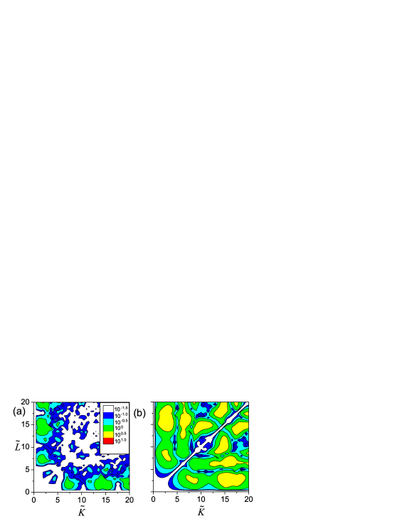
Figure 6: (Color online) Absolute values of the ratchet current acceleration rate, $|{R}_{q}|\equiv\left|d\langle\tilde{p}\rangle/dt\right|$, for a double kicked rotor system at quantum anti-resonance $T\hbar=2\pi$. The quantum propagator is given by Eq. (2). For the sake of comparison, the same parameter rescaling as in the cases of DKRM under the main quantum resonance is adopted. The rescaled parameters are given by $\tilde{\hbar}=1$ in panel (a), and $\tilde{\hbar}=2\pi/3$ in panel (b). In both cases $\phi=\pi/2$. The meaning of the contour scale is the same as in Fig. 2, and the contour scales used in panel (a) apply to panel (b) as well.

As an example in Fig. 6 we show $\left|R_{q}\right|$ under the quantum anti-resonance condition $T\hbar=2\pi$, as a function of $\tilde{K}$ and $\tilde{L}$. The kicking potentials $V_{K}(q)$ and $V_{L}(q)$ are the same as those considered in Figs. 1-5. The case in Fig. 6a represents cases with a generic value of $\tilde{\hbar}$, yielding appreciable $\left|R_{q}\right|$ in some regimes. In this case the detailed dependence of $\left|R_{q}\right|$ on $\tilde{K}$ and $\tilde{L}$ is seen to be rather complicated. The case of $\hbar=2\pi/3$ in Fig. 6b represents cases with nongeneric values of $\tilde{\hbar}$. The associated ratchet acceleration effect is seen to be larger over a wider regime. The dependence of $\left|R_{q}\right|$ on $\tilde{K}$ and $\tilde{L}$ is also simpler than that seen in Fig. 6a. These results have no apparent connections with classical ratchet transport, in the sense that for high-order quantum resonances we can no longer define an $\eta$-classical limit to guide our qualitative understandings. However, as is evident from Fig. 6, even in these quantum anti-resonance DKRM cases, a significant ratchet acceleration rate also requires the condition $\tilde{K}\neq\tilde{L}$. More studies of this extension will be carried out in the near future.

V Concluding Remarks

To conclude, we have proposed and studied a new quantum ratchet accelerator model based on atom optics realizations of kicked-rotor systems. Unlike all previous ratchet accelerator models, here we do not need to use a bichromatic optical lattice potential. Based on this advantage and the detailed computational studies presented here, we believe that the cold-atom realization of our ratchet accelerator model is within the reach of today’s state-of-the-art experiments sadgrove ; danaprl . Indeed, the avenue of using atom optics to experimentally study a whole class of kicked-Harper-like models has been just opened up jiaopra08 , and the ratchet accelerator model proposed here seems to be a wonderful starting point along this direction.

To have a linear acceleration of ratchet current in the $\eta$-classical limit of our model, we have shown that the phase space invariant curves extended in the momentum space are a necessary condition. Therefore, for kicking optical lattice potentials $K\cos(q)$ and $L\cos(q+\phi)$, an on-resonance double-kicked rotor with equal kicking amplitudes $K$ and $L$ cannot yield an unbounded and linearly increasing classical current. Instead, we need unequal kicking amplitudes for accelerating and unbounded classical current to occur. This interesting requirement is also observed, but not fully explained, in the quantum dynamics. Given unequal kicking amplitudes, the quantum ratchet acceleration in our model can however persist for large kicking amplitudes, even when the $\eta$-classical limit no longer has phase space invariant curves extended in the momentum space. This purely quantum effect is believed to be another example that remanents of classical phase space structures can dramatically impact the quantum dynamics. Considering these insights, we hope that our simple ratchet accelerator model will also motivate future theoretical work to better understand quantum transport and quantum-classical correspondence in classically chaotic systems.

- (1) J.B. Gong and P. Brumer, Phys. Rev. E70, 016202 (2004); Annu. Rev. Phys. Chem. 56, 1 (2005).
- (2) H. Schanz, M.F. Otto, R. Ketzmerick, and T. Dittrich, Phys. Rev. Lett. 87, 070601 (2001).
- (3) T.S. Monteiro, P.A. Dando, N.A.C. Hutchings, and M.R. Isherwood, Phys. Rev. Lett. 89, 194102 (2002).
- (4) T. Cheon, P. Exner, and P. Seba, J. Phys. Soc. Jpn. 72, 1087 (2003).
- (5) H. Schanz, T. Dittrich, and R. Ketzmerick, Phys. Rev. E71, 026228 (2005).
- (6) S. Kohler, J. Lehmann, and P. Hänggi, Phys. Rep. 406, 379 (2005).
- (7) S. Denisov, L. Morales-Molina, S. Flach, and P. Hänggi, Phys. Rev. A75, 063424 (2007).
- (8) E. Lundh and M. Wallin, Phys. Rev. Lett. 94, 110603 (2005).
- (9) A. Kenfack, J.B. Gong, and A.K. Pattanayak, Phys. Rev. Lett. 100, 044104 (2008).
- (10) G. Casati and B.V. Chirikov, Quantum Chaos: between order and disorder (Cambridge University Press, New York, 1995).
- (11) G. Ritt et al., Phys. Rev. A74, 063622 (2006); T. Salger et al., Phys. Rev. Lett. 99, 190405 (2007).
- (12) M. Sadgrove, M. Horikoshi, T. Sekimura, and K. Nakagawa, Phys. Rev. Lett. 99, 043002 (2007).
- (13) I. Dana, V. Ramareddy, I. Talukdar, and G. S. Summy, Phys. Rev. Lett. 100, 024103 (2008).
- (14) D. Poletti, G.C. Carlo, and B. Li, Phys. Rev. E75, 011102 (2007).
- (15) T. Geisel, R. Ketzmerick, and G. Petschel, Phys. Rev. Lett. 67, 3635 (1991); R. Lima and D. Shepelyansky, ibid. 67, 1377 (1991); R. Artuso et al., ibid. 69, 3302 (1992); R. Ketzmerick, K. Kruse, and T. Geisel, ibid. 80, 137 (1998); I.I. Satija, Phys. Rev. E66, 015202 (2002).
- (16) J.B. Gong and P. Brumer, Phys. Rev. Lett. 97, 240602 (2006).
- (17) J. Wang and J.B. Gong, Phys. Rev. A77, 031405(R) (2008).
- (18) J. Wang, A.S. Mouritzen, and J.B. Gong, J. Mod. Opt. (in press). See also ArXiv 0803.3859.
- (19) P.H. Jones, M.M. Stocklin, G. Hur, and T.S. Monteiro, Phys. Rev. Lett. 93, 223002 (2004).
- (20) C.E. Creffield, G. Hur, T.S. Monteiro, Phys. Rev. Lett. 96, 024103 (2006); C.E. Creffield, S. Fishman, T.S. Monteiro, Phys. Rev. E. 73, 066202 (2006).
- (21) J. Wang, T.S. Monteiro, S. Fishman, J.P. Keating, and R. Schubert, Phys. Rev. Lett. 99 234101 (2007).
- (22) S. Wimberger, I. Guarneri, and S. Fishman, Nonlinearity 16, 1381 (2003); I. Dana and D.L. Dorofeev, Phys. Rev. E 73, 026206 (2006); ibid. 74, 045201(R) (2006); M. Saunders, P.L. Halkyard, K.J. Challis, and S.A. Gardiner, Phys. Rev. A76, 043415 (2007).
- (23) J.B. Gong and J. Wang, Phys. Rev. E76, 036217 (2007).
- (24) S. Fishman, I. Guarneri and L. Rebuzzini, Phys. Rev. Lett. 89, 084101 (2002).
- (25) I. Dana, Phys. Lett. A 197, 413 (1995).
- (26) G.G. Carlo et al., Phys. Rev. A74, 033617 (2006).
- (27) C. Ryu et al., Phys. Rev. Lett. 96, 160403 (2006).