An AzTEC 1.1 mm Survey of the GOODS-N Field I: Maps, Catalogue, and Source Statistics

Abstract

We have conducted a deep and uniform 1.1 mm survey of the GOODS-N field with AzTEC on the James Clerk Maxwell Telescope (JCMT). Here we present the first results from this survey including maps, the source catalogue, and 1.1 mm number-counts. The results presented here were obtained from a 245 arcmin² region with near uniform coverage to a depth of 0.96–1.16 mJy beam^-1. Our robust catalogue contains 28 source candidates detected with S/N $\geq 3.75$, only $\sim$1–2 of which are expected to be spurious detections. Of these source candidates, 8 are also detected by SCUBA at 850 $\mu$m in regions where there is good overlap between the two surveys. The major advantage of our survey over that with SCUBA is the uniformity of coverage. We calculate number counts using two different techniques: the first using a frequentist parameter estimation, and the second using a Bayesian method. The two sets of results are in good agreement. We find that the 1.1 mm differential number counts are well described in the 2–6 mJy range by the functional form $dN/dS=N^{\prime}(S^{\prime}/S)\mathrm{exp}(-S/S^{\prime})$ with fitted parameters $S^{\prime}=1.25\pm 0.38$ mJy and $dN/dS=300\pm 90$ mJy^-1 deg^-2 at 3 mJy.

1 Introduction

Identifying and studying the galaxies at high redshift that will evolve into today’s normal and massive galaxies remains a major goal of observational astrophysics. Galaxies discovered in deep sub-millimetre and mm-wavelength surveys (e.g. Smail et al., 1997; Hughes et al., 1998; Barger et al., 1998; Blain et al., 1999; Barger et al., 1999; Eales et al., 2000; Cowie et al., 2002; Scott et al., 2002; Webb et al., 2003; Borys et al., 2003; Greve et al., 2004; Laurent et al., 2005) are generally thought to be dominated by dusty, possibly merger-induced starburst systems and active galactic nuclei (AGN) at redshifts $z>2$ with star formation rates as high as SFR $\sim 1000~{}\mathrm{M}_{\sun}\mathrm{yr}^{-1}$ (Blain et al., 2002). The high areal number density of these sub-mm and mm-detected galaxies (SMGs), combined with their implied high star formation rates and measured FIR luminosities ($L_{\mathrm{FIR}}\sim 10^{12}\mathrm{L}_{\sun}$, Kovács et al., 2006; Coppin et al., 2008), makes their estimated contribution to both the global star formation density and the sub-mm background radiation as high as 50% at $z\sim 2$ (e.g., Borys et al., 2003; Wall et al., 2008). Their observed number counts imply strong evolution between $z=2$ and today (e.g. Scott et al., 2002; Greve et al., 2004; Coppin et al., 2006). The high star formation rates at early epochs of SMGs generally match the expectation for rapidly forming elliptical galaxies, a view supported by the high rate of mergers seen locally in samples of ultra-luminous infrared galaxies (ULIRGs; Borne et al., 2000), which are plausible local counterparts of distant SMGs. Together, these characteristics have led many observers to surmise that SMGs are likely to evolve into the massive galaxies observed locally (e.g., Dunlop et al., 1994; Smail et al., 1997; Bertoldi et al., 2007) and may hold important clues to the processes of galaxy and structure formation in general at high redshift.

GOODS-N is one of the most intensively studied extragalactic fields, with deep multi-wavelength photometric coverage from numerous ground-based and space-based facilities. These include Chandra in the X-ray (Alexander et al., 2003), HST in the optical and NIR (Giavalisco et al., 2004), Spitzer in the NIR–MIR (Chary et al. in prep., Dickinson et al. in prep.), and the Very Large Array in the radio (Richards, 2000, Morrison et al. in prep.), as well as highly complete spectroscopic surveys from ground-based observatories (e.g. Wirth et al., 2004; Cowie et al., 2004). This field is therefore ideally suited for deep mm-wavelength studies of SMGs: the extensive coverage in GOODS-N allows the identification of SMG counterparts in X-ray, UV, optical, IR, and radio bands, as well as constraints on photometric redshifts and investigation of SMG power sources and evolution.

Deep mm surveys of blank fields are needed in order to constrain the faint end of the SMG number counts, while large areal coverage is required to constrain the bright end. Together they provide strong constraints on evolutionary scenarios. Previous sub-mm surveys of GOODS-N have been carried out with SCUBA on the JCMT (Hughes et al., 1998; Barger et al., 2000; Borys et al., 2003; Wang et al., 2004; Pope et al., 2005). The ‘Super-map’ of the GOODS-N field, which was assembled from all available JCMT shifts covering the field, contains 40 robust sources at 850 $\mu$m down to an average sensitivity of 3.4 mJy ($1\sigma$) and covers 200 arcmin² (Borys et al., 2003; Pope et al., 2005). However, the r.m.s. is highly non-uniform ranging from 0.4 mJy to 6 mJy (see Fig. 1). That non-uniformity presents serious complications for comparisons with multi-wavelength data.

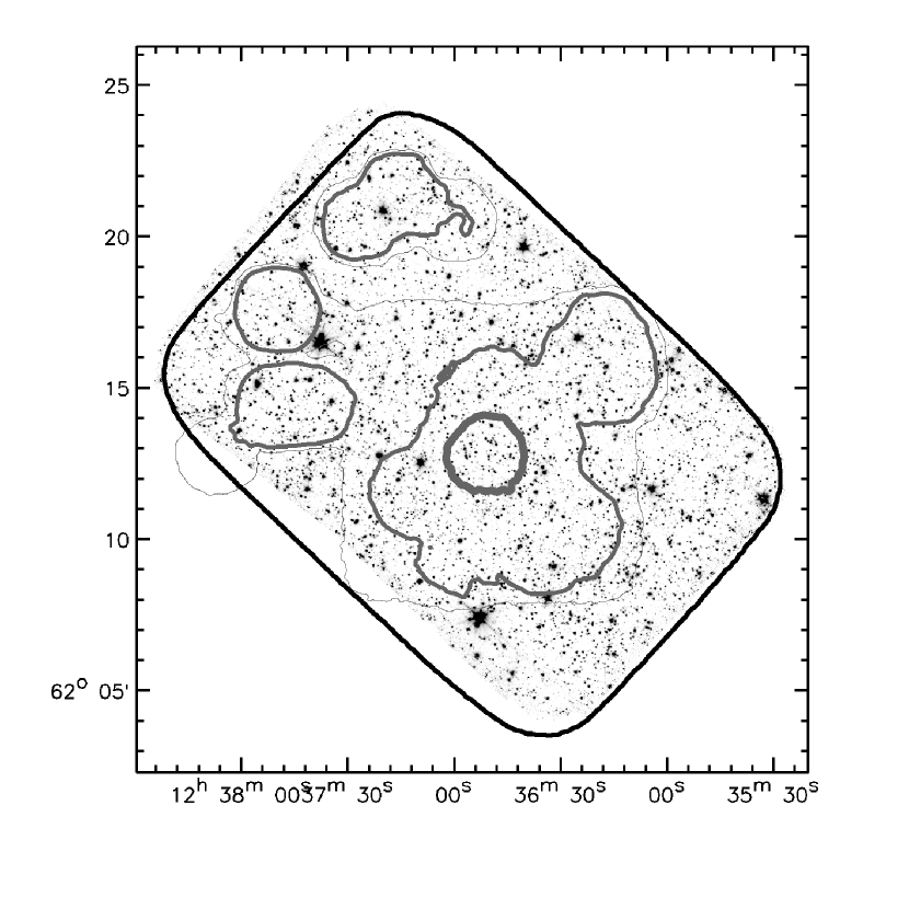
Figure 1: AzTEC and SCUBA coverage contours for the GOODS-N region demonstrates our uniform coverage. The dark rectangular contour corresponds to the AzTEC region with a map r.m.s. $\leq$1.16 mJy at 1.1 mm, the coverage region presented here. The grey contours, according to increasing line thickness, are the 850 $\mu$m SCUBA contours for r.m.s. values of 4 mJy, 2.5 mJy, and 0.5 mJy respectively. The underlying map is the IRAC 3.6 $\mu$m image from the Spitzer legacy program (Dickinson et al. in prep). The AzTEC map represents a significant improvement in the uniformity of coverage at faint flux levels.

In this paper we present a new 1.1 mm survey of the GOODS-N field made with AzTEC (Wilson et al., 2008) at the 15-m James Clerk Maxwell Telescope (JCMT) on Mauna Kea, Hawaii. This map is the deepest blank-field survey undertaken during the AzTEC/JCMT observing campaign, and is one of the largest, deepest, and most uniform mm-wavelength maps of any region of the sky. Our map covers $245$ arcmin² and completely encompasses the $16.5^{\prime}\times 10^{\prime}$ Spitzer GOODS-N field and all of the previous GOODS-N sub-mm and mm-wavelength fields, including the original HDF map of Hughes et al. (1998) and the SCUBA GOODS-N ‘Super-map’ (indicated in Fig. 1 here and presented in Borys et al., 2003; Pope et al., 2005). The large number and high stability of the AzTEC bolometers has enabled us to produce a map with small variations in r.m.s., from 0.96–1.16 mJy, across the 245 min² field. This uniformity is a drastic improvement over the SCUBA GOODS-N ‘Super-map.’ The sensitivity variations of the AzTEC and SCUBA maps are compared in Fig. 1.

In this work, we extract a catalogue of mm sources from the map and calculate number counts towards the faint end of the 1.1-mm galaxy population. The main results we discuss here were obtained from the AzTEC data alone; data from other surveys have been used only as tools to check the quality of our map. A second paper will address counterpart identification of our AzTEC sources at other wavelengths (Chapin et al. in prep.). We present the JCMT/AzTEC observations of GOODS-N in § 2, data reduction and analysis leading to source identification in § 3, properties of our source catalogue in § 4, the number counts analysis in § 5, the discussion of results in § 6, and the conclusion in § 7.

2 AZTEC OBSERVATIONS OF GOODS-N

AzTEC is a 144-element focal-plane bolometer array designed for use at the 50-m Large Millimetre Telescope (LMT) currently nearing completion on Cerro La Negra, Mexico. Prior to permanent installation at the LMT, AzTEC was used on the JCMT between Nov. 2005 and Feb. 2006, primarily for deep, large-area blank field SMG surveys (e.g. Scott et al., 2008, Austermann et al. in prep.). We imaged the GOODS-N field at $1.1\,$mm with the AzTEC camera during this 2005–2006 JCMT observing campaign. Details of the AzTEC optical design, detector array, and instrument performance can be found in Wilson et al. (2008). Each detector has a roughly Gaussian-shaped beam on the sky with an 18-arcsec full-width at half-maximum (FWHM). Given the beam separation of 22 arcsec, the hexagonal close-packed array subtends a “footprint” of 5 arcmin on the sky. Out of the full array complement of 144 bolometer-channels, 107 were operational during this run.

We mapped a 21 arcmin $\times$ 15 arcmin area centred on the GOODS-N field (12^h37^m00^s, +62^∘13′00″) in unchopped raster-scan mode, where the primary mirror scans the sky at constant velocity, takes a small orthogonal step, then scans with the same speed in the opposite direction, repeating until the entire area has been covered. We used a step size of 9 arcsec in order to uniformly Nyquist-sample the sky. We scanned at speeds in the range 60 arcsec s^-1–180 arcsec s^-1 as allowed by the fast time constants of our micro-mesh bolometers, with no adverse vibrational systematics. In total, we obtained 50 usable individual raster-scan observations, each taking 40 minutes (excluding calibration and pointing overheads). The zenith opacity at 225 GHz is monitored with the CSO tau meter, and ranged from 0.05–0.27 during the GOODS-N observations. This corresponds to 1.1 mm transmissions in the range 70–94%. A detailed description and justification of the scan strategy we used can be found in Wilson et al. (2008).

3 Data Reduction: from time-streams to source catalogue

In this section, we summarise the processing of the AzTEC/GOODS-N data, which is specifically geared towards finding mm point sources. The data reduction procedure generally follows the method outlined in Scott et al. (2008), although we emphasise several new pieces of analysis that were facilitated by the improved depth of this map over the COSMOS survey. We begin with the cleaning and calibration of the time-stream data in § 3.1, which includes a new investigation into the sample length over which to clean the data. In § 3.2, we describe the map making process and the optimal filtering for point sources. We asses the properties and quality of the AzTEC/GOODS-N map in § 3.3. The depth of this survey has enabled us to ascertain the degree to which our data follow Gaussian statistics and detect, directly, a departure from it at long integration times indicating a component of signal variance due to source confusion. The astrometry of the map is analysed in § 3.4, and we describe the extraction of sources from the optimally filtered map in § 3.5.

3.1 Filtering, cleaning, and calibration of time-stream data

The AzTEC data for each raster-scan observation consists of pointing, housekeeping (internal thermometry, etc.), and bolometer time-stream signals. Because the bolometer data are sampled at 64 Hz, all other signals are interpolated to that frequency as needed by the analysis. The raw time-streams of the 107 working bolometers are first despiked and low-pass filtered at 16 Hz, as described in Scott et al. (2008). The despiked and filtered time-streams are next “cleaned” using a principal component analysis (PCA) approach, which primarily removes the strong atmospheric signal from the data. This “PCA-cleaning” method was developed by the Bolocam group (Laurent et al., 2005) and later adapted for AzTEC, as described in Scott et al. (2008). As explained there, we also generate PCA-cleaned time streams corresponding to a simulated point source near the field centre, in order to produce the point-source kernel, which is used later for beam-smoothing our maps (see § 3.2).

In this work we go beyond the analysis in Scott et al. (2008) to verify that we have made good choices with regard to several aspects of the general cleaning procedure that has been adopted for all of the existing AzTEC data. We examine two outstanding questions in particular: 1) does PCA-cleaning work better than a simple common-mode subtraction based only on the average signal measured by all detectors as a function of time? and 2) over what time scale should each eigenvector projection be calculated in order to give the best results?

The first question addresses whether simple physical models may be used in place of PCA-cleaning, where the choice of which modes to remove from the data is not physically motivated. We investigate this by creating a simple sky-signal template as the average of all of the detectors at each time sample. We then fit for an amplitude coefficient of the template to each detector by minimising the r.m.s. between the scaled template and the actual data. This scaled template is removed from the bolometer data and we examine the residual signal, which ideally consists only of astronomical signal and white noise. We find that this residual signal contains many smaller detector-detector correlations that are clearly visible in the data and are dominant compared to the signal produced by astronomical sources in the map. The residual time-stream r.m.s. from the simple sky-template subtraction is usually about twice the r.m.s. resulting from PCA cleaning. This test shows that the simple common-mode removal technique is insufficient.

In the “standard” PCA-cleaning procedure for AzTEC data, outlined in Scott et al. (2008), the eigenvector decomposition is performed on each scan ($\sim 5$–15 s of data). We now study which time scales give the best results using a statistical correlation analysis. We generate a bolometer-bolometer Pearson correlation matrix using sample lengths that range from a fraction of a second to tens of minutes (the length of a complete observation). On the shortest time scales, the correlation coefficients have large uncertainties due to sample variance (too few samples from which to make estimates). On time scales corresponding to a single raster-scan ($\sim$5–15 sec), however, the sample variance decreases and a clear pattern emerges: the strength of the correlations drops off uniformly with physical separation between the detectors. The most obvious trend is the gradient in correlations that we see with detector elevation, which is presumed to be produced by the underlying gradient in sky emission. As the sample length increases, a different pattern emerges, in which the dominant correlation appears to be related to the order in which the detectors are sampled by the read-out electronics, rather than their physical separation. These correlations, likely due to electronics-related $1/f$ drifts, are effectively removed when using scan-sized sample lengths (5–15 s) as well, since they appear as DC baseline differences on these short time-scales. These results verify that scan-sized sample lengths produce the best results as they provide a sufficient number of samples on short enough time scales.

After PCA-cleaning the bolometer signals, we apply a calibration factor to convert the bolometers’ voltage time-streams into units of Jy per beam. Details of this procedure are given in Wilson et al. (2008). The total error on the calibrated signals (including the error on the absolute flux of Uranus) is 11%.

3.2 Map-making and optimal filtering

The map-making process used to generate the final optimally filtered AzTEC/GOODS-N map is identical to that used in Scott et al. (2008), and the reader is directed to that paper for the details of this process, which we briefly summarise below.

We first generate maps for each of the 50 individual raster-scan observations separately by binning the time-stream data onto a 3″ $\times$ 3″ grid in RA-Dec which is tangent to the celestial sphere at (12^h37^m00^s, +62^∘13′00″). We chose the same tangent point and pixel size as that used for the SCUBA map of GOODS-N (see for example Pope et al., 2006) so that the two maps can easily be compared in a future paper. We find that this pixel size provides a good compromise between reducing computation time, while sampling with high resolution the 18-arcsec FWHM beams. Individual signal maps and their corresponding weight maps for each observation are created as described in Scott et al. (2008), along with kernel maps that reflect how a faint point source is affected by PCA-cleaning and other steps in the analysis. Next, we form a single “co-added” signal map from the weighted average over all 50 individual observations. An averaged kernel map is also created in a similar way. The total weight map is calculated by summing the weights from individual observations, pixel by pixel. As described by Scott et al. (2008) we also generate 100 noise realization maps corresponding to the co-added map.

We then use a spatial filter to beam-smooth our map using the point-source kernel, by optimally weighting each spatial-frequency component of this convolution according to the spatial power spectral density (PSD) of noise-realization maps. Details of this optimal filter can also be found in Scott et al. (2008).

3.3 Map quality: depth, uniformity, point-source response, and noise integration

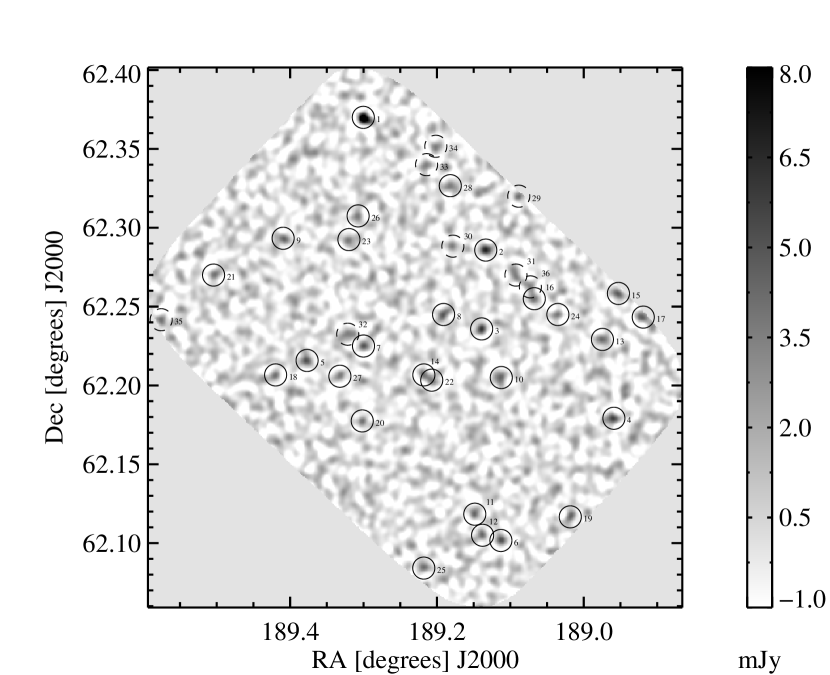
Figure 2: AzTEC/GOODS-N signal map with the 36 S/N$\geq$3.5 source candidates circled. Information about these source candidates is given in Table 1. Here and in that table, source candidates are numbered in decreasing order of S/N. The source candidates marked with dashed-line circles do not belong to the robust sub-list, indicated by a horizontal line in Table 1. The map has been trimmed to show only the 70% coverage region (245 arcmin²).

The final co-added, optimally filtered signal map for the GOODS-N field is shown in Fig. 2. Of the 315-arcmin² solid angle scanned by the telescope boresight during our survey, we expect $\sim$250 arcmin² to be imaged uniformly by the complete AzTEC array. We identify this region by imposing a coverage cut. We find that weights within 70% of the central value occur in a contiguous region of 245 arcmin². The map of Fig. 2 has been trimmed to only show this region. Much of the analysis presented here is limited to this region, which we will henceforth refer to as the the “70% coverage region.” The 1-$\sigma$ flux-density error estimates in the trimmed map range from 0.96 mJy beam^-1 in the centre to 1.16 mJy beam^-1 at the edges.

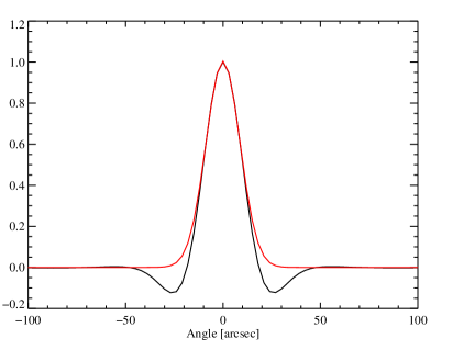
Figure 3: Cross section of the point-source kernel. The Gaussian that best fits the inner $R=10$ arcsec region is shown in the lighter shade and has a FWHM of 19.5 arcsec. The negative ring around the centre and other peripheral features (not visible here) are induced by PCA-cleaning as well as the optimal filter.

We also run the co-added kernel map through the same filtering process as the signal map. The resulting filtered kernel map, whose profile is shown in Fig. 3, is our best approximation of the shape of a point source in the co-added, filtered signal map. As demonstrated in § 3.4, our pointing jitter/uncertainty has a sub-2-arcsec characteristic scale; this will have little impact on the kernel shape and therefore is not included in generating the kernel map. The negative troughs around the central peak are due to a combination of array common-mode removal in the PCA-cleaning and de-weighting of longer spatial wavelength modes by the optimal filter. The point-source kernel also has radial scan-oriented features, or “spokes,” due to PCA cleaning that are $<$0.1% of the kernel amplitude. The directions of these spokes would vary across the map as the scan angle changes with RA-Dec. Therefore, the kernel map accurately reflects these spokes only for point sources near the centre of the field. However, because it is difficult to analytically model a point source (through PCA cleaning and optimal filtering) and because the radial features are very faint, we use the kernel map as a point source-template for injection of sources in the simulations described later.

Because this GOODS-N survey is the deepest blank-field survey conducted thus far with AzTEC on the JCMT, we demonstrate in Fig. 4 how the map noise averages down with the successive co-addition of individual observations. The central 200″$\times$200″ region of the signal map and the noise realisation maps are used for this calculation. The x-axis represents the average weight of a 3-arcsec pixel in this region prior to filtering. A scale factor converts this raw weight to an effective time, $T^{*}$, so that the final effective time equals the final integration time devoted to an average 3-arcsec pixel in this central patch. Thus, the increment in $T^{*}$ gained with the addition of an individual observation is the effective integration time contributed by that particular observation to the central region. The $i$th y-axis value is calculated by co-adding (averaging) individual signal maps from observations 1 through $i$, then applying the optimal filter, and finally taking the standard deviation of this co-added, filtered map in the central region. The crosses represent the signal map. The 100 curves shown in a lighter shade are calculated by carrying out the same process on 100 noise realisations. In the absence of systematics or astronomical signal, we expect all curves to scale as $1/\sqrt{T^{*}}$, in accordance with Gaussian statistics, as indicated by the dashed line. At higher $T^{*}$, we may expect a slight steepening in all curves because later co-additions better reflect our assumptions of circular symmetry (in the optimal filtering process) as we add more scan directions to the mix. However, this effect appears to be unmeasurably small in our data.

While the noise realisations follow the $1/\sqrt{T^{*}}$ trend, the signal map initially follows it but flattens near the point where ${\sim}20$–30 s of effective time is spent on a 3-arcsec pixel. Switching the order in which signal maps are co-added does not alter this trend or the noisy behaviour of these points at large $T^{*}$. Therefore, we conclude that: 1) single individual observations yield maps that are consistent with our noise realisations; 2) map features that do not survive scan-by-scan “jack-knifing,” presumably astronomical signal due to source confusion, prevent the signal map’s r.m.s. from improving as $1/\sqrt{T^{*}}$; and 3) the fact that noise realisations continue to follow this trend indicates that we are far from a systematics floor due to atmospheric or instrumental effects, even at the highest $T^{*}$.

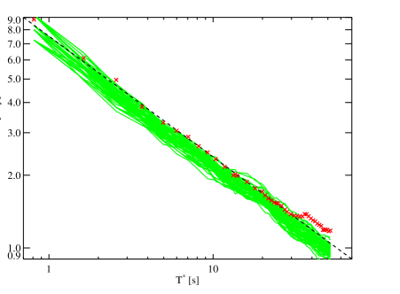
Figure 4: Behaviour of the signal map’s r.m.s. (crosses), as well as the r.m.s. of 100 separate noise realisations (collection of curves), as a function of the mean effective integration time $T^{*}$ spent on each 3-arcsec central pixel of map. The dashed curve shows the 1/$\sqrt{T^{*}}$ relationship expected in the absence of systematics and astronomical signal. This demonstrates how the map noise averages down with the successive addition of more observations. The “flattening” of the central r.m.s. at large $T^{*}$ in the signal map, compared to the noise maps, is due to astronomical signal. The fluctuations of this curve at large $T^{*}$ are simply due to noise in the r.m.s. itself, as re-ordering observations gives similar features near the same region.

3.4 Astrometry calibration

The pipeline used to produce this map of GOODS-N interpolates pointing offsets inferred from regular observations of pointing calibrators interspersed with science targets (Wilson et al., 2008; Scott et al., 2008). In order to verify the quality of this pointing model for GOODS-N, both in an absolute sense, and in terms of small variations between passes, we compare the AzTEC map with the extremely deep 1.4 GHz VLA data in this field (Richards, 2000, Morrison et al. in prep.). The radio data reduction and source list used here is the same as that of Pope et al. (2006), with a 1-$\sigma$ noise of $\sim$5.3 $\mu$Jy at the phase centre. The catalogue is constructed with a 4-$\sigma$ cut, and has positional uncertainties $\sim 0.2^{\prime\prime}$ (Morrison et al. in prep.).

We stack the signal in the AzTEC map at the positions of radio sources to check for gross astrometric shifts in the AzTEC pointing model, as well as any broadening in the stacked signal which may indicate significant random offsets in the pointing between visits. A more detailed comparison between the mm and 1.4 GHz map is presented in (Chapin et al. in prep.) to assist with the MIR/NIR identifications of individual AzTEC SMGs, and the production of radio–NIR SEDs.

The stack was made from the 453 1.4 GHz source positions that are within the uniform noise region of the AzTEC map. As in Scott et al. (2008) we check for an astrometric shift and broadening by fitting a simple model to the stacked image, which consists of an astrometric shift ($\delta$RA, $\delta$Dec) to the ideal point source kernel, convolved with a symmetric Gaussian with standard deviation $\sigma_{\rm p}$. This Gaussian represents our model for the random pointing error in the AzTEC map. We determine maximum likelihood estimates $\delta$RA $=0.2^{\prime\prime}$, $\delta$Dec $=-0.9^{\prime\prime}$, and $\sigma_{\rm p}=0.6^{\prime\prime}$. The expected positional uncertainty (in each coordinate) for a point source with a purely Gaussian beam is approximately $0.6\times$FWHM/(S/N) (see the Appendix in Ivison et al., 2007) where the FWHM is 18 arcsec in our case. The S/N of our stack is approximately 10, so the expected positional uncertainty is ${\sim}\,1^{\prime\prime}$. Therefore the total astrometric shift measured by the fitting process, $0.9^{\prime\prime}$, is consistent with the hypothesis that there is no significant underlying shift. We also note that the $\chi^{2}$ function for this fit is extremely shallow along the $\sigma_{\rm p}$ axis, so although the minimum occurs at $0.6^{\prime\prime}$, it is not significantly more likely than $0^{\prime\prime}$. We therefore conclude from this analysis that there is no significant offset, nor beam broadening caused by errors in the pointing model.

3.5 Source finding

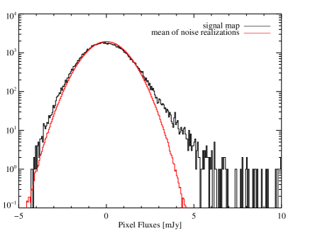
Figure 5: Pixel flux histogram of the final signal map in a dark shade and the average pixel flux histogram made from 100 noise realizations in a lighter shade. The positive tail and smaller negative excess in the signal map is due to the presence of point sources.

To investigate the presence of astronomical sources in our map, we plot in Fig. 5 a histogram of pixel fluxes in the 70% coverage region of the field. Also shown in a lighter shade is the average pixel histogram made from the 100 noise-realization maps. The noise histogram can be modelled well by a Gaussian centred on $0\,$mJy with a standard deviation of 1.0 mJy. The obvious excess of large positive pixel values and the small excess of negative values in the signal map are caused by the presence of sources.

To identify individual point sources, we first form a S/N map by multiplying the final (i.e. co-added and filtered) signal map by the square-root of the weight map. We then identify local maxima in this S/N map with S/N $\geq 3.5$. There are 36 local maxima that meet this condition in the 70% coverage region of the field. Our analysis of these source candidates is simplified because no pair of them are close enough to significantly alter each other’s recovered flux densities ($>$36 arcsec apart in each case). We have evidence that AzGN01 is a blend of two sources. However, since this knowledge is not based on AzTEC data alone, we defer a detailed discussion of that source for the second paper of this series (Chapin et al. in prep.).

The final signal map and these source candidates are shown in Fig. 2. Table 1 lists details of all the AzTEC/GOODS-N $\geq 3.5$-$\sigma$ source candidates, including their locations, measured fluxes, S/N, and additional quantities which are defined below. The source positions are given to sub-pixel resolution by calculating a centroid for each local maximum based on nearby pixel fluxes. Sources with clear counterparts in the SCUBA map of GOODS-N (Borys et al., 2003; Pope et al., 2005) are highlighted in Table 1.

Source ID	RA (J2000)	Dec (J2000)	1.1 mm flux [mJy]	source S/N	de-boosted flux [mJy]	non-positive PFD integral
AzGN01S	12:37:12.04	62:22:11.5	11.45$\pm$0.99	11.58	10.69${}^{+0.94}_{-1.12}$	0.000
AzGN02	12:36:32.98	62:17:09.4	6.84$\pm$0.97	7.03	5.91${}^{+1.02}_{-1.00}$	0.000
AzGN03S	12:36:33.34	62:14:08.9	6.23$\pm$0.97	6.43	5.35${}^{+0.94}_{-1.08}$	0.000
AzGN04	12:35:50.23	62:10:44.4	5.76$\pm$1.01	5.71	4.69${}^{+1.06}_{-1.06}$	0.000
AzGN05	12:37:30.53	62:12:56.7	5.21$\pm$0.97	5.38	4.13${}^{+1.08}_{-0.98}$	0.000
AzGN06	12:36:27.05	62:06:06.0	5.28$\pm$1.00	5.29	4.13${}^{+1.12}_{-1.00}$	0.000
AzGN07S	12:37:11.94	62:13:30.1	5.04$\pm$0.97	5.21	3.95${}^{+1.08}_{-0.98}$	0.000
AzGN08S	12:36:45.85	62:14:41.9	4.94$\pm$0.97	5.09	3.83${}^{+1.08}_{-1.00}$	0.000
AzGN09S	12:37:38.23	62:17:35.6	4.50$\pm$0.97	4.63	3.39${}^{+1.02}_{-1.10}$	0.003
AzGN10	12:36:27.03	62:12:18.0	4.46$\pm$0.97	4.60	3.35${}^{+1.02}_{-1.10}$	0.003
AzGN11	12:36:35.62	62:07:06.2	4.44$\pm$0.98	4.53	3.27${}^{+1.08}_{-1.08}$	0.004
AzGN12	12:36:33.17	62:06:18.1	4.32$\pm$0.99	4.39	3.07${}^{+1.12}_{-1.08}$	0.008
AzGN13	12:35:53.86	62:13:45.1	4.30$\pm$0.99	4.36	3.07${}^{+1.10}_{-1.12}$	0.008
AzGN14S	12:36:52.25	62:12:24.1	4.18$\pm$0.97	4.31	2.95${}^{+1.10}_{-1.08}$	0.009
AzGN15	12:35:48.64	62:15:29.9	4.76$\pm$1.12	4.26	3.23${}^{+1.26}_{-1.32}$	0.016
AzGN16S	12:36:16.18	62:15:18.1	4.12$\pm$0.97	4.23	2.89${}^{+1.08}_{-1.14}$	0.013
AzGN17	12:35:40.59	62:14:36.1	4.75$\pm$1.13	4.20	3.23${}^{+1.24}_{-1.42}$	0.020
AzGN18	12:37:40.80	62:12:23.3	4.09$\pm$0.97	4.20	2.79${}^{+1.16}_{-1.08}$	0.014
AzGN19	12:36:04.33	62:07:00.2	4.54$\pm$1.09	4.15	3.07${}^{+1.20}_{-1.36}$	0.022
AzGN20N	12:37:12.36	62:10:38.2	4.01$\pm$0.97	4.14	2.79${}^{+1.08}_{-1.16}$	0.016
AzGN21	12:38:01.96	62:16:12.6	3.99$\pm$0.99	4.05	2.65${}^{+1.16}_{-1.16}$	0.023
AzGN22N	12:36:49.70	62:12:12.0	3.81$\pm$0.97	3.93	2.55${}^{+1.08}_{-1.24}$	0.030
AzGN23	12:37:16.81	62:17:32.2	3.75$\pm$0.97	3.88	2.39${}^{+1.16}_{-1.18}$	0.035
AzGN24S	12:36:08.46	62:14:41.7	3.77$\pm$0.98	3.86	2.39${}^{+1.18}_{-1.20}$	0.038
AzGN25	12:36:52.30	62:05:03.4	4.19$\pm$1.09	3.85	2.55${}^{+1.32}_{-1.42}$	0.050
AzGN26	12:37:13.86	62:18:26.8	3.70$\pm$0.97	3.82	2.39${}^{+1.10}_{-1.28}$	0.041
AzGN27N	12:37:19.72	62:12:21.5	3.68$\pm$0.97	3.81	2.31${}^{+1.16}_{-1.22}$	0.043
AzGN28	12:36:43.60	62:19:35.9	3.68$\pm$0.98	3.76	2.31${}^{+1.14}_{-1.30}$	0.050
AzGN29	12:36:21.14	62:19:12.1	4.17$\pm$1.13	3.70	2.39${}^{+1.34}_{-1.64}$	0.077
AzGN30	12:36:42.83	62:17:18.3	3.58$\pm$0.97	3.69	2.13${}^{+1.20}_{-1.26}$	0.059
AzGN31	12:36:22.16	62:16:11.0	3.58$\pm$0.97	3.68	2.13${}^{+1.20}_{-1.28}$	0.061
AzGN32	12:37:17.14	62:13:56.0	3.56$\pm$0.97	3.67	2.13${}^{+1.18}_{-1.28}$	0.061
AzGN33	12:36:51.42	62:20:23.7	3.54$\pm$0.98	3.63	2.13${}^{+1.12}_{-1.40}$	0.069
AzGN34	12:36:48.30	62:21:05.5	3.65$\pm$1.02	3.59	2.13${}^{+1.16}_{-1.50}$	0.080
AzGN35	12:38:18.20	62:14:29.8	4.02$\pm$1.12	3.59	2.13${}^{+1.32}_{-1.68}$	0.096
AzGN36	12:36:17.38	62:15:45.5	3.41$\pm$0.97	3.50	1.87${}^{+1.16}_{-1.40}$	0.091

Table 1: Source candidates in AzTEC/GOODS-N with S/N$\geq$3.5 ordered according to S/N. The horizontal line between AzGN28 and AzGN29 represents our threshold for source robustness, as explained in § 4.1. The last two columns are defined in § 4.2. The superscripts $S$ and $N$ highlight sources in our robust sub-list that lie within the considered SCUBA region (where the 850-$\mu$m r.m.s. is $<$2.5 mJy). The sources denoted by $S$ have robust detections at 850 $\mu$m within 12 arcsec of the given positions while the sources denoted by $N$ do not (Chapin et al. in prep.).

4 The AzTEC/GOODS-N source catalogue

As evident from Table 1, the number of source candidates increases rapidly with decreasing S/N. However, if we use a S/N threshold to make a sub-list of the sources in Table 1, the false positives contained in such a list will also increase with lower S/N thresholds. Our aim here is to find a S/N threshold above which $\ga$95% of source candidates are, on average, expected to be true sources. This is a practical choice aimed at maximising the number of sources recommended for follow-up studies (the subject of Chapin et al. in prep.) in a way that limits the effect of false detections on any conclusions drawn. The horizontal line in Table 1 below source AzGN28 (S/N$\geq$3.75) marks the cut-off of the sub-list that we expect will satisfy our robustness condition. We first explain in § 4.1 the analysis of false detection rates (FDRs) that yields this threshold. In that section, we go beyond previous FDR treatments for AzTEC (Scott et al., 2008) and derive some general results about FDRs that are applicable to (sub)mm surveys in general.

Next, we explain in § 4.2 the last two columns of Table 1 which contain a re-evaluation of source flux densities and an assessment of the relative robustness of our source candidates. Then, in § 4.3, we discuss the survey completeness and present a brief consistency check of our source candidates against SCUBA detections at 850 $\mu$m.

4.1 False detection rates

Two obvious methods for estimating the false detection rate (FDR) of a survey are to run the source finding algorithm on: 1) simulated noise realization maps; or 2) the negative of the observed signal map. For several S/N thresholds, Table 2 lists the number of source candidates in the actual map (row 1), the average number of “sources” found in simulated pure noise realizations (row 2), and the number of “sources” in the negative of the actual map (row 4). When using the map negative, regions within 36 arcsec of a bright positive source were excluded in order to avoid their “negative ring” (see Fig. 3).

Source Threshold	3.5-$\sigma$	3.75-$\sigma$	4-$\sigma$	5-$\sigma$
Sources Detected	36	28	21	8
Pure-noise FDR	4.32	1.69	0.68	0.01
Best-fit-model FDR	2.65	1.13	0.42	0.00
Negative FDR	6	4	4	0
Pure-noise Negative FDR	4.55	1.58	0.33	0.00
Best-fit-model Negative FDR	5.96	2.85	1.16	0.04

Table 2: The number of source candidates passing a given S/N threshold in the actual map are indicated in row 1. Several methods for determining the false detection rates (FDRs) were explored. “Pure-noise” refers to averages computed over 100 noise-realization maps. “Best-fit-model” corresponds to averages from 100 noise+source realization maps using the best fit model of § 5.1. We have settled on the values of row 2 as our nominal FDRs because they give a conservative overestimate, as explained in the text.

We conclude that these two estimates of the FDR are not very accurate for our maps. Because of the high number density of SMGs in the sky compared to our beam size, every point of the map is in general affected by the presence of sources. This source confusion causes the simple FDR estimates above to be inaccurate. In particular, there are equal numbers of negative and positive “detections” in noise realizations to within the statistical error of our noise simulations, as indicated by rows 2 and 5. However, the presence of sources skews this balance in the actual map, making the false negatives rate higher than the pure-noise numbers and the false positives rate (what we are after) lower than the pure-noise numbers.

Both these effects can be understood by considering the following hypothetical construction: a noise-less AzTEC map of the sky containing many point sources, all with the shape of the point-source kernel. Because each kernel has a mean of zero, such a map would have an excess of negative valued pixels over positive valued pixels (about 70% to 30%) to counter the high positive values near the centre of the kernel (see 3). When noise that is symmetric around zero is “added” to such a map, this small negative bias will cause a larger number of high-significance negative excursions in that sky map compared to a map containing just the symmetric noise. The pixel flux histogram of the actual map, shown in Fig. 5 (darker shade), also shows evidence of this effect through its negatively shifted peak as well as the excess of negative pixels in comparison with pure noise realizations (lighter-shade histogram). This small negative bias, in pixels that do not lie atop a source peak, also explains why there are fewer high-significance false positives in an actual sky map compared to a pure noise map.

To verify our reasoning, we generated 100 noise+source realizations for the best-fit number counts model described in § 5.1. For each realization, we find the number of positive and negative “detections” just as for the true map. False positives are defined as detections occurring $>$10 arcsec away from inserted sources of brightness $>$0.1 mJy. The FDR results for these simulations are given in rows 3 and 6 of Table 2. The results show that the negatives rate is indeed boosted by the presence of sources, compared to pure noise maps (rows 2 and 5). Furthermore, the negative FDR of the actual map (row 4), which drops to 0 at a S/N of 4.2, is statistically consistent with the simulated negative FDR means of row 6. As expected, the simulated false positives rate is lower than the pure-noise FDR, as evident from row 3.

As the true positive FDR depends on the number counts, we adopt the model-independent pure-noise values of row 2 as our nominal FDRs. These will be conservative overestimates of the FDR regardless of the true $1.1\,$mm number-counts of the GOODS-N field.

Based on these nominal FDRs, we divide the source candidate list of table 1 into two categories of robustness, with the dividing line at a S/N of 3.75. On average, we expect 1–2 source candidates with S/N$\geq$3.75 (above the horizontal line in Table 1) and 1–3 candidates with S/N$<$3.75 (below the line) to be false detections.

4.2 Flux bias correction

In our map, where the signal from sources does not completely dominate over noise, the measured flux density can be significantly shifted from the true $1.1\,$mm flux density of a source due to noise. The measured flux densities in column 4 of Table 1 are more likely to be overestimates than underestimates of the true flux densities because of the sharply decreasing surface density of (sub)mm galaxies with increasing flux density. As this slope in the number counts is quite steep (see for example Blain et al., 1999; Barger et al., 1999; Eales et al., 2000; Borys et al., 2003; Greve et al., 2004; Coppin et al., 2006), this bias can be a large effect. Therefore, we estimate a “de-boosted” flux density for all our 3.5-$\sigma$ source candidates. This estimate is based on the Bayesian technique laid out in Coppin et al. (2005) for calculating the posterior flux density (PFD) distribution of each source.

The number-counts model that we use to generate the prior is given by

$${\mathrm{d}N\over\mathrm{d}S}=N^{\prime}{S^{\prime}\over S}e^{-S/S^{\prime}}$$ (1)

where d$N$/d$S$ represents the differential number counts of sources with flux density $S$. We use $N^{\prime}=3500\,$mJy^-1deg^-1 and $S^{\prime}=1.5\,$mJy, which is consistent with taking the Schechter function number-counts fit of Coppin et al. (2006) and scaling the 850$\,\mu$m fluxes by a factor of 2.2 to approximate the $1.1\,$mm fluxes of the same population. It is sufficient to use a prior that is only approximately correct, since many of the derived results (as we have checked explicitly) are independent of the exact form of the assumed number counts. We take as our Bayesian prior the noise-less pixel flux histogram of a large patch of sky simulated according to this model. Since our point-source kernel has a mean of zero, the prior is non-zero for negative fluxes and peaks near $0\,$mJy.

The de-boosted flux density given in column 6 of Table 1 is the location of the PFD’s local maximum closest to the measured flux density. This de-boosted flux density is fairly insensitive to changes in the prior that correspond to other number-counts models allowed by current constraints. The upper and lower error bounds quoted for a de-boosted flux density correspond to the narrowest PFD interval bracketing the local maximum that integrates to 68.3%.

In order to determine the relative robustness of each source individually, we calculate the integral of the PFD below zero flux. This quantity, given in column 7 of Table 1, is not a function of just S/N but depends on the flux (signal) and its error (noise) separately. Although the values given in column 7 can vary appreciably among reasonable choices of number-counts priors and the PFD integration upper bounds (set to zero here), the source robustness order inferred by the non-positive PFD integral is quite insensitive to these choices. Therefore, the values in column 7 provide a useful indicator of the relative reliability of individual sources.

However, due to the arbitrariness present, the values in this column cannot be used to directly calculate the FDR of a source list. For instance, the sum of column 7 values for our robust source list is $\sim$0.5, which is an underestimate of the expected FDR (see § 4.1). We note that, for our choice of prior, the requirement of a non-positive PFD $\leq$5% happens to identify the same robust source-candidate list as the S/N cut of 3.75. However, this statement is specific to a particular choice of prior and PFD integration upper bound.

4.3 Survey completeness and comparison with SCUBA detections

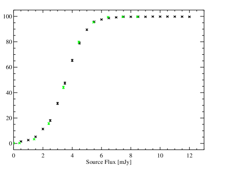
Figure 6: Survey completeness for the S/N$\geq$3.75 cut used here to select robust sources is represented with the dark symbols and error bars. The lighter symbols and error bars are estimates of the survey completeness when the integrated posterior flux distribution below 0 mJy is required to be $<$5%.

We next compute the survey completeness by injecting one source at a time, in the form of the point-source kernel scaled to represent each flux, at random positions in the GOODS-N signal map (Fig. 2) and tallying the instances when a new source is recovered with S/N$\geq$3.75 within 10 arcsec of the insertion point. We choose this radius because it is small enough for conducting quick searches in our simulations and because, barring incompleteness, simulations show that $>$99.5% of $\geq 3.75$-$\sigma$ sources will be found within 10 arcsec of their true position given the size of the AzTEC beam and the depth of coverage. This method of calculating completeness allows for the inclusion of “confusion noise” without altering the map properties appreciably, because only one artificial source is injected per simulation (Scott et al., 2006; Scott et al., 2008).

We have also assessed completeness by inserting point sources of known flux, one at a time, into pure noise-realisation maps rather than the signal map. With this method, we also require that each recovered artificial source has a $<5$% non-positive PFD. Since this constraint is essentially equivalent to a limiting S/N threshold of 3.75 (as evident from Table 1), it is not surprising that the survey completeness determined this way (lighter-shade points of Fig. 6) is similar to that derived from the previous method. The similarity in results also shows that the effects of confusion noise on survey completeness is small.

Finally, to verify that our source-candidate list has overlap with previously detected extragalactic (sub)mm sources, we compare our source list against 850-$\mu$m SCUBA detections within overlapping survey regions. For this purpose, we only consider the regions in the SCUBA/850-$\mu$m map with noise r.m.s. $<$ 2.5 mJy. Of the 28 AzTEC sources in the robust list, 11 lie within this region of the SCUBA map; of these 8 (73%) have robust detections at 850 $\mu$m (Pope et al., 2005) within 12 arcsec of the AzTEC position. Those 8 are highlighted with the superscript “$S$” in Table 1 while the other 3 are marked with the superscript “$N$.” On the other hand, all 38 robust SCUBA sources within the r.m.s. $<$ 2.5 mJy region (Pope et al., 2005; Wall et al., 2008) lie within the 70% coverage region of AzTEC. In Chapin et al. (in prep.) we will discuss the 850 $\mu$m properties of AzTEC sources by performing photometry in the SCUBA map at AzTEC positions, and more fully explore the overlap of the AzTEC and SCUBA populations in general.

5 1.1 mm Number counts

Using our AzTEC/GOODS-N data, we next quantify the number density of sources as a function of their intrinsic (de-boosted) 1.1 mm flux. These counts cannot be read directly from the recovered distribution of source flux densities due to: 1) the bias towards higher fluxes in the data (as described in section 4.2), which includes false detections; and 2) the survey incompleteness at lower fluxes. In order to estimate the counts we use two independent methods: a Monte Carlo technique that implicitly includes the flux bias and completeness issues; and a Bayesian approach that accounts for both these effects explicitly.

Fig. 7 shows the results of our number-counts simulations. It shows the source flux density histogram simulated for the best fit model from the parametric method overlaid on the actual distribution from the true map. It also shows the differential number counts vs. de-boosted source flux density as returned by both methods. The dot-dashed lines in the lower right correspond to the survey limits of the frequentist and Bayesian approaches, which are 27.8 and 33.8 deg^-2 mJy^-1, respectively. The survey limit is the y-axis value (number counts) that experiences Poisson deviations to zero sources per mJy-bin 32.7% of the time, given the map area considered. The two limits differ slightly because the frequentist simulations include the slightly larger area 50% coverage region, as opposed to the 70% coverage region that we use for the Bayesian method. The survey limit occurs at around 6 mJy for both the best-fit frequentist and Bayesian type simulations. Thus, we are not sensitive to the differential number counts with 1 mJy resolution beyond that point.

The power of the AzTEC/GOODS-N survey is in constraining number-counts at lower flux densities, given the depth reached in this relatively small field. We have, however, excluded results below the $<$2 mJy level from both methods, because of low survey completeness ($<$10%) and the possibility of increasing systematic effects. Therefore, the noteworthy features of Fig. 7 are the points from the Bayesian approach, indicated by crosses and error bars, in the range 2 mJy to 6 mJy and the allowed functional forms from the parametric (frequentist) method within those flux density bounds. Models allowed by the 68.3% confidence interval of the parametric method form the shaded region while the dark curve is the best-fit model. Given the error bounds from the two methods, they are in good agreement. Both methods are briefly described below.

5.1 Parametric frequentist approach

An obvious choice of indicator for the underlying source population is the recovered brightness distribution of source candidates in the GOODS-N map. Here, we use a S/N threshold of 3.5 and the 50% coverage region of the map. After identifying S/N$\geq$3.5 source candidates, we make a histogram of their measured flux densities using 0.25 mJy bins, for comparison against histograms made from simulating various number-counts models. This approach is similar, in spirit, to the method employed in Laurent et al. (2005) and the parametric version of number counts derived in Coppin et al. (2006). However, we avoid intermediate analytical constructs, as the procedure outlined below accounts for all relevant effects.

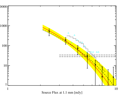
Figure 7: The thick solid curve and the enveloping shaded region correspond to the best fit number counts model and the 68.3% confidence interval from the parametric approach of § 5.1. The distribution of measured fluxes of 3.5-$\sigma$ sources in the actual map is shown by the triangles in the 3.5-8 mJy interval while the corresponding average distribution of the best fit model is indicated by the thin solid-line histogram. The difference between the thick solid line and the thin solid histogram indicates the importance of accounting for flux boosting and completeness. The crosses and error bars represent the differential number counts derived from the Bayesian method, which are in excellent agreement with the result from the parametric method. The dashed-line curve indicates the Bayesian prior. The upper and lower dot-dashed lines indicate the survey limits of the Bayesian and parametric methods, respectively.

We generate model realisation maps by injecting kernel-shaped point sources into noise realisation maps. The input source positions are uniformly distributed over the noise realisation map while their number density and flux distribution reflect the number-counts model being considered. For every model we have considered, we make 1200 simulated maps by constructing 12 different source realisations for each of the 100 noise realisation maps. Next, we use the same source-finding algorithm used on the signal map to extract all S/N$\geq$3.5 peaks in each simulated map. We then compare the average histogram of recovered source fluxes from the 1200 model realisations against the actual distribution of source fluxes. The data vs. models comparison is restricted to the 3.5–8 mJy measured flux density range. This comparison process is illustrated in Fig. 7.

The likelihood of the data given a model is determined according to Poisson statistics as in Laurent et al. (2005) and Coppin et al. (2006). One set of parameterised models that we have explored has the functional form given by Equation 1. We chose to re-parametrise these models so that the normalisation factor depends on only one of the fit parameters. The parameters we chose are the same $S^{\prime}$ as in Equation 1 and $N_{\rm 3mJy}$, the differential counts at 3 mJy, given by

$$N_{\rm 3mJy}=N^{\prime}\left({S^{\prime}\over 3\mathrm{mJy}}\right)e^{-3\mathrm{mJy}/S^{\prime}}.$$ (2)

In terms of these parameters, Equation 1 becomes

$${\mathrm{d}N\over\mathrm{d}S}=N_{\rm 3mJy}\left({3\mathrm{mJy}}\over S\right)e^{-(S-3\mathrm{mJy})/S^{\prime}}.$$ (3)

We explored the $S^{\prime}$–$N_{\rm 3mJy}$ parameter space over the rectangular region bracketed by 0.5-2 mJy and 60-960 mJy^-1 degree^-2 using a $(\Delta S^{\prime},\Delta N_{\rm 3mJy})$ cell size of (0.15,60). The likelihood function, ${\cal L}$, is a maximum for the model with $S^{\prime}=1.25\pm 0.38\,$mJy and $N_{\rm 3mJy}=300\pm 90$ mJy^-1 degree^-2. We did not assume $\chi^{2}$-like behaviour of $-\ln({\cal L})$ for calculating the 68.3% confidence contours whose projections are the error bars quoted above. Instead, as outlined in Press et al. (1992), we made many realisations of the best-fit model and put them through the same parameter estimation procedure that was applied to the actual data. In terms of the goodness of fit, we find that 66% of the simulated fits yield a higher value of $-\ln({\cal L})$ compared to the actual value. Fig. 7 shows this best-fit number-counts estimate against the de-boosted 1.1 mm flux density along with a continuum of curves allowed by the 68.3% confidence region.

5.2 Bayesian method

We also estimate number counts from the individual source PFDs calculated in § 4.2 using a modified version of the bootstrapping method described in Coppin et al. (2006). A complete discussion of the modifications and tests of the method will be presented in Austermann et al. (in prep.). For these calculations, we use only the sub-list of robust sources in Table 1. We have repeated this bootstrapping process 20,000 times to measure the mean and uncertainty distributions of source counts in this field. The differential and integrated number counts extracted with this method, using $1\,$mJy bins, are shown in Fig. 7. Our simulations show that the extracted number counts are quite reliable for a wide range of source populations and only weakly dependent on the assumed population used to generate the Bayesian prior (the dashed-line curve of Fig. 7) with the exception of the lowest flux density bins, below 2 mJy, which suffer from source confusion and low (and poorly constrained) completeness. Overall, the results from the Bayesian method are in excellent agreement with those from the parametric method between the lower sensitivity bound (2 mJy) and the survey limit ($\sim$6 mJy).

6 Discussion

Figure 8: The cumulative (integral) number counts from other 1.1–1.2 mm surveys are shown alongside our results. The AzTEC/GOODS-N parametric number-counts results are indicated by the hatched region that represents the 68.3% confidence region for parametric models. The dot-dashed line indicates the survey limit. Results from the Bolocam 1.1 mm Lockman Hole survey are indicated by a thin solid line and two bounding dotted-lines that represent the best-fit model and 68.3% confidence region as found by Maloney et al. (2005). The 1.2-mm MAMBO-IRAM results reported in Greve et al. (2004) also shown (triangles). The stars represent the “reduction D” results of Coppin et al. (2006) with 850 $\mu$m flux densities scaled by the factor 1/2.08 as explained in the text. The dashed curve indicates the best combined fit to the Bayesian results from both surveys.

In Fig. 8, we display our cumulative number-counts results with the 68.3%-allowed hatched region derived from the parametric method. We next compare those results with previous surveys of (sub)mm galaxies. Combined results from the 1.2-mm MAMBO surveys of the Lockman Hole and ELAIS-N2 region (Greve et al., 2004) and the 1.1-mm Bolocam Lockman Hole survey (Maloney et al., 2005) are shown in Fig. 8. Our GOODS-N number counts are in good agreement with MAMBO results. Our results are in disagreement with the results of Maloney et al. (2005), even within a limited flux range such as 3–6 mJy where we expect both surveys to be sensitive to the number counts.

In Fig. 8, we also compare our results with the 850-$\mu$m number counts of Coppin et al. (2006). If the 1.1–1.2 mm surveys detect the same population of sub-mm sources seen by SCUBA at 850$\,\mu$m – an assumption that is not obviously valid given the possible redshift-dependent selection effects (Blain et al., 2002) – we would expect a general correspondence between number counts at these two wavelengths, with a scaling in flux density that represents the spectral factor for an average source. Therefore, we perform a simultaneous fit to the SCUBA/SHADES and AzTEC/GOODS-N differential Bayesian number counts in order to determine the average dust emissivity spectral index, $\alpha_{\rm{dust}}$ (and thus the flux density scaling factor from 1.1 mm wavelength to 850 $\mu$m wavelength), and the parameters, $N_{\rm 3mJy}$ and $S^{\prime}$, of Equation 3. This fit results in the best-fit parameters and correlation matrix given in Table 3. We overlay the Coppin et al. (2006) number counts on Fig. 8 with the 850-$\mu$m fluxes scaled by the scaling factor derived from this fit, which is 2.08$\pm$0.18. For visual comparison, the shaded region of Fig. 8, which represents our parametric result, is sufficient because it represents well the results from both methods (see Fig. 7). Fig. 8 shows that the scaled SCUBA-SHADES points fall well within the bounds allowed by our results.

Survey	$S^{\prime}$	$N_{\rm 3mJy}$	$\alpha_{\rm{dust}}$
AzTEC/GOODS-N	$1.25\pm 0.38$	$300\pm 90$
AzTEC/GOODS-N
+ SCUBA/SHADES	$1.60\pm 0.25$	$274\pm 54$	$2.84\pm 0.32$
	$S^{\prime}$	$N_{\rm 3mJy}$	$\alpha_{\rm{dust}}$
$S^{\prime}$	1	0.05	-0.32
$N_{\rm 3mJy}$	0.05	1	-0.8
$\alpha_{\rm{dust}}$	-0.32	-0.8	1

Table 3: Best-fit Schechter function parameters and dust emissivity spectral index using the Bayesian results from the AzTEC/GOODS-N, SCUBA/SHADES, and combined surveys. The correlation matrix for the combined fit is also listed. Caveats on this analysis are given in the text.

The $\alpha_{\rm{dust}}$ of Table 3 was computed for the nominal AzTEC and SCUBA band centres, which are 1.1 mm and 850 $\mu$m respectively. However, the quoted error on $\alpha_{\rm{dust}}$ brackets the effects of small shifts in the effective band centres due to spectral index differences between SMGs and flux calibrators. The dust emissivity spectral index may also be estimated by averaging the 1.1 mm to 850 $\mu$m flux density ratio of individual sources or by performing the appropriate stacking analysis. Due to the moderate S/N of sources in our surveys, the effects of flux bias and survey completeness must be accounted for in such analyses. Therefore, performing a combined fit to the differential number counts vs. de-boosted flux from the two surveys, where those effects are already included, is an appropriate method for estimating the spectral index. From Fig. 8, the hypothesis that SCUBA and AzTEC detect the same underlying source population appears plausible.

However, we do not comment on the formal goodness of fit as the $\chi^{2}$ obtained for the combined fit is unreasonably small because the full degree of correlation between data points is underestimated in the standard computation of the two covariance matrices (Coppin et al., 2006). In addition, the best-fit parameters of the combined fit may have a large scatter from a global mean value (if one exists), due to sample variance, as the two surveys cover different fields. Although SCUBA 850 $\mu$m number-counts are available for GOODS-N (Borys et al., 2003), the survey region (see Fig. 1) and the method used to estimate number counts in that work are quite different from those used here. Therefore, we chose to fit to the SCUBA/SHADES number counts (Coppin et al., 2006) instead, since they were determined using methods similar to ours.

7 Conclusion

We have used the AzTEC instrument on the JCMT to image the GOODS-N field at 1.1 mm. The map has nearly uniform noise of 0.96–1.16$\,{\rm mJy}\,{\rm beam}^{-1}$ across a field of $245\,{\rm arcmin}^{2}$. A stacking analysis of the map flux at known radio source locations shows that any systematic pointing error for the map is smaller than 1 arcsec in both RA and Dec. Thus, the dominant astrometric errors for the 36 source-candidates with S/N$\geq$3.5 are due to noise in the centroid determination for each source. Using a S/N$\geq$3.75 threshold for source robustness, we identify a subset of 28 source candidates among which we only expect 1–2 noise-induced spurious detections. Furthermore, of the 11 AzTEC sources that fall within the considered region of the SCUBA/850-$\mu$m, 8 are detected unambiguously.

This AzTEC map of GOODS-N represents one of the largest, deepest mm-wavelength surveys taken to date and provides new constraints on the number counts at the faint end (down to ${\sim}\,2\,{\rm mJy}$) of the 1.1 mm galaxy population. We compare two very different techniques to estimate the number density of sources as a function of their intrinsic flux–a frequentist technique based on the flux histogram of detected sources in the map similar in spirit to that of Laurent et al. (2005), and a Bayesian approach similar to that of Coppin et al. (2006). Reassuringly, the two techniques give similar estimates for the number counts. Those results are in good agreement with the number counts estimates of Greve et al. (2004) but differ significantly from those of Maloney et al. (2005).

The 1.1 mm number counts from this field are consistent with a direct flux scaling of the 850 µm SCUBA/SHADES number counts (Coppin et al., 2006) within the uncertainty of the two measurements, with a flux density scaling factor of $2.08\pm 0.18$. If we assume that the two instruments are detecting the same population of sources, we obtain a grey body emissivity index of $2.84\pm 0.32$ for the dust in the sources. While there is no evidence based on the number counts that 1.1 mm surveys select a significantly different population than 850 µm surveys, we caution that the number counts alone cannot really test this hypothesis. A more thorough study of whether AzTEC is selecting a systematically different population than SCUBA can come only from comparison of the redshifts and multi-wavelength SEDs of the identified galaxies, which we will describe in Chapin et al. (in prep.), the second paper in this series.

There is also a survey of GOODS-N with MAMBO at 1.25 mm performed by Greve et al. (in prep.). A comparison between these two millimetre maps and, possibly, the SCUBA ‘Super-map’ is reserved for a future paper (Pope et al. in prep.).

This AzTEC/GOODS-N map is one of the large blank-field SMG surveys at 1.1 mm taken at the JCMT. Combined with the AzTEC surveys in the COSMOS (Scott et al., 2008) and SHADES (Austermann et al. in prep.) fields, these GOODS-N data will allow a study of clustering and cosmic variance on larger spatial scales than any existing (sub)mm extragalactic surveys.

References

- Alexander et al. (2003) Alexander D. M., et al., 2003, AJ, 126, 539
- Barger et al. (2000) Barger A. J., Cowie L. L., Richards E. A., 2000, AJ, 119, 2092
- Barger et al. (1999) Barger A. J., Cowie L. L., Sanders D. B., 1999, ApJ, 518, L5
- Barger et al. (1998) Barger A. J., Cowie L. L., Sanders D. B., Fulton E., Taniguchi Y., Sato Y., Kawara K., Okuda H., 1998, Nature, 394, 248
- Bertoldi et al. (2007) Bertoldi F., et al., 2007, ApJS, 172, 132
- Blain et al. (1999) Blain A. W., Kneib J.-P., Ivison R. J., Smail I., 1999, ApJ, 512, L87
- Blain et al. (2002) Blain A. W., Smail I., Ivison R. J., Kneib J.-P., Frayer D. T., 2002, Phys. Rep., 369, 111
- Borne et al. (2000) Borne K. D., Bushouse H., Lucas R. A., Colina L., 2000, ApJ, 529, L77
- Borys et al. (2003) Borys C., Chapman S., Halpern M., Scott D., 2003, MNRAS, 344, 385
- Coppin et al. (2006) Coppin K., et al., 2006, MNRAS, 372, 1621
- Coppin et al. (2005) Coppin K., Halpern M., Scott D., Borys C., Chapman S., 2005, MNRAS, 357, 1022
- Coppin et al. (2008) Coppin K., Halpern M., Scott D., Borys C., Dunlop J., Dunne L., Ivison R., Wagg J., et al., 2008, MNRAS, 384, 1597
- Cowie et al. (2004) Cowie L. L., Barger A. J., Hu E. M., Capak P., Songaila A., 2004, AJ, 127, 3137
- Cowie et al. (2002) Cowie L. L., Barger A. J., Kneib J.-P., 2002, AJ, 123, 2197
- Dunlop et al. (1994) Dunlop J. S., Hughes D. H., Rawlings S., Eales S. A., Ward M. J., 1994, Nature, 370, 347
- Eales et al. (2000) Eales S., Lilly S., Webb T., Dunne L., Gear W., Clements D., Yun M., 2000, AJ, 120, 2244
- Giavalisco et al. (2004) Giavalisco M., et al., 2004, ApJ, 600, L93
- Greve et al. (2004) Greve T. R., Ivison R. J., Bertoldi F., Stevens J. A., Dunlop J. S., Lutz D., Carilli C. L., 2004, Monthly Notices of the RAS, 354, 779
- Hughes et al. (1998) Hughes D. H., Serjeant S., Dunlop J., Rowan-Robinson M., Blain A., Mann R. G., Ivison R., Peacock J., Efstathiou A., Gear W., Oliver S., Lawrence A., Longair M., Goldschmidt P., Jenness T., 1998, Nature, 394, 241
- Ivison et al. (2007) Ivison R. J., et al., 2007, MNRAS, 380, 199
- Kovács et al. (2006) Kovács A., Chapman S. C., Dowell C. D., Blain A. W., Ivison R. J., Smail I., Phillips T. G., 2006, ApJ, 650, 592
- Laurent et al. (2005) Laurent G. T., et al., 2005, Astrophysical Journal, 623, 742
- Maloney et al. (2005) Maloney P. R., Glenn J., Aguirre J. E., Golwala S. R., Laurent G. T., Ade P. A. R., Bock J. J., Edgington S. F., Goldin A., Haig D., Lange A. E., Mauskopf P. D., Nguyen H., Rossinot P., Sayers J., Stover P., 2005, ApJ, 635, 1044
- Pope et al. (2005) Pope A., Borys C., Scott D., Conselice C., Dickinson M., Mobasher B., 2005, MNRAS, 358, 149
- Pope et al. (2006) Pope A., Scott D., Dickinson M., Chary R.-R., Morrison G., Borys C., Sajina A., Alexander D. M., Daddi E., Frayer D., MacDonald E., Stern D., 2006, MNRAS, 370, 1185
- Press et al. (1992) Press W. H., Teukolsky S. A., Vetterling W. T., Flannery B. P., 1992, Numerical Recipes in C: The Art of Scientific Computing, 2nd edn. Cambridge Univ., Cambridge
- Richards (2000) Richards E. A., 2000, ApJ, 533, 611
- Scott et al. (2008) Scott K. S., et al., 2008, accepted to MNRAS, arXiv:astro-ph/0801.2779
- Scott et al. (2006) Scott S. E., Dunlop J. S., Serjeant S., 2006, MNRAS, 370, 1057
- Scott et al. (2002) Scott S. E., Fox M. J., Dunlop J. S., Serjeant S., Peacock J. A., Ivison R. J., Oliver S., Mann R. G., Lawrence A., Efstathiou A., Rowan-Robinson M., Hughes D. H., Archibald E. N., Blain A., Longair M., 2002, MNRAS, 331, 817
- Smail et al. (1997) Smail I., Ivison R. J., Blain A. W., 1997, ApJ, 490, L5+
- Wall et al. (2008) Wall J. V., Pope A., Scott D., 2008, MNRAS, 383, 435
- Wang et al. (2004) Wang W.-H., Cowie L. L., Barger A. J., 2004, ApJ, 613, 655
- Webb et al. (2003) Webb T. M., Eales S. A., Lilly S. J., Clements D. L., Dunne L., Gear W. K., Ivison R. J., Flores H., Yun M., 2003, ApJ, 587, 41
- Wilson et al. (2008) Wilson G. W., et al., 2008, accepted to MNRAS, arXiv:astro-ph/0801.2783
- Wirth et al. (2004) Wirth G. D., Willmer C. N. A., Amico P., Chaffee F. H., Goodrich R. W., Kwok S., Lyke J. E., Mader J. A., et al., 2004, AJ, 127, 3121