Ricci-flat Kähler metrics on crepant resolutions of Kähler cones

Abstract.

We prove that a crepant resolution $\pi:Y\rightarrow X$ of a Ricci-flat Kähler cone $X$ admits a complete Ricci-flat Kähler metric asymptotic to the cone metric in every Kähler class in $H^{2}_{c}(Y,\mathbb{R})$. A Kähler cone $(X,\bar{g})$ is a metric cone over a Sasaki manifold $(S,g)$, i.e. $X=C(S):=S\times\mathbb{R}_{>0}$ with $\bar{g}=dr^{2}+r^{2}g$, and $(X,\bar{g})$ is Ricci-flat precisely when $(S,g)$ Einstein of positive scalar curvature. This result contains as a subset the existence of ALE Ricci-flat Kähler metrics on crepant resolutions $\pi:Y\rightarrow X=\mathbb{C}^{n}/\Gamma$, with $\Gamma\subset SL(n,\mathbb{C})$, due to P. Kronheimer $(n=2)$ and D. Joyce $(n>2)$.

We then consider the case when $X=C(S)$ is toric. It is a result of A. Futaki, H. Ono, and G. Wang that any Gorenstein toric Kähler cone admits a Ricci-flat Kähler cone metric. It follows that if a toric Kähler cone $X=C(S)$ admits a crepant resolution $\pi:Y\rightarrow X$, then $Y$ admits a $T^{n}$-invariant Ricci-flat Kähler metric asymptotic to the cone metric $(X,\bar{g})$ in every Kähler class in $H^{2}_{c}(Y,\mathbb{R})$. A crepant resolution, in this context, is a simplicial fan refining the convex polyhedral cone defining $X$. We then list some examples which are easy to construct using toric geometry.

1. Introduction

There has been much research recently in constructing examples of Sasaki-Einstein manifolds (cf. [7, 5, 28, 17, 16, 15]). Recall that a Sasaki-Einstein manifold $(S,g)$ is positive scalar curvature Einstein manifold whose metric cone $(C(S),\bar{g})$, $C(S)=\mathbb{R}_{>0}\times S$ and $\bar{g}=dr^{2}+r^{2}g$, is Ricci-flat Kähler. In all cases besides $S=S^{2n-1}$, $C(S)=\mathbb{C}^{n}$, the cone has a singularity at the apex. There has been interest recently in constructing Ricci-flat Kähler metrics on resolutions $\pi:Y\rightarrow X$ of the singularity of $X$. One source of interest in these asymptotically conical Calabi-Yau manifolds is in the AdS/CFT correspondence (cf. [30, 31]). Another motivation is in the construction of new Calabi-Yau manifolds by resolving conical singularities of a singular Calabi-Yau space (cf [11, 12]).

The resolution will necessarily be crepant, and one requires that the metric on $Y$ be asymptotic to the original Ricci-flat Kähler cone metric on $X$. In this article we will give a partial solution to the existence of such metrics. Many examples are already known. In particular, when $C(S)=\mathbb{C}^{n}/\Gamma$, for $\Gamma\subset SL(n,\mathbb{C})$ a finite group acting freely on $\mathbb{C}^{n}\setminus\{o\}$, such a metric on a resolution of $X$ will be an ALE Ricci-flat Kähler metric. The existence and uniqueness of ALE Ricci-flat Kähler metrics, in each Kähler class, on $X$ has been proved by P. Kronheimer [25] for $n=2$ and by D. Joyce [23, 22] for $n>2$.

Until recently all known examples of Sasaki-Einstein manifolds were quasi-regular, meaning they are orbifold fibrations over Kähler Einstein orbifolds. The 5-dimensional Sasaki-Einstein manifolds $Y^{p,q}$ of J. Gauntlett, D. Martelli, J. Sparks, and D. Waldram [17] provided the first irregular examples, meaning that they are not simply orbifold fibrations over a Kähler-Einstein orbifold. The general existence problem for Sasaki-Einstein metrics on toric Sasaki manifolds has been solved in general in the beautiful paper of A. Futaki, H. Ono, G. Wang [15]. In other words, their result implies that any toric $\mathbb{Q}$-Gorenstein isolated singularity $X$ admits a Ricci-flat Kähler cone metric. This will be used as a source of examples in this article. Although a crepant resolution does not always exist, it is elementary to construct examples using toric geometry.

Previous constructions of complete Ricci-flat Kähler metrics such as those of G. Tian and S.-T. Yau [37, 38] constructed metrics asymptotic, in some sense, to a cone over a regular, or quasi-regular, Sasaki-Einstein manifold. The present work differs in that the existence of complete Ricci-flat metrics are proved which are asymptotic to cones over irregular Sasaki-Einstein manifolds. Some explicit examples of Ricci-flat Kähler metrics asymptotic to cones over irregular Sasaki-Einstein manifolds were constructed in [29]. The author has also considered the possibility of such metrics on quasi-projective manifolds in [40], which is very complementary to this article.

This article considers the following conjecture which first appeared in [31].

Conjecture 1.1.

Let $\pi:Y\rightarrow X$ be a crepant resolution of an isolated singularity $X=C(S)$, where $C(S)$ admits a Ricci-flat Kähler cone metric. Then $Y$ admits a unique Ricci-flat Kähler metric in each Kähler class in $H^{2}(Y,\mathbb{R})$ that is asymptotic to a cone over the Sasaki-Einstein manifold $(S,g)$.

We give a partial solution to this conjecture. We prove the following, where $H_{c}^{2}(Y,\mathbb{R})$ denotes cohomology with compact supports.

Theorem 1.2.

Let $\pi:Y\rightarrow X$ be a crepant resolution of the isolated singularity of $X=C(S)$, where $C(S)$ admits a Ricci-flat Kähler cone metric. Then $Y$ admits a Ricci-flat Kähler metric $g$ in each Kähler class in $H_{c}^{2}(Y,\mathbb{R})\subset H^{2}(Y,\mathbb{R})$ which is asymptotic to the Kähler cone metric $\bar{g}$ on $X$ as follows. There is an $R>0$ such that, for any $\delta>0$ and $k\geq 0$,

(1) $$\nabla^{k}\left(\pi_{*}g-\bar{g}\right)=O\left(r^{-2n+\delta-k}\right)\quad\text{on }\{y\in C(S):r(y)>R\},$$

where $\nabla$ is the covariant derivative of $\bar{g}$.

Note that the inclusion of compactly supported cohomology in this case induces an inclusion $H_{c}^{2}(Y,\mathbb{R})\subset H^{2}(Y,\mathbb{R})$. And $H_{c}^{2}(Y,\mathbb{R})$ is the subset of $H^{2}(Y,\mathbb{R})$ whose restriction to $S\subset X$ vanishes. Also, if $\omega$ is a Kähler class in $H_{c}^{2}(Y,\mathbb{R})$, then it has a d-dimensional neighborhood of Kähler classes, where $d=\dim H_{c}^{2}(Y,\mathbb{R})$. Thus the theorem gives families of Ricci-flat metrics. Note also that $d$ is the number of prime divisors in the exceptional set $E=\pi^{-1}(o)$.

It is also useful to consider partial crepant resolutions $\pi:Y\rightarrow X$ where $Y$ has only orbifold singularities. The proof of Theorem 1.2 is valid without modification in this case also. Many of the examples of Sasaki-Einstein manifolds $S$ have associated Ricci-flat Kähler cones $X=C(S)$ which do not admit crepant resolutions, but nonetheless admit such a partial crepant resolution. This is true of some of the examples constructed via hypersurface singularities in [5] and [7], while some examples do admit crepant resolutions.

Theorem 1.2 solves a large portion of Conjecture 1.1. But it is instructive to consider what it excludes. If $\pi:Y\rightarrow X$ is a small resolution, i.e. $\operatorname{codim}_{\mathbb{C}}(E)>1$, where $E=\pi^{-1}(o)$ is the exceptional set, then there are no Kähler classes in $H_{c}^{2}(Y,\mathbb{R})$. In particular, consider the conifold $X=\{z_{0}^{2}+z_{1}^{2}+z_{2}^{2}+z_{3}^{2}=0\}\subset\mathbb{C}^{4}$ which is the cone over $S^{2}\times S^{3}$. It has the structure of a Ricci-flat Kähler cone if $S^{2}\times S^{3}$ is given the homogeneous Sasaki-Einstein metric. Then $X$ admits a crepant resolution $\pi:Y\rightarrow X$, where $Y$ is the total space of $\mathcal{O}(-1)\oplus\mathcal{O}(-1)\rightarrow\mathbb{C}P^{1}$. The exceptional set is $\mathbb{C}P^{1}=\pi^{-1}(o)$. Nevertheless, it is well known that $Y$ admits a complete Ricci-flat Kähler metric (cf. [11]).

After proving Theorem 1.2 we will consider the toric case in more detail. In this case $X=C(S)$ is a Gorenstein toric Kähler cone which admits a toric Ricci-flat Kähler cone metric by the results of [15]. In this case a crepant resolution $\pi:Y\rightarrow X$ is toric, and $Y$ is described explicitly by a nonsingular simplicial fan $\tilde{\Delta}$ refining the convex polyhedral cone $\Delta$ defining $X$. A Kähler class in $H_{c}^{2}(Y,\mathbb{R})$ is characterized by a compact strictly convex support function on $\tilde{\Delta}$. This is a strictly convex support function on $\tilde{\Delta}$ which vanishes on the rays defining $\Delta$. We prove the following.

Corollary 1.3.

Let $\pi:Y\rightarrow X$ be a crepant resolution of a Gorenstein toric Kähler cone $X$. Suppose the fan $\tilde{\Delta}$ defining $Y$ admits a compact strictly convex support function. Then $Y$ admits a Ricci-flat Kähler metric $g$ which is asymptotic to $(C(S),\bar{g})$ as in (1). Furthermore, $g$ is invariant under the compact $n$-torus $T^{n}$.

As above, if a Ricci-flat Kähler metric exists, then there is a d-dimensional, $d=\dim H_{c}^{2}(Y,\mathbb{R})$, family of such metrics. Here $d$ is the number of lattice points in the interior of a polytope $P_{\Delta}$ which is the intersection of the cone $\Delta$ defining $X$ with a hyperplane. Thus, although crepant resolutions are generally not unique, $d$ is invariant. A crepant resolution of $X$ is characterized by a basic lattice triangulation of $P_{\Delta}$. When $n=3$ such a triangulation always exists.

In the final section we give some examples. These are easily described by the toric geometry of the resolution $\pi:Y\rightarrow X$ in the toric case. Many more examples are constructed in [39] using toric geometry and by resolving hypersurface singularities. Recently the author has come up with a proof which removes the $\delta>0$ from the convergence in (1) and thus gives the sharp convergence. This will appear in a subsequent article.

2. Sasaki manifolds

We review some of the properties of Sasaki manifolds. We are primarily interested in Kähler cones. But a Kähler cone is a cone over a Sasaki manifold, and much research has been done recently on Sasaki-Einstein manifolds (cf. [3, 6]).

Definition 2.1.

A Riemannian manifold $(S,g)$ of dimension $2n-1$ is Sasakian if the metric cone $(C(S),\bar{g})$, $C(S)=\mathbb{R}_{>0}\times S$ and $\bar{g}=dr^{2}+r^{2}g$, is Kähler.

Set $\tilde{\xi}=J(r\frac{\partial}{\partial r})$, then $\tilde{\xi}-iJ\tilde{\xi}$ is a holomorphic vector field on $C(S)$. The restriction $\xi$ of $\tilde{\xi}$ to $S=\{r=1\}\subset C(S)$ is the Reeb vector field of $S$, which is a Killing vector field. If the orbits of $\xi$ close, then it defines a locally free $U(1)$-action on $S$. If the $U(1)$-action is free, then the Sasaki structure is said to be regular. If there are non-trivial stablizers then the Sasaki structure is quasi-regular. If the orbits do not close the Sasaki structure is irregular.

Let $\eta$ be the dual 1-form to $\xi$ with respect to $g$. Then

(2) $$\eta=(2d^{c}\log r)|_{r=1},$$

where $d^{c}=\frac{i}{2}(\bar{\partial}-\partial)$. Let $D=\ker\eta$. Then $d\eta$ in non-degenerate on $D$ and $\eta$ is a contact form on $S$. Furthermore, we have

(3) $$d\eta(X,Y)=2g(\Phi X,Y),\quad\text{for }X,Y\in D_{x},x\in S,$$

where $\Phi|_{D_{x}}$ is the restriction of the complex structure $J$ on $C(S)$, to $D_{x}$, and $\Phi(\xi)=0$. Thus $(D,J)$ is a strictly pseudo-convex CR structure on $S$. We will denote the Sasaki structure on $S$ by $(g,\xi,\eta,\Phi)$. It follows from (2) that the Kähler form of $(C(S),\bar{g})$ is

(4) $$\omega=\frac{1}{2}d(r^{2}\eta)=\frac{1}{2}dd^{c}r^{2}.$$

Thus $\frac{1}{2}r^{2}$ is a Kähler potential for $\omega$.

There is a 1-dimensional foliation $\mathscr{F}_{\xi}$ generated by the Reeb vector field $\xi$. Since the leaf space is identical with that generated by $\tilde{\xi}-iJ\tilde{\xi}$ on $C(S)$, $\mathscr{F}_{\xi}$ has a natural transverse holomorphic structure. And $\omega^{T}=\frac{1}{2}d\eta$ defines a Kähler form on the leaf space. We denote the transverse Kähler metric by $g^{T}$. Note that when the Sasaki structure on $S$ is regular (resp. quasi-regular), the leaf space of $\mathscr{F}_{\xi}$ is a Kähler manifold (resp. orbifold).

A p-form $\alpha\in\Omega^{p}(S)$ on $S$ is said to be basic if

(5) $$\xi\,\lrcorner\,\alpha=0\quad\text{and}\quad\mathcal{L}_{\xi}\alpha=0.$$

The basic p-forms are denoted by $\Omega_{B}^{p}(S)$, where the foliation $\mathscr{F}_{\xi}$ on $S$ must be fixed. One easily checks that $\Omega_{B}^{*}$ is closed under the exterior derivative. So there is a transversal de Rham complex which can be used to calculate the basic cohomology $H^{*}_{B}(S)$.

The foliation $\mathscr{F}_{\xi}$ associated to a Sasaki structure has a transverse holomorphic structure, so there is a splitting $\Omega_{B}^{k}=\bigoplus_{p+q=k}\Omega_{B}^{p,q}$ of complex forms into types. And the exterior derivative on basic forms splits into $d=\partial+\bar{\partial}$, where $\partial$ has degree $(1,0)$ and $\bar{\partial}$ has degree $(0,1)$. Thus we have as well the basic Dolbeault complex and the basic Dolbeault cohomology groups $H^{p,q}_{B}(S)$.

Furthermore, the foliation has a transverse Kähler structure, and the usual Hodge theory for Kähler manifolds carries over. In particular, we have the Hodge decomposition $H^{k}_{B}(S,\mathbb{C})=\bigoplus_{p+q=k}H^{p,q}_{B}(S)$ and the representation of basic cohomology classes by harmonic forms. It is also useful to know that the $\partial\bar{\partial}$-lemma holds for basic forms as it does on Kähler manifolds. Thus if $\phi\in\Omega^{1,1}_{B}$ is exact, then there is a basic $f\in C_{B}^{\infty}$ with $\phi=i\partial\bar{\partial}f$ and $f$ can be taken to be real if $\phi$ is. See the monograph [6] for a survey of these results.

We will consider deformations of the transverse Kähler structure. Let $\phi\in C^{\infty}_{B}(S)$ be a smooth basic function. Then set

(6) $$\tilde{\eta}=\eta+2d^{c}_{B}\phi.$$

Then

$$d\tilde{\eta}=d\eta+2d_{B}d^{c}_{B}\phi=d\eta+2i\partial_{B}\bar{\partial}_{B}\phi.$$

For sufficiently small $\phi$, $\tilde{\eta}$ is a non-degenerate contact form in that $\tilde{\eta}\wedge d\tilde{\eta}^{n}$ is nowhere zero. Then we have a new Sasaki structure on $S$ with the same Reeb vector field $\xi$, transverse holomorphic structure on $\mathscr{F}_{\xi}$, and holomorphic structure on $C(S)$. This Sasaki structure has transverse Kähler form $\tilde{\omega}^{T}=\omega^{T}+i\partial_{B}\bar{\partial}_{B}\phi$. One can show [15] that if

$$\tilde{r}=r\exp{\phi},$$

then $\tilde{\omega}=\frac{1}{2}dd^{c}\tilde{r}^{2}$ is the Kähler form on $C(S)$ associated to the transversally deformed Sasaki structure.

Proposition 2.2.

Let $(S,g)$ be a $2n-1$-dimensional Sasaki manifold. Then the following are equivalent.

• $(S,g)$ is Sasaki-Einstein with the Einstein constant being necessarily $2n-2$.

• $(C(S),\bar{g})$ is a Ricci-flat Kähler.

• The Kähler structure on the leaf space of $\mathscr{F}_{\xi}$ is Kähler-Einstein with Einstein constant $2n$.

This follows from elementary computations. In particular, the equivalence of (i) and (iii) follows from

(7) $$\operatorname{Ric}_{g}(\tilde{X},\tilde{Y})=(\operatorname{Ric}^{T}-2g^{T})(X,Y),$$

where $\tilde{X},\tilde{Y}\in D$ are lifts of $X,Y$ in the local leaf space; $g^{T}$ and $\operatorname{Ric}^{T}$ are the metric and Ricci tensor of the transversal Kähler structure.

Given a Sasaki structure we can perform a $D$-homothetic transformation to get a new Sasaki structure. For $a>0$ set

(8) $$\eta^{\prime}=a\eta,\quad\xi^{\prime}=\frac{1}{a}\xi,$$

(9) $$g^{\prime}=ag^{T}+a^{2}\eta\otimes\eta=ag+(a^{2}-a)\eta\otimes\eta.$$

Then $(g^{\prime},\xi^{\prime},\eta^{\prime},\Phi)$ is a Sasaki structure with the same holomorphic structure on $C(S)$, and with $r^{\prime}=r^{a}$.

Proposition 2.3.

The following necessary conditions for $S$ to admit a deformation of the transverse Kähler structure to a Sasaki-Einstein metric are equivalent.

• $c_{1}^{B}=a[d\eta]$ for some positive constant $a$.

• $c_{1}^{B}>0$, i.e. represented by a positive $(1,1)$-form, and $c_{1}(D)=0$.

• For some positive integer $\ell>0$, the $\ell$-th power of the canonical line bundle $\mathbf{K}^{\ell}_{C(S)}$ admits a nowhere vanishing section $\Omega$ with $\mathcal{L}_{\xi}\Omega=in\Omega$.

Proof.

Let $\rho$ denote the Ricci form of $(C(S),\bar{g})$ and $\rho^{T}$ the Ricci form of $\operatorname{Ric}^{T}$, then easy computation shows that

(11) $$\rho=\rho^{T}-2n\frac{1}{2}d\eta.$$

If (i) is satisfied, there is a $D$-homothety so that $[\rho^{T}]=2n[\frac{1}{2}d\eta]$ as basic classes. Thus there exists a smooth function $h$ with $\xi h=0=r\frac{\partial}{\partial r}h$ and

(12) $$\rho=i\partial\bar{\partial}h.$$

This implies that $e^{h}\frac{\omega^{n}}{n!}$, where $\omega$ is the Kähler form of $\bar{g}$, defines a flat metric $|\cdot|$ on $\mathbf{K}_{C(S)}$. Parallel translation defines a multi-valued section which defines a holomorphic section $\Omega$ of $\mathbf{K}^{\ell}_{C(S)}$ for some integer $\ell>0$ with $|\Omega|=1$. Then we have

(13) $$\left(\frac{i}{2}\right)^{n}(-1)^{\frac{n(n-1)}{2}}\Omega\wedge\bar{\Omega}=e^{h}\frac{1}{n!}\omega^{n}.$$

From the invariance of $h$ and the fact that $\omega$ is homogeneous of degree 2, we see that $\mathcal{L}_{r\frac{\partial}{\partial r}}\Omega=n\Omega$.

Conversely, if (iii) holds, then we have (13) for some $h\in C^{\infty}(C(S))$. Then since $\omega$ is homogeneous of degree 2 and $\mathcal{L}_{r\frac{\partial}{\partial r}}\Omega=n\Omega$, it follows that $\xi h=0=r\frac{\partial}{\partial r}h$. And the above arguments show that $c_{1}^{B}=\frac{1}{2\pi}[\rho^{T}]=\frac{n}{\pi}[d\eta]$.

The equivalence of (i) and (ii) is easy (cf. [15] Proposition 4.3). ∎

Example 2.4 Let $Z$ be a complex manifold (or orbifold) with a negative holomorphic line bundle (respectively V-bundle) $\mathbf{L}$. If the total space of $\mathbf{L}^{\times}$, $\mathbf{L}$ minus the zero section, is smooth, then the $U(1)$-subbundle $S\subset\mathbf{L}^{\times}$ has a natural regular (respectively quasi-regular) Sasaki structure. Let $h$ be an Hermitian metric on $\mathbf{L}$ with negative curvature. If in local holomorphic coordinates we define $r^{2}=h|z|^{2}$, where $z$ is the fiber coordinate, then $\omega=\frac{1}{2}dd^{c}r^{2}$ is the Kähler form on $\mathbf{L}^{\times}$ of a Kähler cone metric. And $S=\{z\in\mathbf{L}^{\times}:r(z)=1\}$ has the induced Sasaki structure. Conversely, it can be shown that every regular (respectively quasi-regular) Sasaki structure arises from this construction (cf. [3]). $\diamondsuit$

3. Crepant resolutions

Let $C(S)$ be a Kähler cone. Note that a priori $C(S)$ does not contain the vertex, but $X=C(S)\cup\{o\}$ can be made into a complex space in a unique way. The Reeb vector field $\xi$ generates a 1-parameter subgroup of the automorphism group $\operatorname{Aut}(S)$ of the Sasaki manifold $S$. Since $\operatorname{Aut}(S)$ is compact, the closure of this subgroup is a torus $T^{k}\subset\operatorname{Aut}(S)$. Here $\operatorname{rank}(S):=k$. Choose a vector field $\zeta$ in the integral lattice of the Lie algebra $\mathfrak{t}$ of $T^{k}$, $\zeta\in\mathbb{Z}_{T}\subset\mathfrak{t}$, and such that $\eta(\zeta)>0$ on $S$. Then it is not difficult to show that there is a quasi-regular Sasaki structure $(\tilde{g},\zeta,\tilde{\eta},\tilde{\Phi})$ with the same CR-structure $(D,J)$ and with Reeb vector field $\zeta$ (cf. [4]). And the $U(1)$-action on $S$ generated by $\zeta$ extends to an holomorphic $\mathbb{C}^{*}$-action on $C(S)$. Then the quotient $C(S)/\mathbb{C}^{*}=S/U(1)$ is a Kähler orbifold $Z$, and $C(S)$ is the total space, minus the zero section, of an orbifold bundle $\iota:\mathbf{L}\rightarrow Z$ (cf. [3]). The bundle $\mathbf{L}$ is negative. There is a metric $h$ on $\mathbf{L}$, so that $\tilde{r}^{2}=h|z|^{2}$ locally, where $z$ is the fiber coordinate. And the Kähler form on $C(S)$ for the Sasaki structure $(\tilde{g},\zeta,\tilde{\eta},\tilde{\Phi})$ is $\frac{1}{2}i\partial\bar{\partial}\tilde{r}^{2}$ as in (4).

Let $W$ be the total space of $\mathbf{L}$. Then $\tilde{r}^{2}$ is strictly plurisubharmonic away from $Z\subset W$, and hence $W$ is a 1-convex space. In other words, $W$ is exhausted by strictly pseudo-convex domains $\{\tilde{r}^{2}<c\}\subset W$, for $c>0$. Then as in [19] $W$ is holomorphically convex, and we have the Remmert reduction of $W$. That is, there exists a Stein space $X$ and an holomorphic map $\sigma:W\rightarrow X$, which contracts the maximal compact analytic set $Z\subset W$ and is a biholomorphism outside $Z$. Thus $X=C(S)\cup\{o\}$ is a complex space. Furthermore $X$ is normal, and the Riemann extension theorem shows $i_{*}\mathcal{O}_{C(S)}=\mathcal{O}_{X}$, where $i:C(S)\rightarrow X$ is the inclusion. Thus $X$ is independent of the above choices.

Note that $X=C(S)\cup\{o\}$ is a Stein space. And if $\pi:Y\rightarrow X$ is any resolution of $o\in X$, then $Y$ is 1-convex. It is actually known [35] that $X=C(S)\cup\{o\}$ is an affine variety. See also [39] for a succinct proof.

Recall that a singularity $x\in X$ is rational if $(R^{i}\pi_{*}\mathcal{O}_{Y})_{x}=0$, for $i>0$, where $\pi:Y\rightarrow X$ is a resolution of singularities. One can show that this is independent of the resolution.

Suppose $o\in X$ is an isolated singularity. Then we have a simple criterion for rationality (cf. [8] and [26]).

Proposition 3.1.

Let $\Omega$ be a holomorphic $n$-form defined, and nowhere vanishing, on a deleted neighborhood of $o\in X$. Then $o\in X$ is rational if and only if

(14) $$\int_{U}\Omega\wedge\bar{\Omega}<\infty,$$

for $U$ a sufficiently small neighborhood of $o\in X$.

Note that if (14) is satisfied for $\Omega$, then it is satisfied for all holomorphic $n$-forms defined in a neighborhood of $o\in X$. And for any such form $\pi^{*}\Omega$ extends to a holomorphic form on $\tilde{U}=\pi^{-1}(U)$.

Let $\omega_{X}$ denote the dualizing sheaf of $X$. Then we have $\omega_{X}\cong i_{*}(\mathcal{O}(\mathbf{K}_{C(S)}))$, where $i:C(S)\rightarrow X$ is the inclusion, as the codimension on $\operatorname{Sing}(X)=\{o\}\subset X$ is greater than 2. Recall that $X$ is said to be p-Gorenstein if $\omega_{X}^{[p]}:=i_{*}(\omega_{C(S)}^{\otimes p})$ is locally free for $p\in\mathbb{N}$, and $X$ is $\mathbb{Q}$-Gorenstein if it is p-Gorenstein for some p. We will call $X$ Gorenstein if it is 1-Gorenstein.

Suppose $X$ is $\mathbb{Q}$-Gorenstein. A resolution $\pi:Y\rightarrow X$ is said to be crepant if

(15) $$\pi^{*}\omega_{X}=\omega_{Y}=\mathcal{O}(\mathbf{K}_{Y}).$$

Proposition 3.2.

Let $X=C(S)$ be the Kähler cone of a Sasaki manifold $S$ satisfying Proposition 2.3, e.g. $S$ is Sasaki-Einstein. Then $X$ is $\mathbb{Q}$-Gorenstein, and $o\in X$ is a rational singularity.

Suppose $X$ admits a crepant resolution $\pi:Y\rightarrow X$. If $H_{1}(Y,\mathbb{Z})=0$, which is always the case in dimension 3, then $X$ is Gorenstein.

Proof.

By Proposition 2.3 There exits a section $\Omega_{p}\in\Gamma(\mathbf{K}_{C(S)}^{\otimes p})$. The Riemann extension theorem shows that $\omega_{X}^{[p]}=i_{*}(\mathcal{O}(\mathbf{K}_{C(S)}^{\otimes p}))$ is locally free, and in fact trivial. Thus $X$ is $\mathbb{Q}$-Gorenstein.

Note that the conditions of Proposition 2.3 imply that $\pi_{1}(S)$ is finite. Indeed, the transversal Ricci form $\operatorname{Ricci}^{T}\in[a\omega^{T}],\ a>0,$ where $a\omega^{T}$ is a positive basic $(1,1)$ class. By the transverse version of the Calabi-Yau theorem there is a transversal Kähler deformation to a Sasaki structure with $\operatorname{Ric}^{T}>0$. Then after a possible $D$-homothetic transformation, equation (7) shows that one can obtain a Sasaki metric with $\operatorname{Ric}_{g}>0$. Then the claim follows by Meyer’s theorem.

The universal cover $\bar{S}$ of $S$ is finite, and we have a finite unramified morphism $g:\bar{X}\rightarrow X$, where $\bar{X}=C(\bar{S})\cup\{o\}$. The holomorphic form $\Omega$ on $C(\bar{S})$ from Proposition 2.3 is easily seen to satisfy (14). In fact, the proof of Proposition 3.1 shows that $\Omega$ extends to a regular form on any resolution of $\bar{X}$. It is well known that the image of a finite morphism $X$ must also have rational singularities [24, Prop. 5.13].

By assumption $\pi^{*}\Omega_{r}$ is a nonvanishing section of $\mathbf{K}_{Y}^{\otimes r}$. One can prove using the definition of a rational singularity that $\operatorname{Pic}Y=H^{2}(Y,\mathbb{Z})$ (cf. [39]), which is free by assumption. Thus $\mathbf{K}_{Y}$ is trivial and has a nowhere vanishing section $\Omega$, and its restriction to $i_{*}(\mathcal{O}(\mathbf{K}_{C(S)}))$ defines a nonvanishing section of $\omega_{X}$.

It is a result of N. Shepherd-Barron than a crepant resolution of an isolated canonical 3-fold singularity is in fact simply connected. ∎

4. Approximate metric

Let $X=C(S)\cup\{o\}$ be a Kähler cone. Suppose $\pi:Y\rightarrow X$ is a resolution of $o\in X$. We will denote the pull back $\pi^{*}r$ of the radius function $r$ on $C(S)$ to $Y$ by $r$ also. Let $\overline{Y}=\{y\in Y:r(y)\leq 1\}\subset Y$. Then $H^{2}_{c}(Y,\mathbb{R})\cong H^{2}(\overline{Y},S,\mathbb{R})$ and the cohomology sequence gives

(16) $$\cdots\rightarrow H^{1}(S,\mathbb{R})\rightarrow H^{2}_{c}(Y,\mathbb{R})\rightarrow H^{2}(Y,\mathbb{R})\rightarrow H^{2}(S,\mathbb{R})\rightarrow\cdots.$$

Suppose that $S$ satisfies Proposition 2.3, then $H^{1}(S,\mathbb{R})=\{0\}$ by the argument in Proposition 3.2. Thus we have an inclusion $H^{2}_{c}(Y,\mathbb{R})\subset H^{2}(Y,\mathbb{R})$. In fact, one can prove with some more work that $0\rightarrow H^{2}_{c}(Y,\mathbb{R})\rightarrow H^{2}(Y,\mathbb{R})\rightarrow H^{2}(S,\mathbb{R})\rightarrow 0$ is exact (cf. [39]).

We prove that the restriction in Theorem 1.2 to Kähler classes in $H_{c}^{2}(Y,\mathbb{R})$ is in some sense necessary.

Proposition 4.1.

Let $\pi:Y\rightarrow X$ be a resolution of the Kähler cone $X=C(S)$. Let $g$ be a Kähler metric on $Y$ with Kähler form $\omega$. Suppose

(17) $$\|\pi_{*}g-\bar{g}\|_{\bar{g}}=O\left(r^{-\alpha}\right),$$

where $\bar{g}$ is the cone metric on $C(S)$. If $\alpha>2$, then $[\omega]\in H_{c}^{2}(Y,\mathbb{R})$.

Proof.

Let $\bar{\omega}=\frac{1}{2}dd^{c}r^{2}$, and set $\beta=\omega-\bar{\omega}$. Let $i_{a}:S\subset C(S)$, for $a>0$, be the inclusion as the set $\{r=a\}\subset C(S)$. In the following $\gamma\in\Omega^{2}(S)$ is an arbitrary 2-form, $g_{1}$ is the Sasaki metric on $S$, and $g_{r}=a^{2}g_{1}$ is the metric on $S$ induced by $i_{a}$:

(18) $$\begin{split}\int_{S}i_{a}^{*}\beta\wedge\star_{\scriptscriptstyle{g}_{1}}\gamma&=\int_{S}\langle i_{a}^{*}\beta,\gamma\rangle\mu_{\scriptscriptstyle{g}_{1}}\\ &\leq\int_{S}\|i_{a}^{*}\beta\|_{\scriptscriptstyle{g}_{1}}\|\gamma\|_{\scriptscriptstyle{g}_{1}}\mu_{\scriptscriptstyle{g}_{1}}\\ &=\int_{S}a^{2}\|i_{a}^{*}\beta\|_{\scriptscriptstyle{g}_{r}}\|\gamma\|_{\scriptscriptstyle{g}_{1}}\mu_{\scriptscriptstyle{g}_{1}}.\end{split}$$

And $\|i_{a}^{*}\beta\|_{\scriptscriptstyle{g}_{r}}\leq i_{a}^{*}\|\beta\|_{\scriptscriptstyle{\bar{g}}}$. By (17) there is a constant $C>0$ so that

(19) $$\int_{S}a^{2}\|i_{a}^{*}\beta\|_{\scriptscriptstyle{g}_{r}}\|\gamma\|_{\scriptscriptstyle{g}_{1}}\mu_{\scriptscriptstyle{g}_{1}}\leq C\int_{S}a^{-\alpha+2}\|\gamma\|_{\scriptscriptstyle{g}_{1}}\mu_{\scriptscriptstyle{g}_{1}}\rightarrow 0,\text{ as }a\rightarrow 0.$$

If $\star_{\scriptscriptstyle{g}_{1}}\gamma$ is closed, then the integral on the left of (18) is independent of $a>0$. ∎

This has consequences in the case of small resolutions.

Corollary 4.2.

Suppose $\pi:Y\rightarrow X$ is a small resolution. And $g$ is an asymptotically conical metric on $Y$, meaning that $g$ satisfies (17) for some $\alpha>0$. Then $\alpha\leq 2$.

Proof.

Suppose $\alpha>2$. Then by Proposition 4.1 the Kähler form $\omega$ satisfies $[\omega]\in H^{2}_{c}(Y,\mathbb{R})$. Thus $[\omega]$ is Poincaré dual an element of $H_{2n-2}(Y,\mathbb{R})$. But $Y$ is homotopically equivalent to $E=\pi^{-1}(o)$, and $\dim_{\mathbb{C}}E<n-1$. So $H_{2n-2}(Y,\mathbb{R})=\{0\}$. ∎

Indeed, there is an asymptotically conical Calabi-Yau metric on the small resolution $\pi:Y\rightarrow X$, where $Y$ is the total space of $\mathcal{O}(-1)\oplus\mathcal{O}(-1)\rightarrow\mathbb{C}P^{1}$ and $X=\{z_{0}^{2}+z_{1}^{2}+z_{2}^{2}+z_{3}^{2}=0\}\subset\mathbb{C}^{4}$, constructed in [11]. And for this metric one has $\alpha=2$.

Suppose that $C(S)$ is a Kähler cone which satisfies Proposition 2.3. And suppose $\pi:Y\rightarrow X$ is a resolution.

Lemma 4.3.

Let $\omega^{\prime}$ be a Kähler metric on $Y$ whose cohomology class $[\omega^{\prime}]\in H^{2}_{c}(Y,\mathbb{R})$. Then there exists a Kähler metric $\omega_{0}$ on $Y$ with $[\omega_{0}]=[\omega^{\prime}]$ and for some $r_{0}>0$ on $Y_{r_{0}}=\{y\in Y:r(y)\geq r_{0}\}$ $\omega_{0}$ restricts to $\pi^{*}\omega$, the pull-back of the Kähler cone metric.

Proof.

Let $\{D_{i}\}$ be the prime divisors in the exceptional set $E=\pi^{-1}(o)$. Since $H_{2n-2}(Y,\mathbb{R})$ is generated by the fundamental classes of the $D_{i}$, $[\omega^{\prime}]$ is Poincaré dual to $\sum_{i}a_{i}D_{i}$ for $a_{i}\in\mathbb{R}$. Thus there exists a compactly supported closed $(1,1)$-form $\beta$ Poincaré dual to $\sum_{i}a_{i}D_{i}$, so $[\beta]=[\omega^{\prime}]$.

Proposition 3.2 implies that $o\in X$ is a rational singularity, so $(R^{i}\pi_{*}\mathcal{O}_{Y})_{o}=0$ for $i>0$. And because $X$ is a Stein space $H^{j}(X,R^{i}\pi_{*}\mathcal{O}_{Y})=0$, for $j>0$. Thus the Leray spectral sequence implies that $H^{p}(Y,\mathcal{O}_{Y})=0$ for $p>0$.

Let $\alpha\in\mathcal{A}^{1}(Y)$ be a smooth 1-form with $d\alpha=\omega^{\prime}-\beta$. Then if $\alpha=\alpha^{1,0}+\alpha^{0,1}$ is the decomposition into types $\alpha^{0,1}=\overline{\alpha^{1,0}}$, and $\bar{\partial}\alpha^{0,1}=0$. So there exists a smooth, complex valued, function $\gamma$ with $\bar{\partial}\gamma=\alpha^{0,1}$, since $H^{1}_{\bar{\partial}}(Y)=H^{1}(Y,\mathcal{O}_{Y})=0$. And it easily follows that $\mathbf{i}\partial\bar{\partial}(2\operatorname{Im}{\gamma})=\omega^{\prime}-\beta$.

Denote by $f=\frac{r^{2}}{2}$ the Kähler potential of the Ricci-flat Kähler cone metric on $X$. Choose $0<a_{1}<a_{2}$. And let $\nu:\mathbb{R}_{>0}\rightarrow\mathbb{R}$ be a smooth function with $\nu(x)=x$ for $x>\frac{a_{2}^{2}}{2}$, $\nu^{\prime}(x),\nu^{\prime\prime}(x)\geq 0$ for $\frac{a_{1}^{2}}{2}<x<\frac{a_{2}^{2}}{2}$, and $\nu(x)=c$, a constant, for $x<\frac{a_{1}^{2}}{2}$. Then $i\partial\bar{\partial}(\nu\circ f)\geq 0$ and extends to a form on $Y$. Now choose $b_{1},b_{2}$ with $\frac{a_{2}^{2}}{2}<b_{1}<b_{2}$. Let $\phi$ be a non-negative function of $r$ with $\phi(r)=1$ for $r<b_{1}$ and $\phi(r)=0$ for $r>b_{2}$. Then define $u=2\phi\operatorname{Im}{\gamma}$ and

(20) $$\omega_{0}=\beta+i\partial\bar{\partial}u+Ci\partial\bar{\partial}(\nu\circ f),\text{ for }C>0.$$

For $C>0$ sufficiently large this gives the required metric. ∎

5. Monge-ampère equation

In this section we prove the existence of the complete Ricci-flat metric, and its asymptotic properties, in Theorem 1.2. Basically the arguments in [37] and  [38] for the case of Ricci-flat metrics on quasi-projective manifolds work in this situation, but in this situation we are able to fix the asymptotics of the metric more precisely.

Suppose $(C(S),\omega)$ is a Ricci-flat Kähler cone, and $\pi:Y\rightarrow X$ is a crepant resolution. There is a holomorphic n-form $\Omega$ on $C(S)$ satisfying (13) with $h$ constant. Thus there is a $c\in\mathbb{C}$ so that

(21) $$c\Omega\wedge\bar{\Omega}=\omega^{n}.$$

Let $\Omega$ also denote the extension of $\pi^{*}\Omega$ to a nowhere vanishing n-form on $Y$.

Define a real valued function

(22) $$f=\log\left(\frac{c\Omega\wedge\bar{\Omega}}{\omega_{0}^{n}}\right),$$

where $\omega_{0}$ is the Kähler form of Lemma 4.3. Then $i\partial\bar{\partial}f=\operatorname{Ricci}(\omega_{0})$, and after possibly adding a constant to $f$, $f$ vanishes on $Y_{b_{2}}=\{y\in Y:r(y)>b_{2}\}$. The existence of of a Ricci-flat Kähler metric on $Y$ is equivalent to a solution to the following Monge-Ampère equation:

(23) $$\begin{cases}\left(\omega_{0}+i\partial\bar{\partial}\phi\right)^{n}=e^{f}\omega_{0}^{n},\\ \omega_{0}+i\partial\bar{\partial}\phi>0.\end{cases}$$

For the proof of the following see [38], Proposition 4.1. Note that the proof makes use of the boundedness of the curvature tensor $\|R(g_{0})\|<\infty$, where $g_{0}$ is the metric associated to $\omega_{0}$, and of the covariant derivative of the scalar curvature $\|ds_{g_{0}}\|<\infty$. The proof also makes use of some analysis developed in [13].

Proposition 5.1.

Let $\omega_{0}$ be the Kähler form defined in Lemma 4.3. Then there is a unique solution $\phi$ to (23) such that $\phi(y)$ converges uniformly to zero as $y$ goes to infinity, and there is a constant $c>1$ so that $c^{-1}\omega_{0}<\omega_{0}+i\partial\bar{\partial}\phi<c\omega_{0}$. It follows that $\tilde{\omega}=\omega_{0}+i\partial\bar{\partial}\phi$ is a complete Ricci-flat Kähler metric on $Y$.

We now prove that the metric $\tilde{g}$ with Kähler form $\tilde{\omega}$ of Proposition 5.1 is asymptotic to the Ricci-flat Kähler cone metric $(C(S),\bar{g})$ as stated in Theorem 1.2.

Lemma 5.2.

Let $\phi$ be the solution to (23) given in Proposition 5.1. For any $\delta>0$ there are constants $C,C_{\delta}>0$ so that

(24) $$-C_{\delta}(1+r^{2}(y))^{-n+1}(\log r(y))^{\delta}\leq\phi(y)\leq C(1+r^{2}(y))^{-n+1},\quad\text{for }y\in Y_{r_{0}},$$

where $Y_{r_{0}}$ is as in Lemma 4.3.

Proof.

For $r>r_{0}$ we have $(\omega+dd^{c}\phi)^{n}=\omega^{n}$, where $\omega=\frac{1}{2}dd^{c}(r^{2})=rdr\wedge\eta+\frac{1}{2}r^{2}d\eta$. Set $\rho=Kr^{-2n+2}$. Then

(25) $$dd^{c}\rho=2(n-1)^{2}Kr^{-2n}rdr\wedge\eta-(n-1)Kr^{-2n+2}d\eta,$$

so

(26) $$\omega+dd^{c}\rho=(1+2(n-1)^{2}Kr^{-2n})rdr\wedge\eta+(1-2(n-1)Kr^{-2n}\frac{1}{2}r^{2}d\eta.$$

Therefore we have

(27) $$\begin{split}(\omega+dd^{c}\rho)^{n}&=n(1+2(n-1)^{2}Kr^{-2n})(1-2(n-1)Kr^{-2n})^{n-1}rdr\wedge\eta\wedge(\frac{1}{2}r^{2}d\eta)^{n-1}\\ &=(1+2(n-1)^{2}Kr^{-2n})(1-2(n-1)Kr^{-2n})^{n-1}\omega^{n}\\ &\leq\omega^{n},\end{split}$$

for $K>0$ and $2K(n-1)r^{-2n}\leq 1$. Then for suitably large $K>0$, with $r_{0}$ possibly increased, one has $\phi\leq\rho$ on $T_{r_{0}}$. An application of the maximal principle using that $\phi\rightarrow 0$ as $y\rightarrow\infty$ gives the upper bound in (24).

For the lower bound set $\rho=Kr^{-2n+2}(\log r)^{\delta}$. Then a similar computation gives

(28) $$\begin{split}(\omega+dd^{c}\rho)^{n}&=\left(1-\delta(n-1)Kr^{-2n}(\log r)^{\delta-1}+o(r^{-2n}(\log r)^{\delta-1})\right)\omega^{n}\\ &\geq\omega^{n},\end{split}$$

on $Y_{r_{0}}$ for $K<0$ and $r_{0}>0$ sufficiently large. And another application of the maximum principle give the lower bound in (24). ∎

The following proposition is a slight variation of proposition 5.1 in [38]. We give a somewhat simpler proof for this context.

Proposition 5.3.

Let $\phi$ be as above. Then for $\frac{1}{2}>\delta>0$, there are constants $C_{\delta,k}$ depending only on $k$ and $\delta$ so that

(29) $$\|\nabla^{k}\phi\|_{g_{0}}(y)\leq C_{\delta,k}r(y)^{-2n+2-k+\delta},\quad\text{for },y\in Y_{r_{0}}.$$

Proof.

Recall that on $Y_{r_{0}}$ $g_{0}=dr^{2}+r^{2}g$, the cone metric, and the Euler vector field $r\partial_{r}$ generates an action of $\mathbb{R}_{>0}$ by homothetic isometries on $g_{0}$. For $a>1$ denote this action by $\psi_{a}:Y_{r_{0}}\rightarrow Y_{r_{0}}$. Then

(30) $$\psi_{a}^{*}g_{0}=a^{2}g_{0}.$$

Then it easily follows that for all $k\geq 0$

(31) $$\|\nabla^{k}R(g_{0})\|_{g_{0}}=O(r^{-k-2}).$$

Let $b>r_{0}$, and $S_{b}\subset Y_{r_{0}}$ be the link $S_{b}=\{y\in Y_{r_{0}}:r(y)=b\}$. Cover $S_{b}$ with coordinate balls $B_{\rho}(x,g_{0}),x\in S_{b}$ of radius $\rho$ so that $B_{\frac{\rho}{2}}(x,g_{0})$ cover $S_{b}$. Then for $a>1$ $\psi_{a}(B_{\rho}(x,g_{0}))=B_{a\rho}(\psi_{a}(x),g_{0})$. Define $\phi_{a}:=a^{-2}\psi_{a}^{*}\phi$. Since

(32) $$\psi_{a}^{*}\|\nabla^{k}\phi\|_{g_{0}}=a^{-k}\|\nabla^{k}\psi_{a}^{*}\phi\|_{g_{0}}=a^{-k+2}\|\nabla^{k}\phi_{a}\|_{g_{0}},$$

it is sufficient to show there are constants $C_{\delta,k}$ so that

(33) $$\|\nabla^{k}\phi_{a}\|_{g_{0}}(x)\leq C_{\delta,k}a^{-2n+\delta},\quad\text{for }x\in S_{b}.$$

Note that (33) holds for $k=0$ by Lemma 5.2.

Recall that, on $Y_{r_{0}}$, $\phi$ is a solution to

(34) $$(\omega_{0}+i\partial\bar{\partial}\phi)^{n}=\omega_{0}^{n}.$$

Apply $\psi_{a}^{*}$ to (34) and rescale to get

(35) $$(\omega_{0}+i\partial\bar{\partial}\phi_{a})^{n}=\omega_{0}^{n}.$$

Let $\omega=\omega_{0}+i\partial\bar{\partial}\phi$, and define an operator $P$ on $B_{\rho}(x,g_{0}),x\in S_{b}$ by

(36) $$(Pu)\omega_{0}^{n}:=i\partial\bar{\partial}u\wedge(\omega^{n-1}+\omega^{n-2}\omega_{0}+\cdots+\omega_{0}^{n-1}).$$

Then since the proof of Proposition 5.1 gives a bound on $\phi$ in $C^{2,\alpha},0<\alpha<1$ and $c^{-1}\omega_{0}\leq\omega\leq c\omega_{0}$ for some $c>0$, the Schauder interior estimates (cf. [18] Theorem 6.2) apply to (36). Thus if $Pu=f$ with $u\in C^{2}(B_{\rho})$ and $f\in C^{0,\alpha}(B_{\rho})$, then $u|_{B_{\frac{\rho}{2}}}\in C^{2,\alpha}(B_{\frac{\rho}{2}})$ and

(37) $$\|u|_{B_{\frac{\rho}{2}}}\|_{C^{2,\alpha}}\leq C\left(\|f\|_{C^{0,\alpha}}+\|u\|_{C^{0}}\right).$$

Then from (35) we have $P(\phi_{a})=0$. So

(38) $$\|\phi_{a}|_{B_{\frac{\rho}{2}}}\|_{C^{2,\alpha}}\leq C\|\phi_{a}|_{B_{\rho}}\|_{C^{0}}\leq C^{\prime}a^{-2n+\delta}.$$

Now apply the covariant derivative $\nabla_{e}$ to (35) to get

(39) $$g^{\beta\bar{\gamma}}\nabla_{\beta}\nabla_{\bar{\gamma}}\nabla_{e}\phi_{a}=R^{\bar{\epsilon}}_{\bar{\gamma}e\beta}\nabla_{\bar{\epsilon}}\phi_{a},$$

where $g$ is the metric with Kähler form $\omega$, while the covariant derivative and curvature is with respect to $g_{0}$. The $C^{0,\alpha}$ norm of the right-hand side of (39) is bounded by $Ca^{-2n+\delta}$ for some $C$. So (37) implies that

(40) $$\|\phi_{a}|_{B_{\frac{\rho}{2}}}\|_{C^{3,\alpha}}\leq Ca^{-2n+\delta}.$$

We proceed inductively. Suppose we have the bound

(41) $$\|\phi_{a}|_{B_{\rho}}\|_{C^{k,\alpha}}\leq Ca^{-2n+\delta}.$$

Apply the general $k-1=i+j$ order covariant derivative $\nabla_{\alpha_{1}}\cdots\nabla_{\alpha_{i}}\nabla_{\bar{\epsilon}_{1}}\cdots\nabla_{\bar{\epsilon_{j}}}$ to (35) and rearrange terms using curvature identities to get

(42) $$g^{\beta\bar{\gamma}}\nabla_{\beta}\nabla_{\bar{\gamma}}\nabla_{\alpha_{1}}\cdots\nabla_{\alpha_{i}}\nabla_{\bar{\epsilon}_{1}}\cdots\nabla_{\bar{\epsilon_{j}}}\phi_{a}=F,$$

where $F$ is an expression containing the curvature tensor, its covariant derivatives, and the covariant derivatives of $\phi_{a}$ up to order $k-1$. Thus $F$ is bounded in $C^{1,\alpha}$ by $Ca^{-2n+\delta}$ on $B_{\rho}$ by the previous step. Then apply (37) to the equation (42) to get a bound

(43) $$\|\phi_{a}|_{B_{\frac{\rho}{2}}}\|_{C^{k+1,\alpha}}\leq Ca^{-2n+\delta}.$$

∎

Theorem 1.2 now follows from Proposition 5.1, Lemma 5.2, and Proposition 5.3.

We now collect some of the asymptotic properties of the metric in Theorem 1.2 which follow from the preceding results and equation (31).

Proposition 5.4.

Let $g$ be the Ricci-flat Kähler metric on $Y$ of Proposition 5.1. Then curvature of $g$ satisfies

(44) $$\|\nabla^{k}R(g)\|_{g}=O(r^{-2-k}),\quad\text{ for }k\geq 0.$$

Furthermore, if $\|R(g)\|_{g}=O(r^{-\alpha})$, for $\alpha>2$, then $(Y,g)$ is asymptotically locally Euclidean of order $2n$.

The second statement of the Proposition follows from a result of [2]. We recall the definition of asymptotically locally Euclidean (ALE). By ALE of order $m$ we mean the following. There exists a compact subset $K\subset Y$, a finite group $\Gamma\subset O(2n)$ acting freely on $\mathbb{R}^{2n}\setminus\{0\}$, and a ball $B_{R}(0)\subset\mathbb{R}^{2n}$ of radius $R>0$. So that there is a diffeomorphism $\chi:\mathbb{R}^{2n}/\Gamma\rightarrow Y\setminus K$ and

(45) $$\nabla^{k}\chi^{*}g-\nabla^{k}h=O(r^{-m-k}),$$

where $h$ is the flat metric and $\nabla$ its covariant derivative.

Furthermore, since $Y$ is Kähler it is not difficult to show that one may take $\mathbb{R}^{2n}=\mathbb{C}^{n}$ with the standard complex structure $J_{0}$ and $\Gamma\subset U(n)$. And if $J$ is the complex structure on $Y$ we have

(46) $$\nabla^{k}\chi^{*}J-\nabla^{k}J_{0}=O(r^{-m-k}),$$

and Ricci-flatness implies that $\Gamma\subset SU(n)$. The results of [2] imply that if $\|R(g)\|_{g}=O(r^{-\alpha})$, for $\alpha>2$, then $(Y,g)$ is ALE of order $2n$.

6. Toric case

We now restrict to the toric case. We will consider crepant resolutions $\pi:Y\rightarrow X$ where both $X$ and $Y$ are toric varieties. In this case $X=C(S)$ is a toric Kähler cone over a toric Sasaki manifold $S$. We will prove the toric version of Theorem 1.2, Corollary 1.3, which makes use of the general existence result of A. Futaki, H. Ono, and G. Wang [15] of Ricci-flat Kähler cone metrics on $X=C(S)$ provided $S$ satisfies the condition in Proposition 6.5, which is a translation into toric geometry of the condition in Proposition 2.3. Then it is elementary using toric geometry to construct examples of crepant resolutions $\pi:Y\rightarrow X$ of a Ricci-flat Kähler cone $X$. We will start with the differential geometric picture of toric geometry. See [21] for a good reference. Then we will use concepts from the algebraic geometric picture of toric varieties to construct crepant resolutions. A good reference for this is [34].

6.1. Toric Sasaki-Einstein manifolds

In this section we recall the basics of toric Sasaki manifolds. Much of what follows can be found in  [32] or [15].

Definition 6.1.

A Sasaki manifold $(S,g)$ of dimension $2n-1$ is toric if there is an effective action of an $n$-dimensional torus $T=T^{n}$ preserving the Sasaki structure such that the Reeb vector field $\xi$ is an element of the Lie algebra $\mathfrak{t}$ of $T$.

Equivalently, a toric Sasaki manifold is a Sasaki manifold $S$ whose Kähler cone $C(S)$ is a toric Kähler manifold.

We have an effective holomorphic action of $T_{\mathbb{C}}\cong(\mathbb{C}^{*})^{n}$ on $C(S)$ whose restriction to $T\subset T_{\mathbb{C}}$ preserves the Kähler form $\omega=d(\frac{1}{2}r^{2}\eta)$. So there is a moment map

(47) $$\begin{gathered}\mu:C(S)\longrightarrow\mathfrak{t}^{*}\\ \langle\mu(x),X\rangle=\frac{1}{2}r^{2}\eta(X_{S}(x)),\end{gathered}$$

where $X_{S}$ denotes the vector field on $C(S)$ induced by $X\in\mathfrak{t}$. We have the moment cone defined by

(48) $$\mathcal{C}(\mu):=\mu(C(S))\cup\{o\},$$

which from [27] is a strictly convex rational polyhedral cone. Recall that this means that there are vectors $u_{i},i=1,\ldots,d$, in the integral lattice $\mathbb{Z}_{T}=\ker\{\exp(2\pi\cdot):\mathfrak{t}\rightarrow T\}\subset\mathfrak{t}$ such that

(49) $$\mathcal{C}(\mu)=\bigcap_{j=1}^{d}\{y\in\mathfrak{t}^{*}:\langle u_{j},y\rangle\geq 0\}.$$

The condition that $\mathcal{C}(\mu)$ is strictly convex means that it is not contained in any linear subspace of $\mathfrak{t}^{*}$, and it is cone over a finite polytope. We assume that the set of vectors $\{u_{j}\}$ is minimal in that removing one changes the set defined by (49). And we furthermore assume that the vectors $u_{j}$ are primitive, meaning that $u_{j}$ cannot be written as $p\tilde{u}_{j}$ for $p\in\mathbb{Z},p>1,$ and $\tilde{u}_{j}\in\mathbb{Z}_{T}$.

Let $\operatorname{Int}\mathcal{C}(\mu)$ denote the interior of $\mathcal{C}(\mu)$. Then the action of $T$ on $\mu^{-1}(\operatorname{Int}\mathcal{C}(\mu))$ is free and it is a Lagrangian torus fibration over $\operatorname{Int}\mathcal{C}(\mu)$. There is a condition on the $\{u_{j}\}$ for $S$ to be a smooth manifold. Each face $\mathcal{F}\subset\mathcal{C}(\mu)$ is the intersection of a number of facets $\{y\in\mathfrak{t}^{*}:l_{j}(y)=\langle u_{j},y\rangle=0\}$. Let $u_{j_{1}},\ldots,u_{j_{a}}$ be the corresponding collection of normal vectors in $\{u_{j}\}$, where $a$ is the codimension of $\mathcal{F}$. Then $S$ is smooth, and the cone $\mathcal{C}(\mu)$ is said to be non-singular if and only if

(50) $$\left\{\sum_{k=1}^{a}\nu_{k}u_{j_{k}}:\nu_{k}\in\mathbb{R}\right\}\cap\mathbb{Z}_{T}=\left\{\sum_{k=1}^{a}\nu_{k}u_{j_{k}}:\nu_{k}\in\mathbb{Z}\right\}$$

for all faces $\mathcal{F}$.

Note that $\mu(S)=\{y\in\mathcal{C}(\mu):y(\xi)=\frac{1}{2}\}$. The hyperplane $\{y\in\mathfrak{t}^{*}:y(\xi)=\frac{1}{2}\}$ is called the characteristic hyperplane of the Sasaki structure. Consider the dual cone to $\mathcal{C}(\mu)$

(51) $$\mathcal{C}(\mu)^{*}=\{\tilde{x}\in\mathfrak{t}:\langle\tilde{x},y\rangle\geq 0\text{ for all }y\in\mathcal{C}(\mu)\},$$

which is also a strictly convex rational polyhedral cone by Farkas’ theorem. Then $\xi$ is in the interior of $\mathcal{C}(\mu)^{*}$. Let $\frac{\partial}{\partial\phi_{i}},i=1,\ldots,n$ be a basis of $\mathfrak{t}$ in $\mathbb{Z}_{T}$. Then we have the identification $\mathfrak{t}^{*}\cong\mathfrak{t}\cong\mathbb{R}^{n}$ and we write

$$u_{j}=(u_{j}^{1},\ldots,u_{j}^{n}),\quad\xi=(\xi^{1},\ldots,\xi^{n}).$$

If we set

(52) $$y_{i}=\langle\mu(x),\frac{\partial}{\partial\phi_{i}}\rangle\quad,i=1,\ldots,n,$$

then we have symplectic coordinates $(y,\phi)$ on $\mu^{-1}(\operatorname{Int}\mathcal{C}(\mu))\cong\operatorname{Int}\mathcal{C}(\mu)\times T^{n}$. In these coordinates the symplectic form is

(53) $$\omega=\sum_{i=1}^{n}dy_{i}\wedge d\phi_{i}.$$

The Kähler metric can be seen as in [1] to be of the form

(54) $$g=\sum_{ij}G_{ij}dy_{i}dy_{j}+G^{ij}d\phi_{i}d\phi_{j},$$

where $G^{ij}$ is the inverse matrix to $G_{ij}(y)$, and the complex structure is

(55) $$\mathcal{I}=\left\lgroup\begin{matrix}0&-G^{ij}\\ G_{ij}&0\\ \end{matrix}\right\rgroup$$

in the coordinates $(y,\phi)$. The integrability condition of $\mathcal{I}$ is equivalent to $G_{ij,k}=G_{ik,j}$. Thus

(56) $$G_{ij}=G_{,ij}:=\frac{\partial^{2}G}{\partial y_{i}\partial y_{j}},$$

for some strictly convex function $G(y)$ on $\operatorname{Int}\mathcal{C}(\mu)$. We call $G$ the symplectic potential of the Kähler metric.

One can construct a canonical Kähler structure on the cone $X=C(S)\cup\{o\}$, with a fixed holomorphic structure, via a simple Kähler reduction of $\mathbb{C}^{d}$ (cf. [20, 21] and [9]). This procedure will be recounted in Section 6.2.

The symplectic potential of the canonical Kähler metric is

(57) $$G^{can}=\frac{1}{2}\sum_{i=1}^{d}l_{i}(y)\log l_{i}(y).$$

Let

$$G_{\xi}=\frac{1}{2}l_{\xi}(y)\log l_{\xi}-\frac{1}{2}l_{\infty}(y)\log l_{\infty}(y),$$

where

$$l_{\xi}(y)=\langle\xi,y\rangle,\text{ and }l_{\infty}(y)=\sum_{i=1}^{d}\langle u_{i},y\rangle.$$

Then

(58) $$G_{\xi}^{can}=G^{can}+G_{\xi},$$

defines a symplectic potential of a Kähler metric on $C(S)$ with induced Reeb vector field $\xi$. To see this write

(59) $$\xi=\sum_{i=1}^{n}\xi^{i}\frac{\partial}{\partial\phi_{i}},$$

and note that the Euler vector field is

(60) $$r\frac{\partial}{\partial r}=2\sum_{i=1}^{n}y_{i}\frac{\partial}{\partial y_{i}}.$$

Thus from (55) we must have

(61) $$\xi^{i}=\sum_{j=1}^{n}2G_{ij}y_{j}.$$

Computing from (58),

(62) $$\left(G_{\xi}^{can}\right)_{ij}=\frac{1}{2}\sum_{k=1}^{d}\frac{u_{k}^{i}u_{k}^{j}}{l_{k}(y)}+\frac{1}{2}\frac{\xi^{i}\xi^{j}}{l_{\xi}(y)}-\frac{1}{2}\frac{\sum_{k=1}^{d}u_{k}^{i}\sum_{k=1}^{d}u_{k}^{j}}{l_{\infty}(y)}.$$

And plugging (62) into (61) shows we have the desired Reeb vector field.

The general symplectic potential is of the form

(63) $$G=G^{can}+G_{\xi}+g,$$

where $g$ is a smooth homogeneous degree one function on $\mathcal{C}$ such that $G$ is strictly convex. The following follows easily from this discussion.

Proposition 6.2.

Let $S$ be a compact toric Sasaki manifold and $C(S)$ its Kähler cone. For any $\xi\in\operatorname{Int}\mathcal{C}(\mu)^{*}$ there exists a toric Kähler cone metric, and associated Sasaki structure on $S$, with Reeb vector field $\xi$. And any other such structure is a transverse Kähler deformation, i.e. $\tilde{\eta}=\eta+2d^{c}\phi$, for a $T$-invariant function $\phi$.

We consider now the holomorphic picture of $C(S)$. Note that the complex structure on $X=C(S)$ is determined up to biholomorphism by the associated moment polyhedral cone $\mathcal{C}(\mu)$ (cf. [1] Proposition A.1). And the construction of $X=C(S)$ as in [20, 21] shows that $X=C(S)$ is a toric variety with open dense orbit $(\mathbb{C}^{*})^{n}\cong\mu^{-1}(\operatorname{Int}\mathcal{C})\subset C(S)$.

Recall that a toric variety is characterized by a fan (cf. [34]). We give some definitions.

Definition 6.3.

A subset $\sigma$ of $\mathfrak{t}\cong\mathbb{R}^{n}$ is a strongly convex rational polyhedral cone, if there exists a finite number of elements $u_{1},u_{2},\ldots,u_{s}$ in $\mathbb{Z}_{T}\cong\mathbb{Z}^{n}$ such that

$$\sigma=\{a_{1}u_{1}+\cdots+a_{s}u_{s}:a_{i}\in\mathbb{R}_{\geq 0}\text{ for }i=1,\ldots,s\},$$

and $\sigma\cap(-\sigma)=\{o\}$.

Definition 6.4.

A fan in $\mathbb{Z}_{T}\cong\mathbb{Z}^{n}$ is a nonempty collection $\Delta$ of strongly convex rational polyhedral cones in $\mathfrak{t}\cong\mathbb{R}^{n}$ satisfying the following:

• Every face of any $\sigma\in\Delta$ is contained in $\Delta$.

• For any $\sigma,\sigma^{\prime}\in\Delta$, the intersection $\sigma\cap\sigma^{\prime}$ is a face of both $\sigma$ and $\sigma^{\prime}$.

Then to every fan $\Delta$ in $\mathbb{Z}_{T}\cong\mathbb{Z}^{n}$ is uniquely associated a normal complex algebraic variety $X_{\Delta}$ with an algebraic action of $T_{\mathbb{C}}\cong(\mathbb{C}^{*})^{n}$. Furthermore, there is an open dense orbit isomorphic to $T_{\mathbb{C}}\cong(\mathbb{C}^{*})^{n}$. Conversely, if a torus $(\mathbb{C}^{*})^{n}$ acts algebraically on a normal algebraic variety $X$, with locally finite type over $\mathbb{C}$, with an open dense orbit isomorphic to $(\mathbb{C}^{*})^{n}$, then there is a fan $\Delta$ in $\mathbb{Z}^{n}$ with $X$ equivariantly isomorphic to $X_{\Delta}$. See [34] for more details.

There is a fan in $\mathbb{Z}_{T}\subset\mathfrak{t}$ associated to every strictly convex rational polyhedral set $\mathcal{C}\subset\mathfrak{t}^{*}$. Suppose

(64) $$\mathcal{C}=\bigcap_{j=1}^{d}\{y\in\mathfrak{t}^{*}:\langle u_{j},y\rangle\geq\lambda_{j}\},$$

where $u_{j}\in\mathbb{Z}_{T}$ and $\lambda_{j}\in\mathbb{R}$ for $j=0,\ldots,d$. Each face $\mathcal{F}\subset\mathcal{C}$ is the intersection of facets $\{y\in\mathfrak{t}^{*}:l_{j_{k}}(y)=\langle u_{j_{k}},y\rangle-\lambda_{j_{k}}=0\}\cap\mathcal{C}$ for $k=1,\ldots,a$, where $\{j_{1},\ldots,j_{a}\}\subseteq\{1,\ldots,d\}$, and the codimension of $\mathcal{F}$ is $a$. Then to the face $\mathcal{F}$ we associate a cone $\sigma_{\mathcal{F}}$ in $\mathfrak{t}\cong\mathbb{R}^{n}$

(65) $$\sigma_{\mathcal{F}}=\{c_{1}u_{j_{1}}+\cdots+c_{a}u_{j_{a}}:c_{k}\in\mathbb{R}_{\geq 0}\text{ for }k=1,\ldots,a\}.$$

It is easy to see that the set of all $\sigma_{\mathcal{F}}$ for faces $\mathcal{F}\subseteq\mathcal{C}$ define a fan $\Delta$ in $\mathbb{Z}_{T}$.

Consider the convex polyhedral cone $\mathcal{C}(\mu)$. From (49) the fan in $\mathbb{Z}_{T}$ associated to $\mathcal{C}(\mu)$ consists of the dual cone (51) and all of its faces, where the dual cone is

(66) $$\mathcal{C}(\mu)^{*}=\{c_{1}u_{1}+\cdots+c_{d}u_{d}:c_{k}\in\mathbb{R}_{\geq 0}\text{ for }k=1,\ldots,d\}.$$

It follows that $C(S)$ is an affine variety as its fan has a single n-dimensional cone.

We introduce logarithmic coordinates $(z_{1},\ldots,z_{n})=(x_{1}+i\phi_{1},\ldots,x_{n}+i\phi_{n})$ on $\mathbb{C}^{n}/{2\pi i\mathbb{Z}^{n}}\cong(\mathbb{C}^{*})^{n}\cong\mu^{-1}(\operatorname{Int}\mathcal{C})\subset C(S)$, i.e. $x_{j}+i\phi_{j}=\log w_{j}$ if $w_{j},j=1,\ldots,n$, are the usual coordinates on $(\mathbb{C}^{*})^{n}$. Since on $\mu^{-1}(\operatorname{Int}\mathcal{C})$ the Kähler form $\omega$ is $T^{n}$ invariant and the $T^{n}$-action is Hamiltonian, we have

(67) $$\omega=\mathbf{i}\partial\bar{\partial}F,$$

where $F$ is a strictly convex function of $(x_{1},\ldots,x_{n})$ (cf. [20] Theorem 4.3). One can check that

(68) $$F_{ij}(x)=G^{ij}(y),$$

where $\mu=y=\frac{\partial F}{\partial x}$ is the moment map. Strictly speaking, $\mu=\frac{\partial F}{\partial x}+c$ for a constant $c\in\mathbb{R}^{n}$. But we add a linear factor to $F$, so that $\mu=\frac{\partial F}{\partial x}$. Furthermore, one can show $x=\frac{\partial G}{\partial y}$, and the Kähler and symplectic potentials are related by the Legendre transform

(69) $$F(x)=\sum_{i=1}^{n}x_{i}\cdot y_{i}-G(y).$$

It follows from equation (52) defining symplectic coordinates that

(70) $$F(x)=l_{\xi}(y)=\frac{r^{2}}{2}.$$

The potential $F(x)$ is, of course, only defined up to an affine function on $(x_{1},\ldots,x_{n})$, but by considering the limit as $y\mapsto 0$ in (69) one shows that the first equality in (70) holds.

We now consider the conditions in Proposition 2.3 more closely in the toric case. So suppose the Sasaki structure satisfies Proposition 2.3, thus we may assume $c_{1}^{B}=2n[\omega^{T}]$. Then equation (11) implies that

(71) $$\rho=-i\partial\bar{\partial}\log\det(F_{ij})=i\partial\bar{\partial}h,$$

with $\xi h=0=r\frac{\partial}{\partial r}h$, and we may assume $h$ is $T^{n}$-invariant. Since a $T^{n}$-invariant pluriharmonic function is an affine function, we have constants $\gamma_{1},\ldots,\gamma_{n}\in\mathbb{R}$ so that

(72) $$\log\det(F_{ij})=-2\sum_{i=1}^{n}\gamma_{i}x_{i}-h.$$

In symplectic coordinates we have

(73) $$\det(G_{ij})=\exp(2\sum_{i=1}^{n}\gamma_{i}G_{i}+h).$$

Then from (58) one computes the right hand side to get

(74) $$\det(G_{ij})=\prod_{k=1}^{d}\left(\frac{l_{k}(y)}{l_{\infty}(y)}\right)^{(\gamma,u_{k})}(l_{\xi}(y))^{-n}\exp(h),$$

And from (62) we compute the left hand side of (73)

(75) $$\det(G_{ij})=\prod_{k=1}^{d}(l_{k}(y))^{-1}f(y),$$

where $f$ is a smooth function on $\mathcal{C}(\mu)$. Thus $(\gamma,u_{k})=-1$, for $k=1,\ldots,d$. Since $\mathcal{C}(\mu)^{*}$ is strictly convex, $\gamma$ is a uniquely determined element of $\mathfrak{t}^{*}$.

Applying $\sum_{j=1}^{n}y_{j}\frac{\partial}{\partial y_{j}}$ to (73) and noting that $\det(G_{ij})$ is homogeneous of degree $-n$ we get

(76) $$(\gamma,\xi)=-n.$$

As in Proposition 2.3 $e^{h}\det(F_{ij})$ defines a flat metric $\|\cdot\|$ on $\mathbf{K}_{C(S)}$. Consider the $(n,0)$-form

$$\Omega=e^{i\theta}e^{\frac{h}{2}}\det(F_{ij})^{\frac{1}{2}}dz_{1}\wedge\cdots\wedge dz_{n}.$$

From equation (72) we have

$$\Omega=e^{i\theta}\exp(-\sum_{j=1}^{n}\gamma_{j}x_{j})dz_{1}\wedge\cdots\wedge dz_{n}.$$

If we set $\theta=-\sum_{j=1}^{n}\gamma_{j}\phi_{j}$, then

(77) $$\Omega=e^{-\sum_{j=1}^{n}\gamma_{j}z_{j}}dz_{1}\wedge\cdots\wedge dz_{n}$$

is clearly holomorphic on $U=\mu^{-1}(\operatorname{Int}\mathcal{C})$. When $\gamma$ is not integral, then we take $\ell\in\mathbb{Z}_{+}$ such that $\ell\gamma$ is a primitive element of $\mathbb{Z}_{T}^{*}\cong\mathbb{Z}^{n}$. Then $\Omega^{\otimes\ell}$ is a holomorphic section of $\mathbf{K}^{\ell}_{C(S)}|_{U}$ which extends to a holomorphic section of $\mathbf{K}^{\ell}_{C(S)}$ as $\|\Omega\|=1$.

It follows from (77) that

(78) $$\mathcal{L}_{\xi}\Omega=-i(\gamma,\xi)\Omega=in\Omega.$$

And note that we have equation (13) from (72) and (77). We collect these results in the following proposition.

Proposition 6.5.

Let $S$ be a compact toric Sasaki manifold of dimension $2n-1$. Then the conditions of Proposition 2.3 are equivalent to the existence of $\gamma\in\mathfrak{t}^{*}$ such that

• $(\gamma,u_{k})=-1$, for $k=1,\ldots,d$,

• $(\gamma,\xi)=-n$, and

• there exists $\ell\in\mathbb{Z}_{+}$ such that $\ell\gamma\in\mathbb{Z}_{T}^{*}\cong\mathbb{Z}^{n}$.

Then (77) defines a nowhere vanishing section of $\mathbf{K}^{\ell}_{C(S)}$. And $C(S)$ is $\ell$-Gorenstein if and only if a $\gamma$ satisfying the above exists.

We will need the beautiful result of A. Futaki, H. Ono, and G. Wang on the existence of Sasaki-Einstein metrics on toric Sasaki manifolds.

Theorem 6.6 ([15, 14]).

Suppose $S$ is a toric Sasaki manifold satisfying Proposition 6.5. Then we can deform the Sasaki structure by varying the Reeb vector field and then performing a transverse Kähler deformation to a Sasaki-Einstein metric. The Reeb vector field and transverse Kähler deformation are unique up to isomorphism.

In [15] a more general result is proved. It is proved that a compact toric Sasaki manifold satisfying Proposition 6.5 has a transverse Kähler deformation to a Sasaki structure satisfying the transverse Kähler Ricci soliton equation:

$$\rho^{T}-2n\omega^{T}=\mathcal{L}_{X}\omega^{T}$$

for some Hamiltonian holomorphic vector field $X$. The analogous result for toric Fano manifolds was proved in [41]. A transverse Kähler Ricci soliton becomes a transverse Kähler-Einstein metric, i.e. $X=0$, if the Futaki invariant $f_{1}$ of the transverse Kähler structure vanishes. The invariant $f_{1}$ depends only on the Reeb vector field $\xi$. The next step is to use a volume minimization argument due to Martelli-Sparks-Yau [32] to show there is a unique $\xi$ satisfying (76) for which $f_{1}$ vanishes.

Example 6.7 Let $M=\mathbb{C}P^{2}_{(2)}$ be the two-points blow up. And Let $S\subset\mathbf{K}_{M}$ be the $U(1)$-subbundle of the canonical bundle. Then the standard Sasaki structure on $S$ satisfies (i) of Proposition 2.3, and it is not difficult to show that $S$ is simply connected and is toric. But the automorphism group of $M$ is not reductive, thus $M$ does not admit a Kähler-Einstein metric due to Y. Matsushima [33]. Thus there is no Sasaki-Einstein structure with the usual Reeb vector field. But by Theorem 6.6 there is a Sasaki-Einstein structure with a different Reeb vector field.

The vectors defining the facets of $\mathcal{C}(\mu)$ are

$$u_{1}=(0,0,1),u_{2}=(0,1,1),u_{3}=(1,2,1),u_{4}=(2,1,1),u_{5}=(1,0,1).$$

The Reeb vector field of the toric Sasaki-Einstein metric on $S$ was calculated in [32] to be

$$\xi=\left(\frac{9}{16}(-1+\sqrt{33}),\frac{9}{16}(-1+\sqrt{33}),3\right).$$

One sees that the Sasaki structure is irregular with the closure of the generic orbit being a two torus. $\diamondsuit$

6.2. Toric crepant resolutions

Let $X=C(S)$ be a toric Kähler cone. Then as an algebraic variety $X=X_{\Delta}$ where $\Delta$ is the fan in $\mathbb{Z}_{T}\cong\mathbb{Z}^{n}$ defined by the dual cone $\mathcal{C}(\mu)^{*}$, spanned by $u_{1},\ldots,u_{d}\in\mathbb{Z}_{T}$, and its faces as in (66). We assume that $X$ is Gorenstein. Thus there is a $\gamma\in\mathbb{Z}_{T}^{*}$ so that $\gamma(u_{i})=-1$ for $i=1,\ldots,d$. Let $H_{\gamma}=\{x\in\mathfrak{t}:\langle\gamma,x\rangle=-1\}$ be the hyperplane defined by $\gamma$. Then

(79) $$P_{\Delta}:=\{x\in\mathcal{C}(\mu)^{*}:\langle\gamma,x\rangle=-1\}\subset H_{\gamma}\cong\mathbb{R}^{n-1}$$

is an $(n-1)$-dimensional lattice polytope. The lattice being $H_{\gamma}\cap\mathbb{Z}_{T}\cong\mathbb{Z}^{n-1}$.

A toric crepant resolution

(80) $$\pi:X_{\tilde{\Delta}}\rightarrow X_{\Delta}$$

is given by a nonsingular subdivision $\tilde{\Delta}$ of $\Delta$ with every 1-dimensional cone $\tau_{i}\in\tilde{\Delta}(1),i=1,\ldots,N$, generated by a primitive vector $u_{i}:=\tau_{i}\cap H_{\gamma}$. This is equivalent to a basic, lattice triangulation of $P_{\Delta}$. Lattice means that the vertices of every simplex are lattice points, and basic means that the vertices of every top dimensional simplex generates a basis of $\mathbb{Z}^{n-1}$. Note that a maximal triangulation of $P_{\Delta}$, meaning that the vertices of every simplex are its only lattice points, always exists. Every basic lattice triangulation is maximal, but the converse only holds in dimension 2. In dimensions $\geq 3$ there are polytopes which do not admit basic lattice triangulations.

The condition that $u_{i}:=\tau_{i}\cap H_{\gamma}$ is primitive for each $i=1,\ldots,N$ is precisely the condition that the section of Proposition (6.5), $\Omega\in\Gamma(\mathbf{K}_{C(S)})$, characterized by $\gamma\in\mathbb{Z}_{T}$ lifts to a non-vanishing section of $\mathbf{K}_{X_{\tilde{\Delta}}}$. See [34], Proposition 2.1.

Note that a toric crepant resolution (80) of $X_{\Delta}$ is not unique, if one exists. But if $E=\pi^{-1}(o)$ is the exceptional set, then the number of prime divisors in $E$ is invariant. There is a prime divisor $D_{i},i=d+1,\ldots,N$, for each lattice point in $\operatorname{Int}P_{\Delta}$.

Proposition 6.8.

Suppose $X=C(S)$ is a 3-dimensional, $n=3$, Gorenstein toric Kähler cone. Then $P_{\Delta}$ admits a basic lattice triangulation. Thus $X$ admits a toric crepant resolution.

Proof.

There is a maximal lattice triangulation of $P_{\Delta}$. Since it is 2-dimensional, any maximal triangulation is basic. ∎

One can further show that any 3-dimensional Gorenstein toric Kähler cone admits a crepant resolution satisfying the requirements of Corollary 1.3. See [39].

In the previous section we associated a fan in $\mathbb{Z}_{T}$ to every rational convex polyhedral set $\mathcal{C}\subset\mathfrak{t}^{*}$. The following definition will be used to associate a rational convex polyhedral set to a fan.

Definition 6.9.

A real valued function $h:|\Delta|\rightarrow\mathbb{R}$ on the support $|\Delta|:=\cup_{\sigma\in\Delta}\sigma$ is a support function if it is linear on each $\sigma\in\Delta$. That is, there exist an $l_{\sigma}\in(\mathbb{R}^{n})^{*}$ for each $\sigma\in\Delta$ so that $h(x)=\langle l_{\sigma},x\rangle$ for $x\in\sigma$, and $\langle l_{\sigma},x\rangle=\langle l_{\tau},x\rangle$ whenever $x\in\tau<\sigma$. We denote by $\operatorname{SF}(\Delta,\mathbb{R})$ the additive group of support functions on $\Delta$.

We will always assume that $|\Delta|$ is a convex cone. A support function $h\in\operatorname{SF}(\Delta,\mathbb{R})$ is said to be convex if $h(x+y)\geq h(x)+h(y)$ for any $x,y\in|\Delta|$. We have for $\sigma\in\Delta(n)$, $\langle l_{\sigma},x\rangle\geq h(x)$ for all $x\in|\Delta|$. If for every $\sigma\in\Delta(n)$, we have equality only for $x\in\sigma$, then $h$ is said to be strictly convex.

Suppose $h\in\operatorname{SF}(\tilde{\Delta})$ is a strictly convex. We will associate a rational convex polyhedral set $\mathcal{C}_{h}\subset\mathfrak{t}^{*}$ to $\tilde{\Delta}$ and $h$. Furthermore the fan associated to $\mathcal{C}_{h}$ as in (65) is $\tilde{\Delta}$. For each $\tau_{j}\in\tilde{\Delta}(1)$ we have a primitive element $u_{j}\in\mathbb{Z}_{T},j=1,\ldots,N$, as above. Set $\lambda_{i}:=h(u_{i})$. Then we define

(81) $$\mathcal{C}_{h}:=\bigcap_{j=1}^{N}\{y\in\mathfrak{t}^{*}:\langle u_{j},y\rangle\geq\lambda_{j}\}.$$

We employ a construction originally due to Delzant and extended to the non-compact and singular cases by D. Burns, V. Guillemin, and E. Lerman in [9] which constructs a Kähler structure on $X_{\tilde{\Delta}}$ associated to a convex polyhedral set (81). See also [20, 21] for more on what is summarized here. Let $\mathcal{A}:\mathbb{Z}^{N}\rightarrow\mathbb{Z}_{T}$ be the $\mathbb{Z}$-linear map with $\mathcal{A}(e_{i})=u_{i}$, where $e_{i},i=1,\ldots,N$, are the standard basis vectors of $\mathbb{Z}^{N}$. Then the $\mathbb{R}$-linear extension, also denoted by $\mathcal{A}$, induces a map of Lie algebras $\mathcal{A}:\mathbb{R}^{N}\rightarrow\mathfrak{t}$. Let $\mathfrak{k}=\ker\mathcal{A}$. We have an exact sequence

(82) $$0\rightarrow\mathfrak{k}\overset{\mathcal{B}}{\longrightarrow}\mathbb{R}^{N}\overset{\mathcal{A}}{\longrightarrow}\mathfrak{t}\rightarrow 0,$$

and its adjoint

(83) $$0\rightarrow\mathfrak{t}^{*}\overset{\mathcal{A}^{*}}{\longrightarrow}(\mathbb{R}^{N})^{*}\overset{\mathcal{B}^{*}}{\longrightarrow}\mathfrak{k}^{*}\rightarrow 0.$$

Also $\mathcal{A}$ induces a surjective map of Lie groups $\bar{\mathcal{A}}:T^{N}\rightarrow T^{n}$, where $T^{N}=\mathbb{R}^{N}/{2\pi\mathbb{Z}^{N}}$. If $K=\ker\bar{\mathcal{A}}$, then we have the exact sequence

(84) $$1\rightarrow K\longrightarrow T^{N}\overset{\bar{\mathcal{A}}}{\longrightarrow}T^{n}\rightarrow 1.$$

The moment map $\Phi$ for the action of $T^{N}$ on $(\mathbb{C}^{N},\frac{\mathbf{i}}{2}\sum_{j=1}^{N}dz_{j}\wedge d\bar{z}_{j})$ is

(85) $$\Phi(z)=\sum_{j=1}^{N}|z_{j}|^{2}e_{j}^{*}.$$

Then moment map $\Phi_{K}$ for the action of $K$ on $\mathbb{C}^{N}$ is the composition

(86) $$\Phi_{K}=\mathcal{B}^{*}\circ\Phi.$$

Let $\lambda=\sum_{j=1}^{N}\lambda_{j}e_{j}^{*}$, and $\nu=\mathcal{B}^{*}(-\lambda)$. Then

(87) $$M_{\mathcal{C}_{h}}:=\Phi_{K}^{-1}(\nu)/K$$

is smooth provided $\mathcal{C}_{h}$ in non-singular as in (50). The Kähler form on $\mathbb{C}^{N}$ descends to a Kähler form $\omega_{h}$ on $M_{\mathcal{C}_{h}}$. The action of $T^{n}=T^{N}/K$ on $M_{\mathcal{C}_{h}}$ is Hamiltonian, and the restriction $\Phi|_{\Phi_{K}^{-1}(\nu)}$ descends to $\bar{\Phi}:M_{\mathcal{C}_{h}}=\Phi_{K}^{-1}(\nu)/K\rightarrow(\mathbb{R}^{N})^{*}$. One can check that $\operatorname{Im}(\bar{\Phi}+\lambda)\subset\operatorname{Im}(\mathcal{A}^{*})$. Thus

(88) $$\Phi_{\mathcal{C}_{h}}:=(\mathcal{A}^{*})^{-1}\circ(\bar{\Phi}+\lambda)$$

is the moment map $\Phi_{\mathcal{C}_{h}}:M_{\mathcal{C}_{h}}\rightarrow\mathfrak{t}^{*}$ for $T^{n}=T^{N}/K$ acting on $M_{\mathcal{C}_{h}}$. Furthermore, $\operatorname{Im}(\Phi_{\mathcal{C}_{h}})=\mathcal{C}_{h}\subset\mathfrak{t}^{*}$. Also, the action of $T^{n}$ on $M_{\mathcal{C}_{h}}$ extends to $T^{n}_{\mathbb{C}}\cong(\mathbb{C}^{*})^{n}$. And this action of $T^{n}_{\mathbb{C}}$ has an open dense orbit. Thus $M_{\mathcal{C}_{h}}$ is a toric variety. And as the stablizer subgroups of $T_{\mathbb{C}}^{n}$ coincide, $M_{\mathcal{C}_{h}}\cong X_{\tilde{\Delta}}$ as toric varieties.

We will make use of Guillemin’s formula for the Kähler potential of $\omega_{h}$ on $M_{\mathcal{C}_{h}}$. Let $l_{j}(y)=\langle u_{j},y\rangle-\lambda_{j}$ for $j=1,\ldots,N$, and let $l_{\infty}(y)=\sum_{j=1}^{N}\langle u_{j},y\rangle$. The following is proved in [9]; see also [20, 21].

Theorem 6.10.

The Kähler form $\omega_{h}$ on the preimage $\Phi_{\mathcal{C}_{h}}^{-1}(\operatorname{Int}\mathcal{C}_{h})$ of the interior $\operatorname{Int}\mathcal{C}_{h}$ of the polyhedral set $\mathcal{C}_{h}$ is

$$\omega_{h}=\mathbf{i}\partial\bar{\partial}\Phi_{\mathcal{C}_{h}}^{*}(\sum_{j=1}^{N}\lambda_{j}\log(l_{j})+l_{\infty}).$$

Suppose $\tilde{\Delta}$ is a nonsingular subdivision of $\Delta$ giving a crepant resolution (80). Then $u_{1},\ldots,u_{d}\in\mathbb{Z}_{T}$ are vectors spanning the cone $\mathcal{C}^{*}(\mu)$, whereas $u_{d+1},\ldots,u_{N}\in\mathbb{Z}_{T}$ are the lattice points in $\operatorname{Int}P_{\Delta}$. In order to construct Kähler forms $\omega$ on $X_{\tilde{\Delta}}$ with $[\omega]\in H^{2}_{c}(X_{\tilde{\Delta}},\mathbb{R})$ we make the following definition.

Definition 6.11.

A strictly convex support function $h\in\operatorname{SF}(\tilde{\Delta},\mathbb{R})$ is compact if $h(u_{j})=0$ for $j=1,\ldots,d$.

We will now prove Corollary 1.3. If $h\in\operatorname{SF}(\tilde{\Delta},\mathbb{R})$ is a compact strictly convex support function, then the Kähler form $\omega_{h}$ on $X_{\tilde{\Delta}}$ has a compact Kähler class $[\omega_{h}]$. From Theorem 6.10 we have

(89) $$\omega_{h}=\mathbf{i}\partial\bar{\partial}\Phi_{\mathcal{C}_{h}}^{*}(\sum_{j=d+1}^{N}\lambda_{j}\log(l_{j})+l_{\infty}).$$

The potential function $F=\Phi_{\mathcal{C}_{h}}^{*}(\sum_{j=d+1}^{N}\lambda_{j}\log(l_{j})+l_{\infty})$ is smooth away from the exceptional set $E=\pi^{-1}(o)$, thus $[\omega_{h}]\in H_{c}^{2}(X_{\tilde{\Delta}},\mathbb{R})$. We will construct a Kähler metric $\omega_{0}$ on $X_{\tilde{\Delta}}$ with all the properties in Lemma 4.3 which is furthermore invariant under $T^{n}$. Let $f=\frac{r^{2}}{2}$ be the Kähler potential of the Ricci-flat Kähler cone metric that exists by Theorem 6.6. We consider $f$ as a function on $X_{\tilde{\Delta}}$ via $\pi:X_{\tilde{\Delta}}\rightarrow X_{\Delta}$. Let $0<a_{1}<a_{2}$ and define a function $\nu:\mathbb{R}_{>0}\rightarrow\mathbb{R}$ as in the proof of Lemma 4.3. Then we have a non-negative form $i\partial\bar{\partial}(\nu\circ f)\geq 0$ on $X_{\tilde{\Delta}}$ with $i\partial\bar{\partial}(\nu\circ f)>0$ on $X_{a_{2}}=\{z\in X_{\tilde{\Delta}}:r(z)>a_{2}\}$. Choose $b>a_{2}$, and choose $c_{1}>0$ large enough that

(90) $$\Phi_{\mathcal{C}_{h}}^{-1}(\{y\in\mathcal{C}_{h}:l_{\infty}(y)\geq c_{1}\})\subset X_{b}.$$

Let $\phi:\mathbb{R}\rightarrow[0,1]$ be a smooth function with $\phi(x)=1$ for $x<c_{1}$ and $\phi(x)=0$ for $x>c_{2}$, where $c_{2}>c_{1}$. Define $g=\phi\circ l_{\infty}\circ\Phi_{\mathcal{C}_{h}}$. Then define

(91) $$\omega_{0}=i\partial\bar{\partial}(gF)+Ci\partial\bar{\partial}(\nu\circ f),\text{ for }C>0.$$

For $C>0$ sufficiently large gives the metric with the required properties.

Corollary 1.3 now follows from the proof of Theorem 1.2. Since $\omega_{0}$ and the Ricci-potential $f$ defined in (22) are $T^{n}$-invariant, the $T^{n}$-invariance of the solution to (23) follows from the uniqueness of the solution given in Proposition 5.1.

Note that in Corollary 1.3 we have a family of Ricci-flat Kähler metrics on $X_{\tilde{\Delta}}$ whose dimension is the number of lattice points in $\operatorname{Int}P_{\Delta}$, $N-d$ in the above notation. For each $j=d+1,\ldots,N$, the prime divisor $D_{j}$ in $E=\pi^{-1}(o)$ is the smooth submanifold given by $l_{j}\circ\Phi_{\mathcal{C}_{h}}=0$. Let $c_{j}\in H^{2}_{c}(X_{\tilde{\Delta}},\mathbb{R})$ be the cohomology dual of $[D_{j}]$ in $H_{2n-2}(X_{\tilde{\Delta}},\mathbb{R})$. Then $c_{j}=[\beta_{j}]$ (cf. [20], Theorem 6.2), where

(92) $$\beta_{j}=\frac{i}{2\pi}\bar{\partial}\partial\log\Phi_{\mathcal{C}_{h}}^{*}l_{j}.$$

If $\omega$ is the Kähler form of Corollary 1.3 starting with $\omega_{0}$ in (91), then we have from (89) that

(93) $$[\omega]=-2\pi\sum_{j=d+1}^{N}\lambda_{j}c_{j}.$$

7. Examples

7.1. Asymptotically locally Euclidean Kähler manifolds

Let $\Gamma\subset GL(n,\mathbb{C})$ be a finite subgroup, and consider the singular space $X=\mathbb{C}^{n}/\Gamma$. We want isolated singularities, so we assume $\Gamma$ acts freely on $\mathbb{C}^{n}\setminus\{o\}$. The singularity is Gorenstein precisely when $\Gamma\subset SL(n,\mathbb{C})$. We may assume $\Gamma\subset SU(n)$, as $\Gamma$ is always conjugate to such a subgroup. Note that this is precisely the case in which $S=S^{2n-1}/\Gamma$ has constant curvature and $C(S)=X\setminus\{o\}$ is flat.

When $n=2$, $X=\mathbb{C}^{2}/\Gamma$ is a Kleinian singularity. And $X$ admits a unique crepant resolution $\pi:Y\rightarrow X$. For $n=3$, $X=\mathbb{C}^{3}/\Gamma$, it was proved by S. Roan [36] that $X$ admits a crepant resolution, but it may not be unique. For $n\geq 4$, $X$ may or may not admit a crepant resolution, and if it exists it may or may not be unique.

In this case $H_{c}^{2}(Y,\mathbb{R})=H^{2}(Y,\mathbb{R})$, Theorem 1.2 shows that there is a Ricci-flat Kähler metric in every Kähler class asymptotic to the flat metric as in (1). But in this case there is an improved proof, by D. Joyce [23, 22], which proves Theorem 1.2 where one has (1) with $\delta=0$.

7.2. Canonical bundles of toric Fano manifolds

Let $M$ be a Fano manifold. Then the canonical bundle $\mathbf{K}_{M}$ is negative. Let $Y=\mathbf{K}_{M}$ denote the total space. Then we have the Remmert reduction (cf. [19]) $\pi:Y\rightarrow X$ which collapses the zero section of $\mathbf{K}_{M}$. Then $X=C(S)\cup\{o\}$, where $S$ the $U(1)$-subbundle of $\mathbf{K}_{M}$ with the usual Sasaki structure. It is not difficult to check that $\pi:Y\rightarrow X$ is a crepant resolution. If $M$ admits a Kähler-Einstein metric, then after a possible $D$-homothetic transformation as in (8), the standard Sasaki structure on $S$ as in Example 2 is Sasaki-Einstein. The Calabi ansatz gives a complete Ricci-flat Kähler metric on $Y$ (cf. [10]). If $M$ is not Kähler-Einstein, then $S$ can possibly have a Sasaki-Einstein structure for a different Reeb vector field.

Suppose $M$ is a toric Fano manifold of dimension $m$. We have a crepant resolution $\pi:Y\rightarrow X$ as above, where $X=C(S)$ is a toric Kähler cone satisfying Proposition 6.5. By Theorem 6.6 $X=C(S)$ has a Ricci-flat Kähler cone metric for some Reeb vector field. And by Corollary 1.3 there is a 1-dimensional family of asymptotically conical Ricci-flat Käher metrics on $Y$.

We have that $M$ is given by a fan $\Delta$ in $\mathbb{Z}^{m}$, and we give the fans $\bar{\Delta}$ of $X=C(S)$ and $\tilde{\Delta}$ of $Y=\mathbf{K}_{M}$ in $\mathbb{Z}^{n}$, $n=m+1$. If $u_{1},\ldots,u_{d}\in\mathbb{Z}^{n}$ are primitive elements generating each $\tau\in\Delta(1)$, then $\bar{\Delta}$ consists of the convex polyhedral cone spanned by $\bar{u}_{1}=(u_{1},1),\bar{u}_{2}=(u_{2},1),\ldots,\bar{u}_{d}=(u_{d},1)$ and all of its faces.

Let $\alpha$ be the 1-cone generated by $e_{n}\in\mathbb{Z}^{n}$. Then $\tilde{\Delta}$ consists of all cones of $\bar{\Delta}$ besides the n-dimensional cone plus the following. For $\sigma\in\bar{\Delta}(r),r<n$, let $\tilde{\sigma}=\sigma+\alpha$. It is easy to see that this defines a non-singular subdivision of $\bar{\Delta}$.

Consider $M=\mathbb{C}P_{(2)}^{2}$, the two-points blow up. Then $X=C(S)$ has a Ricci-flat Kähler cone metric as in Example 6.1, for a non-regular Sasaki-Einstein structure. The lattice triangulation of the polytope $P_{\bar{\Delta}}$ is given in Figure 1.

Figure 1. Canonical bundle of $\mathbb{C}P^{2}_{(2)}$

7.3. Resolutions of $C(Y^{p,q})$

A series of 5-dimensional Sasaki-Einstein metrics $Y^{p,q}$, with $p,q\in\mathbb{N},p>q>0$, and $\gcd(p,q)=1$, first appeared in [17]. These examples are remarkable in that they contain the first known examples of irregular Sasaki-Einstein manifolds, and also because the metrics are given explicitly. These examples are toric and are further of cohomogeneity one with an isometry group of $SO(3)\times U(1)\times U(1)$ if $p,q$ are both odd, and $U(2)\times U(1)$ otherwise.

The Sasaki structure is quasi-regular precisely when $p,q\in\mathbb{N}$ as above satisfy the diophantine equation

(94) $$4p^{2}-3q^{2}=r^{2},$$

for some $r\in\mathbb{Z}$. It was shown in [17] that there are both infinitely many quasi-regular and irregular examples.

We have $X_{\Delta}=C(Y^{p,q})\cup\{o\}$ where the fan $\Delta$ in $\mathbb{Z}^{3}$ is generated by the four vectors

(95) $$u_{1}=(0,0,1),u_{2}=(1,0,1),u_{3}=(p,p,1),u_{4}=(p-q-1,p-q,1).$$

A basic lattice triangulation of $P_{\Delta}$ can be constructed for general $p,q$ as is shown in Figure 2 for $Y^{5,3}$. It is not difficult to see that the subdivision $\tilde{\Delta}$ of $\Delta$ has a compact strictly convex support function. Thus Corollary 1.3 gives a $p-1$-dimensional family of asymptotically conical Ricci-flat Kähler metrics on $X_{\tilde{\Delta}}$.

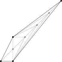
Figure 2. A resolution of $X^{5,3}$

7.4. Toric crepant resolutions

Let $X_{\Delta}$ be a toric Kähler cone. If $n=3$ then Proposition 6.8 implies that $X_{\Delta}$ admits a toric crepant resolution, $\pi:X_{\tilde{\Delta}}\rightarrow X_{\Delta}$. And more generally, if $n>3$, then $X_{\Delta}$ admits a toric partial crepant resolution $\pi:X_{\tilde{\Delta}}\rightarrow X_{\Delta}$ which has at most orbifold singularities. The author does not have a general result on the existence of a compact strictly convex support function on $\tilde{\Delta}$. Nevertheless, it is elementary to construct examples, such as in Figure 3, which has a 4-dimensional space of asymptotically conical Ricci-flat Kähler metrics. In this example $X_{\Delta}$ has another resolution, Figure 4, which is related to Figure 3 by a flop.

It is proved in [39] that for $n=3$, as long as $X$ is not the quadric cone, there is a crepant resolution $\pi:X_{\tilde{\Delta}}\rightarrow X_{\Delta}$ such that $\tilde{\Delta}$ has a compact strictly upper convex support function. And therefore, Corollary 1.3 applies. This can be used to easily construct infinitely many 3-dimensional examples.

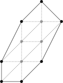
Figure 3. Example

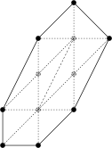
Figure 4. a flop of 3

References

- [1] Miguel Abreu. Kähler geometry of toric manifolds in symplectic coordinates. In Symplectic and contact topology: interactions and perspectives (Toronto, ON/Montreal, QC, 2001), volume 35 of Fields Inst. Commun., pages 1–24. Amer. Math. Soc., Providence, RI, 2003.
- [2] Shigetoshi Bando, Atsushi Kasue, and Hiraku Nakajima. On a construction of coordinates at infinity on manifolds with fast curvature decay and maximal volume growth. Invent. Math., 97(2):313–349, 1989.
- [3] Charles Boyer and Krzysztof Galicki. 3-Sasakian manifolds. In Surveys in differential geometry: essays on Einstein manifolds, Surv. Differ. Geom., VI, pages 123–184. Int. Press, Boston, MA, 1999.
- [4] Charles Boyer, Krzysztof Galicki, and Santiago Simanca. The Sasaki cone and extremal Sasakian metrics. In Riemannian Topology and Geometric Structures on Manifolds: in honor of Charles P. Boyer’s 65th birthday, volume 271 of Progress in Math., pages 263–290. Birkhaüser Verlag, Boston, MA, 2008.
- [5] Charles P. Boyer and Krzysztof Galicki. Sasakian geometry, hypersurface singularities, and Einstein metrics. Rend. Circ. Mat. Palermo (2) Suppl., (75):57–87, 2005.
- [6] Charles P. Boyer and Krzysztof Galicki. Sasakian geometry. Oxford Mathematical Monographs. Oxford University Press, Oxford, 2008.
- [7] Charles P. Boyer, Krzysztof Galicki, and János Kollár. Einstein metrics on spheres. Ann. of Math. (2), 162(1):557–580, 2005.
- [8] D. Burns. On rational singularities in dimensions . Math. Ann., 211:237–244, 1974.
- [9] Dan Burns, Victor Guillemin, and Eugene Lerman. Kähler metrics on singular toric varieties. Pacific J. Math., 238(1):27–40, 2008.
- [10] E. Calabi. Métriques kählériennes et fibrés holomorphes. Ann. Sci. École Norm. Sup. (4), 12(2):269–294, 1979.
- [11] Philip Candelas and Xenia C. de la Ossa. Comments on conifolds. Nuclear Phys. B, 342(1):246–268, 1990.
- [12] Yat-Ming Chan. Desingularizations of Calabi-Yau 3-folds with a conical singularity. Q. J. Math., 57(2):151–181, 2006.
- [13] Shiu Yuen Cheng and Shing Tung Yau. On the existence of a complete Kähler metric on noncompact complex manifolds and the regularity of Fefferman’s equation. Comm. Pure Appl. Math., 33(4):507–544, 1980.
- [14] Koji Cho, Akito Futaki, and Hajime Ono. Uniqueness and examples of compact toric Sasaki-Einstein metrics. Comm. Math. Phys., 277(2):439–458, 2008.
- [15] A. Futaki, H. Ono, and G. Wang. Transverse Kähler geometry of Sasaki manifolds and toric Sasaki-Einstein manifolds. arXiv:math.DG/0607586 v.5, to appear in J. Diff. Geo., 2007.
- [16] Jerome P. Gauntlett, Dario Martelli, James Sparks, and Daniel Waldram. A new infinite class of Sasaki-Einstein manifolds. Adv. Theor. Math. Phys., 8(6):987–1000, 2004.
- [17] Jerome P. Gauntlett, Dario Martelli, James Sparks, and Daniel Waldram. Sasaki-Einstein metrics on . Adv. Theor. Math. Phys., 8(4):711–734, 2004.
- [18] David Gilbarg and Neil S. Trudinger. Elliptic partial differential equations of second order, volume 224 of Grundlehren der Mathematischen Wissenschaften [Fundamental Principles of Mathematical Sciences]. Springer-Verlag, Berlin, second edition, 1983.
- [19] Hans Grauert. Über Modifikationen und exzeptionelle analytische Mengen. Math. Ann., 146:331–368, 1962.
- [20] Victor Guillemin. Kaehler structures on toric varieties. J. Differential Geom., 40(2):285–309, 1994.
- [21] Victor Guillemin. Moment maps and combinatorial invariants of Hamiltonian -spaces, volume 122 of Progress in Mathematics. Birkhäuser Boston Inc., Boston, MA, 1994.
- [22] Dominic Joyce. Asymptotically locally Euclidean metrics with holonomy . Ann. Global Anal. Geom., 19(1):55–73, 2001.
- [23] Dominic D. Joyce. Compact manifolds with special holonomy. Oxford Mathematical Monographs. Oxford University Press, Oxford, 2000.
- [24] János Kollár and Shigefumi Mori. Birational geometry of algebraic varieties, volume 134 of Cambridge Tracts in Mathematics. Cambridge University Press, Cambridge, 1998. With the collaboration of C. H. Clemens and A. Corti, Translated from the 1998 Japanese original.
- [25] P. B. Kronheimer. The construction of ALE spaces as hyper-Kähler quotients. J. Differential Geom., 29(3):665–683, 1989.
- [26] Henry B. Laufer. On rational singularities. Amer. J. Math., 94:597–608, 1972.
- [27] Eugene Lerman. Contact toric manifolds. J. Symplectic Geom., 1(4):785–828, 2003.
- [28] Dario Martelli and James Sparks. Toric Sasaki-Einstein metrics on . Phys. Lett. B, 621(1-2):208–212, 2005.
- [29] Dario Martelli and James Sparks. Resolutions of non-regular Ricci-flat Kähler cones. arXiv:math.DG/0707.1674 v.2, 2007.
- [30] Dario Martelli and James Sparks. Baryonic branches and resolutions of Ricci-flat Kähler cones. J. High Energy Phys., (4):067, 44, 2008.
- [31] Dario Martelli and James Sparks. Symmetry-breaking vacua and baryon condensates in AdS/CFT correspondence. Phys. Rev. D, 79(6):065009, 51, 2009.
- [32] Dario Martelli, James Sparks, and Shing-Tung Yau. The geometric dual of -maximisation for toric Sasaki-Einstein manifolds. Comm. Math. Phys., 268(1):39–65, 2006.
- [33] Yozô Matsushima. Sur la structure du groupe d’homéomorphismes analytiques d’une certaine variété kählérienne. Nagoya Math. J., 11:145–150, 1957.
- [34] Tadao Oda. Convex bodies and algebraic geometry, volume 15 of Ergebnisse der Mathematik und ihrer Grenzgebiete (3) [Results in Mathematics and Related Areas (3)]. Springer-Verlag, Berlin, 1988. An introduction to the theory of toric varieties, Translated from the Japanese.
- [35] Liviu Ornea and Misha Verbitsky. Embeddings of compact Sasakian manifolds. Math. Res. Lett., 14(4):703–710, 2007.
- [36] Shi-Shyr Roan. Minimal resolutions of Gorenstein orbifolds in dimension three. Topology, 35(2):489–508, 1996.
- [37] Gang Tian and Shing-Tung Yau. Complete Kähler manifolds with zero Ricci curvature. I. J. Amer. Math. Soc., 3(3):579–609, 1990.
- [38] Gang Tian and Shing-Tung Yau. Complete Kähler manifolds with zero Ricci curvature. II. Invent. Math., 106(1):27–60, 1991.
- [39] Craig van Coevering. Examples of asymptotically conical Ricci-flat Kähler manifolds. arXiv:math.DG/0812.4745 v.2, to appear in Math. Z., 2008.
- [40] Craig van Coevering. A construction of complete Ricci-flat Kähler manifolds. arXiv:math.DG/0803.0112 v.3, 2009.
- [41] Xu-Jia Wang and Xiaohua Zhu. Kähler-Ricci solitons on toric manifolds with positive first Chern class. Adv. Math., 188(1):87–103, 2004.