Long Term Evolution of Magnetized Bubbles in Galaxy Clusters

Abstract

We have performed nonlinear ideal magnetohydrodynamic simulations of the long term evolution of a magnetized low-density “bubble” plasma formed by a radio galaxy in a stratified cluster medium. It is found that about 3.5% of the initial magnetic energy remains in the bubble after $\sim 8\times 10^{9}$ years, and the initial magnetic bubble expansion is adiabatic. The bubble can survive for at least $8\times 10^{9}$ years due to the stabilizing effect of the bubble magnetic field on Rayleigh-Taylor and Kelvin-Holmholtz instabilities, possibly accounting for “ghost cavities” as observed in Perseus-A. A filament structure spanning about 500 kpc is formed along the path of bubble motion. The mean value of the magnetic field inside this structure is $\sim 0.88$ $\mu$G at $\sim 8\times 10^{9}$ years. Finally, the initial bubble momentum and rotation have limited influence on the long term evolution of the bubble.

1 Introduction

An unsolved problem in active galactic nuclei (AGN) feedback on clusters is how to account for the the morphology and stability of buoyant bubbles and their interactions with the ambient intracluster medium (ICM) (McNamara & Nulsen, 2007). Fabian et al. (2006) showed that in the Perseus cluster, such bubbles can stay intact far from cluster centers where they were inflated by AGN jets. However, studies of kinetic-energy dominated jets in the purely hydrodynamic limit did not explain the observed long term persistence of the buoyant bubbles, which are prone to Rayleigh-Taylor (RTI) and Kelvin-Holmhotz (KHI) instabilities and fragment entirely within $100\;\,{\rm Myr}$, contrary to observations [but see Reynolds et al. (2005); Pizzolato & Soker (2006); Gardini (2007)].

Appreciable magnetic energy has been observed in both cluster and radio lobe plasmas (Owen et al., 2000; Kronberg et al., 2001; Croston et al., 2005). The magnetic fields could play a vital role in the dynamics of the rising bubble, as shown by a series of 2D magnetohydrodynamic (MHD) studies for bubbles of several $10^{8}$ years (Brüggen & Kaiser, 2001; Robinson et al., 2004; Jones & De Young, 2005). Stone & Gardiner (2008) showed that uniform strong magnetic fields do not suppress RTI completely, but sheared fields at the bubble interface quench the instability. This implies that not only the field strength but also the configuration matters for bubble stability. Ruszkowski et al. (2007) did a comprehensive study of the influence of different magnetic field configurations upon the stability of a rising bubble. They found that the internal bubble helical magnetic field moderately stabilizes the bubble, however the bubble has an initial plasma parameter $\beta\equiv\left<2nT/B^{2}\right>\gg 1$, still in thermal energy-dominated regime. Recently, Li et al. (2006) proposed a different bubble magnetic field configuration for jet/lobes. Here we adopt the field configuration of Li et al. (2006) and focus on the late stage of the evolution of magnetically dominated bubbles in 3D. We show that this spheromak-like magnetic field configuration strongly stabilizes the instabilities and prevents the bubble from breaking up, possibly forming the intact but detached “ghost cavity” observed in systems such as Perseus-A. This Letter is organized as follows. In Sec. 2, we describe the problem setup. The simulation results and discussions are given in Sec. 3.

2 Problem Set Up

The background ICM is assumed to be hydrostatic and isothermal. The density and pressure profile is given as $\rho=p=[1+(R/R_{c})^{2}]^{-\kappa}$, where the parameters $\kappa$ and $R_{c}$ are taken to be $1.0$ and $4.0$ respectively. The fixed yet distributed gravitational field $-\nabla\psi(R)$ dominated by the dark matter is assumed (Nakamura et al., 2006). We simulate only the phase after the AGN has inflated a low-density bubble which is in pressure equilibrium with the ICM initially. The static magnetized bubble initially lies at $(x_{b},y_{b},z_{b})=(0,0,5)$ with density $\rho_{b}=0.1$, spherical radius $r_{d}=2$ for the density profile and $r_{b}=1$ for the magnetic configuration. The specific heat $\gamma$ inside and outside the bubble is taken to be $5/3$. Physical quantities are normalized by the characteristic system length scale $R_{0}=25\;\,{\rm kpc}$, density $\rho_{0}=1.67\times 10^{-26}\;\,{\rm g\;cm^{-3}}$, and velocity $V_{0}=6.2\times 10^{7}\;\,{\rm cm\;s^{-1}}$. The initial sound speed, $C_{s}|_{t=0}=\gamma^{1/2}\sim 1.29$, is constant throughout the computational domain. Other quantities are normalized as: time $t=1$ gives $R_{0}/V_{0}=38.6\;\,{\rm Myr}$, magnetic field $B=1$ gives $(2\rho_{0}V_{0}^{2})^{1/2}=1.13\times 10^{-5}\;\,{\rm G}$ and energy $E=1$ gives $\rho_{0}V_{0}^{2}R_{0}^{3}=2.71\times 10^{58}\;\,{\rm ergs}$. The magnetic field setup of the bubble follows Li et al. (2006) with the ratio of toroidal to poloidal bubble field $\alpha$ taken to be $\sqrt{10}$, which corresponds to a minimum initial Lorentz force. The latter is reasonable since we want to mimic the situation that the magnetic bubble has substantially relaxed and detached from the jet tip. The initial total magnetic energy is around $2.0\times 10^{59}\;\,{\rm ergs}$. The computational domain is taken to be $|x|\leq 16$, $|y|\leq 16$, and $0\leq z\leq 32$ corresponding to a $(800\;\,{\rm kpc})^{3}$ box in the actual length scales. The numerical resolution used here is $400^{3}$, where the grid points are assigned uniformly in every direction. A cell $\delta x$ corresponds to $2.0\;\,{\rm kpc}$. We use “outflow” boundary conditions at every boundary except the boundary at $z=0$, where we use “reflecting” boundary conditions, which guarantee that the energy flux through this boundary is zero.

3 Results & Discussion

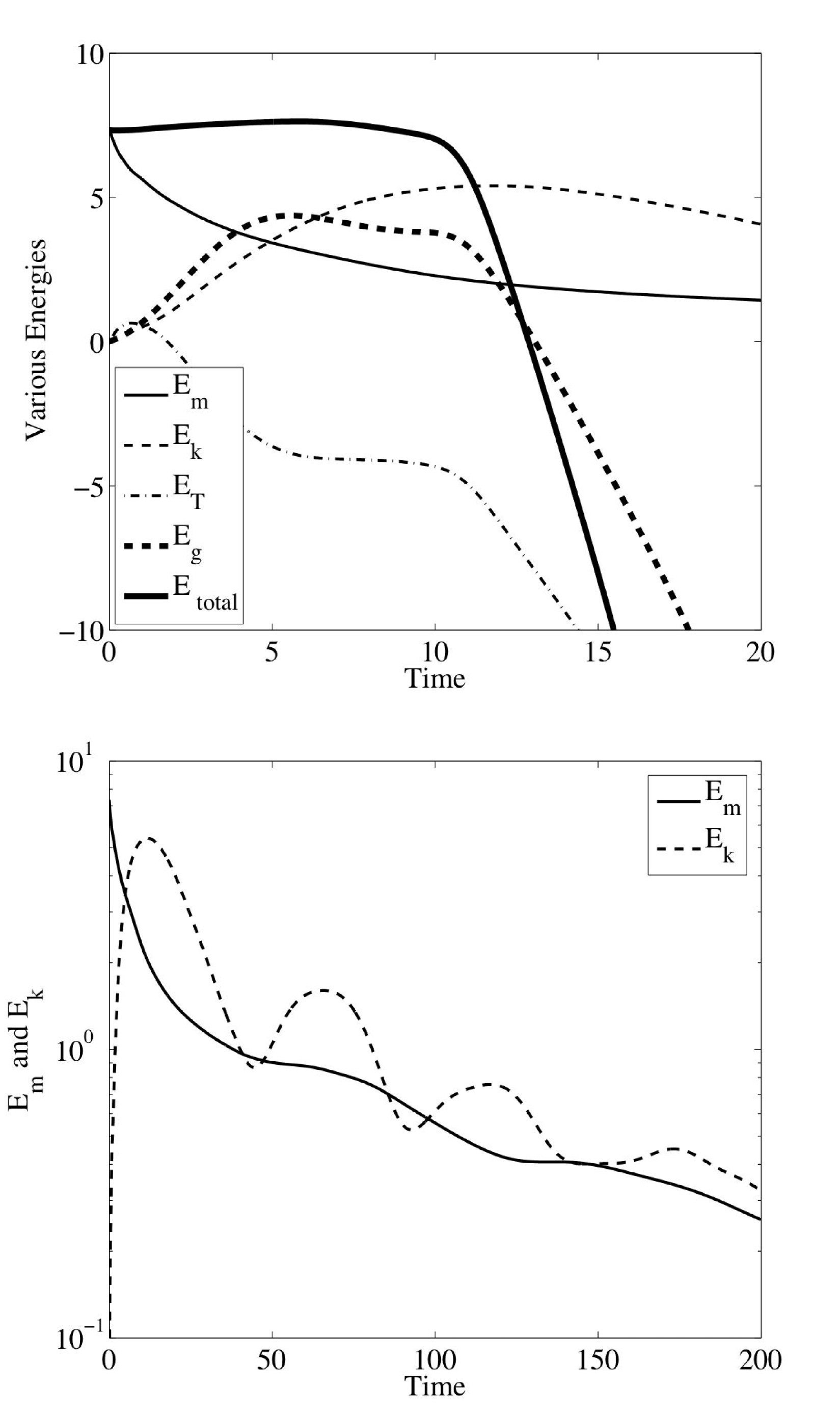
Figure 1:  Time evolution of various energies. Top: short term various energies evolution $t\leq 20$, thin solid: magnetic Energy $E_{m}$, thin dash: kinetic energy $E_{k}$, thin dash dot: internal energy $E_{T}$, thick dash: gravitational energy $E_{g}$ and thick solid: total energy $E_{\rm tol}$. Bottom: long term time evolution of magnetic energy (in logarithmic scale) $E_{m}$ (solid) and kinetic energy $E_{k}$ (dash). $t=1$ represents $38.6\;\,{\rm Myr}$.

Energy and density evolution reveal the different stages of the bubble. Figure 1(top) presents the time evolution of various energies at the early stage, in which the gravitational energy $E_{g}=\int\rho\psi dV$ and the internal energy $E_{T}=\int p/(\gamma-1)dV$, where $dV$ is the infinitesimal volume and the integral is over the entire computation domain, have been reduced by their initial values $E_{g,0}$ and $E_{T,0}$, respectively. The total energy is defined as $E_{\rm total}=E_{m}+E_{k}+E_{T}+E_{g}$, where the kinetic energy is defined as $E_{k}=\int 1/2\rho v^{2}dV$ and the magnetic energy is defined as $E_{m}=\int B^{2}/2dV$. At the early stage ($t\lesssim 5$), the kinetic energy increases since the bubble accelerates upward due to buoyancy, and the magnetic energy decreases due to work done in expansion from the weak initial Lorentz force and conversion to shock and wave energy (Nakamura et al., 2006). The gravitational energy increases because there is a net outward mass flow in the axial direction. The passage of the shock wave heats and compresses the ICM and alters its pressure gradient. The total energy $E_{\rm total}$ is almost constant before $t\sim 10$, at which time the shock and wavefront reach the boundary. Conservation of the total energy for $t\lesssim 10$ is not strictly satisfied due to numerical diffusion. The initial bubble expansion ($t\leq 20$) is approximately adiabatic, which gives $E=Vp\propto V^{1-\gamma}$, where $V$ is the bubble volume. Therefore $E_{2}/E_{1}=(V_{1}/V_{2})^{2/3}$, where the subscript $1$ and $2$ indicate the initial and final state, respectively. At $t=20$, the radius of the bubble has increased from $2$ to $\sim 5$, which gives $E_{2}/E_{1}\sim 16\%$, roughly matching the amount of magnetic energy in the bubble [$20\%$ from Fig. 1(top)]. For later times [Fig. 1(bottom)], fitting with $E_{m}(t)/E_{m,0}=\exp(-t/\tau_{\rm dis})$, we have: (1) a fast dissipation stage ($t\lesssim 10$) when magnetic energy dissipation time $\tau_{\rm dis}\sim 11$; (2) a slow dissipation stage ($t\gtrsim 10$) when $\tau_{\rm dis}\sim 114$. Both times are much smaller than the numerical dissipation time $\tau_{\rm res}$ at the corresponding stages (see discussions at the end of this section). The kinetic energy is oscillating while it is decaying slowly, which can be understood as follows. Gravity pulls the bubble down to the denser ICM, compressing the bubble and causing an increase in magnetic energy (since the magnetic flux is nearly conserved). This results in the magnetic energy oscillating in phase with the kinetic energy with period $\sim 90$ ($3.5\times 10^{9}\;\,{\rm yr}$). At $t=200$ after several periods of decaying oscillations, about 3.5% of the initial magnetic energy remains.

The magnetic field suppresses instabilities and therefore the bubble remains intact longer. Figure 2 presents the typical density distribution (logarithmic scale) in 2D $x$–$z$ slices at $y=0$ at different times ($t=0,7.5,20,50,100,125$). The white solid contour lines indicate contours of constant magnetic field strength $|B|$. Consistent with Fig. 1(bottom), after $t\gtrsim 50$, the bubble undergoes a slowly decaying oscillation between $z\sim 19$ and $z\sim 24$. We have also performed simulations of an unmagnetized bubble and found that it disintegrates after $t=20$, whereas the magnetic bubble still clearly differentiates itself from the ambient medium at $t=200$ (Fig. 2). The formation of an “umbrella” or a thin protective magnetic layer on the bubble working surface suppresses instabilities (Ruszkowski et al., 2007). The stronger magnetic field is also found to move the bubble faster and push the bubble farther away from its initial position. The position of the bubble top as a function of time is shown in Fig. 3. This position is calculated by plotting the axial profile of the density along the line of $(x,y)=(0,0)$ and finding the location of the first density jump from the top of the domain. Comparing the unmagnetized run (dash line) with the magnetized run (both without initial momentum/rotation), we can see that the rising speed increases from $~{}0.36$ to $0.6$. Note that the rough estimate of the terminal speed $v_{t}$ based on the initial gravitational acceleration $g$ and size $r_{d}$, both position-dependent, is $v_{t}\approx 4/3\sqrt{2gr_{d}}\sim 2$, assuming force balance between buoyancy and viscous drag force at the final stage (McNamara & Nulsen, 2007).

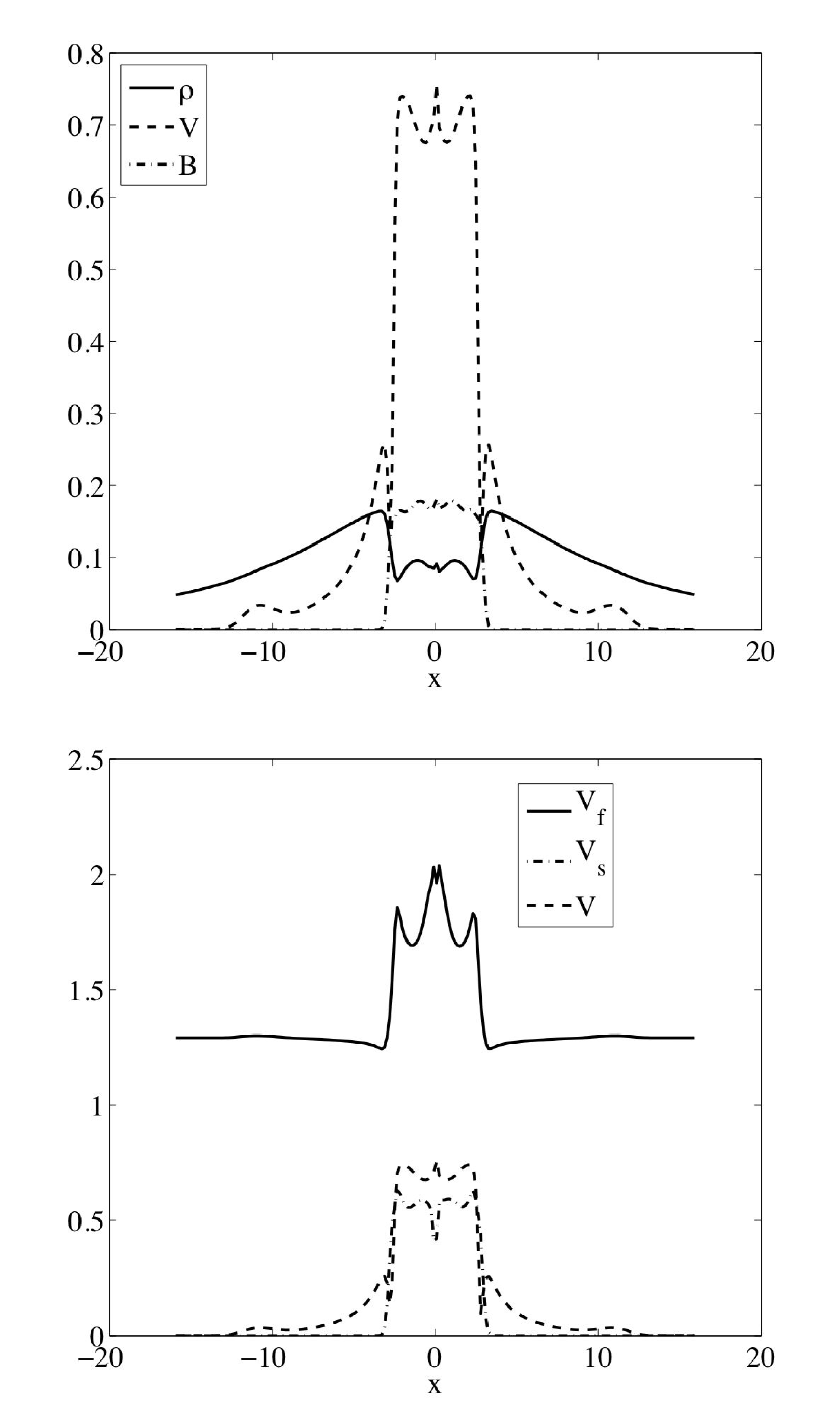
Figure 4:  Transverse profiles in the $x$-direction of several quantities at $t=7.5$ on $z=8.0$. The bulk speed $V$, the density $\rho$, and the magnetic field strength $B$ are shown for inspecting the KHI surface modes (top). The bulk speed $V$, the superfast magnetosonic speed $V_{f}$, and the slow magnetosonic speed $V_{s}$ are shown for inspecting the KHI body modes (bottom).

We investigate the effect of the magnetic field on bubble stability in more detail. Following Nakamura et al. (2007), we first study KHI of the bubble. At both sides of the bubble, the magnetic field is almost uniform, not twisted like at the top of the bubble. From linear analysis, the instability criterion for nonaxisymmetric KHI surface modes is (Hardee & Rosen, 2002) : $\Delta V>V_{As}=[(\rho_{b}+\rho_{e})/(4\pi\rho_{b}\rho_{e})(B_{b}^{2}+B_{e}^{2})]^{1/2}$, where $\Delta V\equiv|V_{b}-V_{e}|$ is the velocity shear and $V_{As}$ is the surface Alfvén speed. The subscripts $b$ and $e$ indicate the bubble and external medium, respectively. The nonaxisymmetric body modes would be important if (Hardee & Rosen, 1999): (1) $V_{b}>V_{f}$, in which $V_{f}$ is the fast magnetosonic speed; or (2) $C_{s}V_{A}/(C_{s}^{2}+V_{A}^{2})^{1/2}<V_{b}<V_{s}$, in which $V_{A}$ is the Alfvén speed and $V_{s}$ is the slow magnetosonic speed. The definitions of $V_{f,s}$ are: $V_{f,s}=\big{\{}1/2\{C_{s}^{2}+V_{A}^{2}\pm[(C_{s}^{2}+V_{A}^{2})^{2}-4C_{s}^{2}V_{A}^{2}\cos^{2}\theta]^{1/2}\}\big{\}}^{1/2}$. Since we focus on the $x$-direction only, $V_{A}^{2}\cos^{2}\theta$ are taken to be $B_{x}^{2}/\rho$. Figure 4 (top) displays the transverse distribution of the bulk flow speed $V=(v_{x}^{2}+v_{y}^{2}+v_{z}^{2})^{1/2}$, the density $\rho$, and the magnetic field strength $B$ at $t=7.5$ at $z=8.0$. A distinct velocity shear is identified at $x\sim 3.5$. Across this shear, $\Delta V\sim 0.75$ and $V_{As}\sim 0.85$. The inequality $\Delta V<V_{As}$ holds. This means that the KHI surface modes are completely suppressed. Figure 4 (bottom) displays the transverse distribution of $V$, $V_{f}$, and $V_{s}$ at $t=7.5$ at $z=8.0$ . We see that the bulk flow $V$ lies between $V_{f}$ and $V_{s}$. The inequality $V_{s}<V<V_{f}$ is satisfied in the body of the buoyant bubble. This rules out the KHI body modes as well.

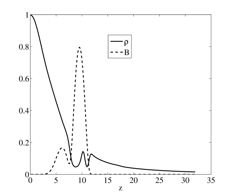
Figure 5:  Axial profiles in the $z$-direction of several quantities at $t=7.5$ with $(x,y)=(0,0)$. The density $\rho$ and the magnetic field strength $B$ are shown for inspecting the RTI modes.

RTI could also be suppressed by the magnetic field. For the idealized case of two conducting fluids separated by a contact discontinuity with a uniform magnetic field parallel to the interface undergoing constant acceleration $g$, Chandrasekhar (1961) demonstrated that RTI on a scale $L$ parallel to the field requires $B<B_{c}\equiv[Lg(\rho_{h}-\rho_{l})]^{1/2}$, in which $\rho_{h}$ and $\rho_{l}$ are the densities in the heavy and light fluids respectively. Modes perpendicular to the field are unaffected. At the top of the bubble ($z\sim 11.6$) (Fig. 5), $\rho_{h}$ and $\rho_{l}$ are found to be $0.15$ and $0.06$, respectively, and the gravitational acceleration $g$ is calculated to be $0.95$. If $L$ is chosen to be the computation domain size, the maximum possible mode wavelength in the simulations, then the critical magnetic field strength is $B_{c}\sim 1.6$, which is larger than the magnetic field ($\sim 0.8$) at that location. This means that only part of the parallel modes are suppressed regardless of the perpendicular modes. This is not consistent with the simulation results. However, as pointed out in Stone & Gardiner (2008), the twisting nature of the bubble field at the top of the bubble introduces a current sheet at the surface, and the changes in the direction of the field at the interface must be on very small scales to inhibit the interchange modes. A more detailed study of this effect is beyond the scope of this paper and will be the subject of future study.

Our simulation also provides one possible explanation of the morphology and origin of the large scale magnetic field and the generation of “ghost cavities” observed in many clusters. Like Robinson et al. (2004), a magnetized high-density tail remains as the bubble rises (Fig. 2). The tails have an elongated morphology (Fig. 2), resembling H$\alpha$ filaments, which is found to indicate the history of the rising bubble. Interestingly, the magnetic field also helps stabilize this “filament” as it is still visible at $t=200$. Nipoti & Binney (2004) has argued that thermal conduction has to be strongly suppressed in the ICM; otherwise, such cold filaments would be rapidly evaporated. As in Ruszkowski et al. (2007), our results provide a possibility that thermal conduction may be locally weaker in the bubble wake, thus preventing or slowing down filament evaporation. The magnetic field is distributed between $z\sim 2.5$ and $z\sim 25$ at $t=200$ with peak value around $0.156$ ($\sim 1.8\;\,{\rm\mu G}$) or mean value around $0.078$ ($\sim 0.88\;\,{\rm\mu G}$), close to the estimates of wider cluster fields (Carrili & Taylor, 2002; Taylor et al., 2002). This large-scale ($\gtrsim 500\;\,{\rm kpc}$) magnetic field structure also mimics the morphology of the second class (“Phoenix”) of “radio relics” elongated from the cluster center to the periphery observed in A 115 (Govoni et al., 2001). The simulation results mean that the magnetic bubble rising from $\sim 125\;\,{\rm kpc}$ with an initial magnetic energy of $2\times 10^{59}\;\,{\rm ergs}$, will spread magnetic fields between $62.5\;\,{\rm kpc}\lesssim z\lesssim 600\;\,{\rm kpc}$ and keep a magnetized bubble between $475\;\,{\rm kpc}$ and $600\;\,{\rm kpc}$ for at least $\sim 8\times 10^{9}\;\,{\rm yr}$. Therefore one could reproduce the intact but detached “ghost cavity” observed in some systems such as Perseus-A.

Real radio lobes possess complex, jet-driven flows, different from the static bubble that we use for our initial conditions. We study the effects of additional variations in the initial bubble by having: (1) an initial uniform injection speed $v_{\rm inj}$ or (2) an initial uniform rotation $\omega$. Nakamura et al. (2008) reported that the radio lobe gains a momentum of $v_{\rm inj}\sim 0.91C_{s0}=1.174$, and the rotation speed $\omega$ at the edge of the bubble reaches $\sim 1.5C_{s0}/r_{d}=0.9675$ after jet-driven inflation and interaction with the ambient ICM, although neither are not uniform inside the bubble. Here we take these two values as our initial values for $v_{\rm inj}$ and $\omega$ and idealize both to be uniform throughout the bubble. Fig. 3 presents the time evolution of the position of the bubble top with initial uniform injection velocity $v_{\rm inj}=1.174$ (long dash) and initial uniform rotation speed $\omega=0.9675$ (dash dot). It is seen that these two variables only have some influence on the evolution of the bubble during the early stage. The bubble with an initial rotation has a reduced buoyancy resulting from rotation-driven instabilities that in turn lead to a reduced pressure differential between the bubble and the ICM. The evolution, and structure of the bubble in the later times are, however, essentially the same.

The effects of numerical diffusion are estimated as follows. If we fit the net toroidal magnetic flux $\psi_{t}=\int B_{y}dS$ (only positive $B_{y}$ is selected) as $\psi_{t}(t)/\psi_{t}(t=0)\equiv\exp(-t/\tau_{\rm res})$, the “resistive” dissipation time due to numerical diffusion is $\tau_{\rm res}\sim 38$ for $t\leq 10$, $\tau_{\rm res}=138$ for $10\leq t\leq 50$, and $\tau_{\rm res}=507$ for $50\leq t\leq 100$. Therefore the numerical diffusion is not important on the time scales of interest $(t\lesssim 200)$. Increasing numerical resolution can further reduce the numerical diffusion.

The oldest bubbles known so far are a few hundred $\,{\rm Myr}$ old (McNamara & Nulsen, 2007), which are much younger than the long-sustained ($\sim$ a Hubble time) magnetized bubbles reported in this Letter. The simulations show that at later times $t\gtrsim 50$, the density and X-ray luminosity contrast between the bubble and ICM plasma at the periphery of the cluster is small, which makes the direct X-ray observation of the bubble faraway from the parent galaxy very difficult. But the radio bubble at the borders of the clusters may still be detectable through: (1) Faraday rotation measurement of the outskirts of the cluster if an outside synchrotron source exists; (2) or radio observation from re-energization of fossil radio bubble plasma by shocks or mergers. It is highly possible for the bubbles to pile up in the outer atmospheres of the clusters in deep Chandra observation, if those observations are technically viable.

It is conceivable that part of the initial magnetic energy of the bubble accelerates cosmic rays. Throughout the lifetime of a cluster, there could be multiple AGNs injecting jets/lobes into the ICM. Both the cosmic rays and the remaining magnetic fields (distributed over large scales) could provide the energy sources for phenomena such as radio relics and radio haloes that have been observed for a number of clusters (Ferrari et al., 2008).

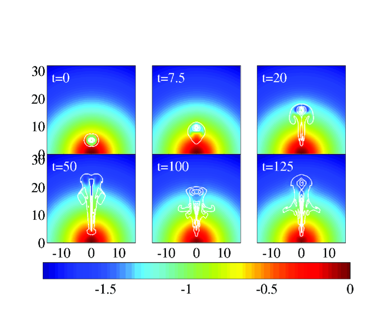
Figure 2:  (color) Density (in logarithmic scale) in the $x$-$z$ plane as a function of time ($\alpha=\sqrt{10}$). The white solid contour lines indicate the magnetic field strength $|B|$. $t=0$, $|B|\in[0,1.976]$; $t=7.5$, $|B|\in[0,0.830]$; $t=20$, $|B|\in[0,0.400]$; $t=50$, $|B|\in[0,0.328]$; $t=100$, $|B|\in[0,0.159]$; $t=125$, $|B|\in[0,0.156]$. $|B|=1$ represents $11.3\;\,{\rm\mu G}$. The number of the contour levels are all $5$.

Figure 3:  Position of the bubble top v.s. time for four different runs. The solid, long dash and dash dot lines represent magnetized bubble runs without initial momentum rotation, with $v_{\rm inj}=1.174$ and with $\omega=0.9675$ respectively. The short dash line denotes the purely hydrodynamic run.

References

- Brüggen & Kaiser (2001) Brüggen, M. & Kaiser, C. R. 2001, MNRAS, 325, 676
- Carrili & Taylor (2002) Carrili, C. L. & Taylor, G. B. 2002, ARA&A, 40, 319
- Chandrasekhar (1961) Chandrasekhar, S. 1961, Hydrodynamic and Hydromagnetic Stability (Oxford University Press)
- Croston et al. (2005) Croston et al. 2005, Astrophys. J., 626, 733
- Fabian et al. (2006) Fabian et al. 2006, MNRAS, 367, 433
- Ferrari et al. (2008) Ferrari et al. 2008, Space Sci. Rev., 134, 93
- Gardini (2007) Gardini, A. 2007, A&A, 464, 143
- Govoni et al. (2001) Govoni et al. 2001, A&A, 376, 803
- Hardee & Rosen (1999) Hardee, P. E. & Rosen, A. 1999, ApJ, 524, 650
- Hardee & Rosen (2002) —. 2002, ApJ, 576, 204
- Jones & De Young (2005) Jones, T. W. & De Young, D. S. 2005, ApJ, 624, 586
- Kronberg et al. (2001) Kronberg, P. P., Dufton, Q. W., Li, H., & Colgate, S. A. 2001, Astrophys, J., 560, 178
- Li et al. (2006) Li, H., Lapenta, G., Finn, J. M., Li, S., & Colgate, S. A. 2006, Astrophys. J., 643, 92
- McNamara & Nulsen (2007) McNamara, B. R. & Nulsen, P. E. J. 2007, ARA&A, 45, 117
- Nakamura et al. (2006) Nakamura, M., Li, H., & Li, S. 2006, Astrophys. J., 652, 1059
- Nakamura et al. (2007) —. 2007, Astrophys. J., 656, 721
- Nakamura et al. (2008) Nakamura, M., Tregillis, I. L., Li, H., & Li, S. 2008, ApJ, in press
- Nipoti & Binney (2004) Nipoti, C. & Binney, J. 2004, MNRAS, 349, 1509
- Owen et al. (2000) Owen, F. N., Eilek, J. A., & Kassim, N. E. 2000, Astrophys. J., 543, 611
- Pizzolato & Soker (2006) Pizzolato, F. & Soker, N. 2006, Mon. Not. R. Astron. Soc., 371, 1835
- Reynolds et al. (2005) Reynolds, C. S., McKernan, B., Fabian, A. C., & Stone, J. M. 2005, MNRAS, 357, 242
- Robinson et al. (2004) Robinson et al. 2004, ApJ, 601, 621
- Ruszkowski et al. (2007) Ruszkowski et al. 2007, MNRAS, 378, 662
- Stone & Gardiner (2008) Stone, J. M. & Gardiner, T. 2008, ApJ, in press
- Taylor et al. (2002) Taylor, G. B., Fabian, A. C., & Allen, S. W. 2002, MNRAS, 334, 769