Duality of real and quaternionic random matrices

Abstract.

We show that quaternionic Gaussian random variables satisfy a generalization of the Wick formula for computing the expected value of products in terms of a family of graphical enumeration problems. When applied to the quaternionic Wigner and Wishart families of random matrices the result gives the duality between moments of these families and the corresponding real Wigner and Wishart families.

1. Introduction

The duality between symplectic and orthogonal groups has a long standing history, and has been noted in physics literature in various settings, see e.g. [15, 20, 25, 27]. Informally, the duality asserts that averages such as moments or partition functions for the symplectic case of “dimension” $N$, can be derived from the respective formulas for the orthogonal case of dimension $N$ by inserting $-N$ into these expressions and by simple scaling. The detailed study of the moments of one-matrix Wishart ensembles, with duality explicitly noted, appears in [10], see [10, Corollary 4.2]. The duality for one matrix Gaussian Symplectic Ensemble was noted by Mulase and Waldron [21] who introduced Möbius graphs to write the expansion for traces of powers of GOE/GUE/GSE expansions in a unified way. The duality appears also in [17, Theorem 6] as a by-product of differential equations for the generating functions of moments. Ref. [6, 7, 8] analyze the related “genus series” over locally orientable surfaces.

The purpose of this paper is to prove that the duality between moments of the Gaussian Symplectic Ensemble and the Gaussian Orthogonal Ensemble, and between real Wishart and quaternionic Wishart ensembles extends to several independent matrices. Our technique consists of elementary combinatorics; our proofs differ from [21] in the one matrix case, and provide a more geometric interpretation for the duality; in the one-matrix Wishart case, our proof completes the combinatorial approach initiated in [10, Section 6]. The technique limits the scope of our results to moments, but the relations between moments suggest similar relations between other analytic objects, such as partition functions, see [21], [16]. The asymptotic expansion of the partition function and analytic description of the coefficients of this expansion for $\beta=2$ case appear in [4, 9, 19].

The paper is organized as follows. In Section 2 we review basic properties of quaternionic Gaussian random variables. In Section 3 we introduce Möbius graphs; Theorems 3.1 and 3.2 give formulae for the expected values of products of quaternionic Gaussian random variables in terms of the Euler characteristics of sub-families of Möbius graphs or of bipartite Möbius graphs. In Section 4 we apply the formulae to the quaternionic Wigner and Wishart families.

In this paper, we do not address the question of whether the duality can be extended to more general functions, or to more general $\beta$-Hermite and $\beta$-Laguerre ensembles introduced in [3].

2. Moments of quaternion-valued Gaussian random variables

2.1. Quaternion Gaussian law

Recall that a quaternion $q\in\mathbb{H}$ can be represented as $q=x_{0}+ix_{1}+jx_{2}+kx_{3}$ with $i^{2}=j^{2}=k^{2}=ijk=-1$ and with real coefficients $x_{0},\dots,x_{3}$. The conjugate quaternion is $\overline{q}=x_{0}-ix_{1}-jx_{2}-kx_{3}$, so $|q|^{2}:=q\overline{q}\geq 0$. Quaternions with $x_{1}=x_{2}=x_{3}=0$ are usually identified with real numbers; the real part of a quaternion is $\Re(q)=(q+\bar{q})/2$.

It is well known that quaternions can be identified with the set of certain $2\times 2$ complex matrices:

(2.1) $$\mathbb{H}\ni x_{0}+ix_{1}+jx_{2}+kx_{3}\sim\left[\begin{matrix}x_{0}+ix_{1}&x_{2}+ix_{3}\\ -x_{2}+ix_{3}&x_{0}-ix_{1}\end{matrix}\right]\in\mathcal{M}_{2\times 2}(\mathbb{C}),$$

where on the right hand side $i$ is the usual imaginary unit of $\mathbb{C}$. Note that since $\Re(q)$ is twice the trace of the matrix representation in (2.1), this implies the cyclic property

(2.2) $$\Re(q_{1}q_{2}\dots q_{n})=\Re(q_{2}q_{3}\dots q_{n}q_{1}).$$

The (standard) quaternion Gaussian random variable is an $\mathbb{H}$-valued random variable which can be represented as

(2.3) $$Z=\xi_{0}+i\xi_{1}+j\xi_{2}+k\xi_{3}$$

with independent real normal $N(0,1)$ random variables $\xi_{0},\xi_{1},\xi_{2},\xi_{3}$. Due to symmetry of the centered normal laws on $\mathbb{R}$, the law of $(Z,\overline{Z})$ is the same as the law of $(\overline{Z},Z)$. A calculation shows that if $Z$ is quaternion Gaussian then for fixed $q_{1},q_{2}\in\mathbb{H}$,

$$\mathbb{E}(Zq_{1}Zq_{2})=\mathbb{E}(Z^{2})\bar{q}_{1}q_{2},\;\mathbb{E}(Zq_{1}\overline{Z}q_{2})=\mathbb{E}(Z\bar{Z})\Re(q_{1})q_{2}\,.$$

For future reference, we insert explicitly the moments:

(2.4) $$\mathbb{E}(Zq_{1}Zq_{2}) = -2\bar{q}_{1}q_{2},$$

(2.5) $$\mathbb{E}(Zq_{1}\overline{Z}q_{2}) = 2(q_{1}+\bar{q}_{1})q_{2}.$$

By linearity, these formulas imply

(2.6) $$\mathbb{E}(\Re(Zq_{1})\Re(\overline{Z}q_{2})) = \Re(q_{1}q_{2}),$$

(2.7) $$\mathbb{E}(\Re(Zq_{1})\Re(Zq_{2})) = \Re(\bar{q}_{1}q_{2}).$$

2.2. Moments

The following is known as Wick’s theorem [26].

Theorem A (Isserlis [12]).

If $(X_{1},\dots,X_{2n})$ is a $\mathbb{R}^{2n}$-valued Gaussian random vector with mean zero, then

(2.8) $$E(X_{1}X_{2}\dots X_{2n})=\sum_{V}\prod_{\{j,k\}\in V}E(X_{j}X_{k}),$$

where the sum is taken over all pair partitions $V$ of $\{1,2,\dots,2n\}$, i.e., partitions into two-element sets, so each $V$ has the form

$$V=\left\{\{j_{1},k_{1}\},\{j_{2},k_{2}\},\dots,\{j_{n},k_{n}\}\right\}.$$

Theorem A is a consequence of the moments-cumulants relation [18]; the connection is best visible in the partition formulation of [22]. For another proof, see [14, page 12].

Our first goal is to extend this formula to certain quaternion Gaussian random variables. The general multivariate quaternion Gaussian law is discussed in [24]. Here we will only consider a special setting of sequences that are drawn with repetition from a sequence of independent standard Gaussian quaternion random variables. In section 4 we apply this result to a multi-matrix version of the duality between GOE and GSE ensembles of random matrices.

In view of the Wick formula (2.8) for real-valued jointly Gaussian random variables, formulas (2.4) and (2.5) allow us to compute moments of certain products of quaternion Gaussian random variables. Suppose the $n$-tuple $(X_{1},X_{2},\dots,X_{n})$ consists of random variables taken, possibly with repetition, from the set

$$\{Z_{1},\bar{Z}_{1},Z_{2},\bar{Z_{2}},\dots\},$$

where $Z_{1},Z_{2},\dots$ are independent quaternion Gaussian random variables. Consider an auxiliary family of independent pairs $\{(Y_{j}^{(r)},Y_{k}^{(r)}):r=1,2,\dots\}$ which have the same laws as $(X_{j},X_{k})$, $1\leq j,k\leq n$ and are independent for different $r$. Then the Wick formula for real-valued Gaussian variables implies $\mathbb{E}(X_{1}X_{2}\dots X_{n})=0$ for odd $n$, and

(2.9) $$\mathbb{E}(X_{1}X_{2}\dots X_{n})=\sum_{f}\mathbb{E}(Y_{1}^{(f(1))}Y_{2}^{(f(2))}\dots Y_{n}^{(f(n))}),$$

where the sum is over the pair partitions $V$ that appear under the sum in Theorem A, each represented by the level sets of a two-to-one valued function $f:\{1,\dots,n\}\to\{1,\dots,m\}$ for $n=2m$. (Thus the sum is over classes of equivalence of $f$, each of $m!$ representatives contributing the same value.)

For example, if $Z$ is quaternion Gaussian then applying (2.9) with $f_{1}$ that is constant, say $1$, on $\{1,2\}$, $f_{2}$ that is constant on $\{1,3\}$, and $f_{3}$ that is constant on $\{1,4\}$ we get

$$\mathbb{E}(Z^{4})=\mathbb{E}(Z^{2})\left(\mathbb{E}(Z^{2})+\mathbb{E}(\bar{Z}Z)+\mathbb{E}(\bar{Z}^{2})\right)=0.$$

Formulas (2.4) and (2.5) then show that the Wick reduction step takes the following form.

(2.10) $$\mathbb{E}(X_{1}X_{2}\dots X_{n})=\sum_{j=2}^{n}\mathbb{E}(X_{1}X_{j})\mathbb{E}(U_{j}X_{j+1}\dots X_{n}),$$

where

$$U_{j}=\begin{cases}\Re(X_{2}\dots X_{j-1})&\mbox{ if $X_{j}=\bar{X}_{1}$ }\\ \bar{X}_{j-1}\dots\bar{X}_{2}&\mbox{ if $X_{j}={X}_{1}$}\\ 0&\mbox{ otherwise}\,.\end{cases}$$

This implies that one can do inductively the calculations, but due to noncommutativity arriving at explicit answers may still require significant work.

Formula (2.10) implies that $\mathbb{E}(X_{1}X_{2}\dots X_{n})$ is real, so on the left hand side of (2.10) we can write $\mathbb{E}(\Re(X_{1}X_{2}\dots X_{n}))$; this form of the formula will be associated with one-vertex Möbius graphs.

Furthermore, we have a Wick reduction which will correspond to the multiple vertex Möbius graphs:

(2.11) $$\mathbb{E}(\Re(X_{1})\Re(X_{2}X_{3}\dots X_{n}))\\ =\sum_{j=2}^{n}\mathbb{E}(\Re(X_{1})\Re(X_{j}))\mathbb{E}(\Re(X_{2}\dots X_{j-1}X_{j+1}\dots X_{n})).$$

(This is just a consequence of Theorem A).

In the next section we will show that formulae (2.10) and (2.11) give a method of computing the expected values of quaternionic Gaussian random variables by the enumeration of Möbius graphs partitioned by their Euler characteristic. This is analogous to similar results for complex Gaussian random variables and ribbon graphs, and for real Gaussian random variables and Möbius graphs. In Section 4 we will show that this result implies the duality of the GOE and GSE ensembles of Wigner random matrices and the duality of real and quaternionic Wishart random matrices.

3. Möbius graphs and quaternionic Gaussian moments

In this section we introduce Möbius graphs and then give formulae for the expected values of products of quaternionic Gaussian random variables in terms of the Euler characteristics of sub-families of Möbius graphs. This is an analogue of the method of t’Hooft [1, 5, 8, 11, 13, 23]. Möbius graphs have also been used to give combinatoric interpretations of the expected values of traces of Gaussian orthogonal ensemble of random matrices and of Gaussian symplectic ensembles, see the articles [8] and [21]. The connection between Möbius graphs and quaternionic Gaussian random variables is at the center of the work of Mulase and Waldron [21].

3.1. Möbius graphs

Möbius graphs are ribbon graphs where the edges (ribbons) are allowed to twist, that is they either preserve or reverse the local orientations of the vertices. As the convention is that the ribbons in ribbon graphs are not twisted we follow [21] and call the unoriented variety Möbius graphs. The vertices of a Möbius graph are represented as disks together with a local orientation; the edges are represented as ribbons, which preserve or reverse the local orientations of the vertices connected by that edge. Next we identify the collection of disjoint cycles of the sides of the ribbons found by following the sides of the ribbon and obeying the local orientations at each vertex. We then attach disks to each of these cycles by gluing the boundaries of the disks to the sides of the ribbons in the cycle. These disks are called the faces of the Möbius graph, and the resulting surface we find is the surface of maximal Euler characteristic on which the Möbius graph may be drawn so that edges do not cross.

Denote by $v(\Gamma)$, $e(\Gamma)$, and $f(\Gamma)$ the number of vertices, edges, and faces of $\Gamma$. We say that the Euler characteristic of $\Gamma$ is

$$\chi(\Gamma)=v(\Gamma)-e(\Gamma)+f(\Gamma),$$

for connected $\Gamma$, this is also the maximal Euler characteristic of a connected surface into which $\Gamma$ is embedded. For example, in Fig. 1, the Euler characteristics are $\chi_{1}=1-1+2=2$ and $\chi_{2}=1-1+1=1$. The two graphs may be embedded into the sphere or projective sphere respectively.

If $\Gamma$ decomposes into connected components $\Gamma_{1}$, $\Gamma_{2}$, then $\chi(\Gamma)=\chi(\Gamma_{1})+\chi(\Gamma_{2})$.

Throughout the paper our Möbius graphs will have the following labels attached to them: the vertices are labeled to make them distinct, in addition the edges emanating from each vertex are also labeled so that rotating any vertex produces a distinct graph. These labels may be removed if one wishes by rescaling all of our quantities by the number of automorphisms the unlabeled graph would have.

3.2. Quaternion version of Wick’s theorem

Suppose the $2n$-tuple

$$(X_{1},X_{2},\dots,X_{2n})$$

consists of random variables taken, possibly with repetition, from the set $\{Z_{1},\bar{Z_{1}},Z_{2},\bar{Z_{2}},\dots\}$ where $Z_{1},Z_{2},\dots$ are independent quaternionic Gaussian. Fix a sequence $j_{1},j_{2},\dots,j_{m}$ of natural numbers such that $j_{1}+\dots+j_{m}=2n$.

Consider the family $\mathcal{M}=\mathcal{M}_{j_{1},\dots,j_{m}}(X_{1},X_{2},\dots,X_{2n})$, possibly empty, of Möbius graphs with $m$ vertices of degrees $j_{1},j_{2},\dots,j_{m}$ with edges labeled by $X_{1},X_{2},\dots,X_{2n}$, whose regular edges correspond to pairs $X_{i}=\bar{X}_{j}$ and flipped edges correspond to pairs $X_{i}=X_{j}$. No edges of $\Gamma\in\mathcal{M}$ can join random variables $X_{i},X_{j}$ that are independent.

Theorem 3.1.

Let $\left\{X_{1},X_{2},\dots,X_{2n}\right\}$ be chosen, possibly with repetition, from the set $\{Z_{1},\bar{Z_{1}},Z_{2},\bar{Z_{2}},\dots\}$ where $Z_{j}$ are independent quaternionic Gaussian random variables, then

(3.1) $$\mathbb{E}\big{(}\Re(X_{1}X_{2}\dots X_{j_{1}})\Re(X_{j_{1}+1}\dots X_{j_{1}+j_{2}})\times\dots{\\ }\times\Re(X_{j_{1}+j_{2}+\ldots+j_{m-1}+1}\dots X_{2n})\big{)}=4^{n-m}\sum_{\Gamma\in\mathcal{M}}(-2)^{\chi(\Gamma)}.$$

(The right hand side is interpreted as $0$ when $\mathcal{M}=\emptyset$.)

Remark 3.1.

We would like to emphasize that in computing the Euler characteristic one must first break the graph into connected components. For example, if $j_{1}=\dots=j_{m}=1$ so that $m=2n$ is even, and $X_{1},X_{2},\dots,X_{2n}$ are $n$ independent pairs, as the real parts are commutative we may assume that $X_{2k}=X_{2k-1}$, and the moment is

$$1=\mathbb{E}(\Re(X_{1})\Re(X_{2})\dots\Re(X_{2n}))=4^{-n}(-2)^{\chi(\Gamma)}.$$

We see that graphically $\Gamma$ is a collection of $2n$ degree one vertices connected together forming $n$ dipoles (an edge with a vertex on either end). Hence there are $n$ connected components each of Euler characteristic $2$, therefore the total Euler characteristic is $\chi=2n$ giving

$$4^{-n}(-2)^{\chi}=4^{-n}4^{n}=1.$$

Proof of Theorem 3.1.

In view of (2.9) and (2.10), it suffices to show that if $X_{1},\dots,X_{2n}$ consists of $n$ independent pairs, and each pair is either of the form $(X,X)$ or $(X,\bar{X})$, then

(3.2) $$\mathbb{E}\big{(}\Re(X_{1}X_{2}\dots X_{j_{1}})\Re(X_{j_{1}+1}\dots X_{j_{1}+j_{2}})\times\dots{\\ }\times\Re(X_{j_{1}+j_{2}+\dots+j_{m-1}+1}\dots X_{2n})\big{)}=4^{n-m}(-2)^{\chi(\Gamma)}\;,$$

where $\Gamma$ is the Möbius graph that describes the pairings of the sequence.

First we check the two Möbius graphs for $n=1$, $m=1$:

$$\mathbb{E}(\Re(X\bar{X}))=(-2)^{2}\,,\quad\mbox{and}\quad\mathbb{E}(\Re(XX))=(-2)^{1}\,.$$

One checks that these correspond to the Möbius graphs in Figure 1, which gives a sphere ($\chi=2$) and projective sphere ($\chi=1$) respectively.

Figure 1. The two possible Möbius graphs with a single degree 2 vertex. The left hand one is a ribbon which is untwisted and the graph embeds into a copy of the Riemann sphere, while the right hand one is a ribbon which is twisted and the graph embeds into a copy of the projective sphere.

We now proceed with the induction step. One notes that by independence of the pairs at different edges, the left hand side of (3.2) factors into the product corresponding to connected components of $\Gamma$. It is therefore enough to consider connected $\Gamma$.

If $\Gamma$ has two vertices that are joined by an edge, we can use cyclicity of $\Re$ to move the variables that label the edge to the first positions in their cycles, say $X_{1}$ and $X_{j_{1}+1}$ and use (2.6) or (2.7) to eliminate this pair from the product. The use of relation (2.6) is just that of gluing the two vertices together removing the edge $x$ which is labeled by the two appearances of $Z$. Relation (2.7) glues together the two vertices, removing the edge $x$, and the reversal of orientation across the edge is given by the conjugate (see Figure 2). These geometric operations reduce $n$ and $m$ by one without changing the Euler characteristic: the number of edges and the number of vertices are reduced by 1; the faces are preserved – in the case of edge flip in Fig. 2, the edges of the face from which we remove the edge, after reduction follow the same order.

Therefore we will only need to prove the result for the single vertex case of the induction step.

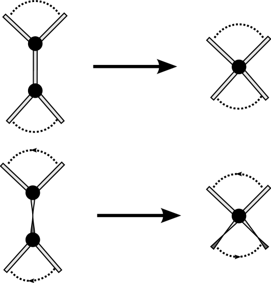
Figure 2. A Möbius graph with two vertices connected by a ribbon may be reduced to a Möbius graph with one less vertex and one less edge. In these graphs the “$\dots$” are to mean that there are arbitrary numbers of other edges at the vertex, and the edges drawn are connected to other vertices. The top graph is an example of this reduction when the connecting ribbon is untwisted, in this case the two vertices are glued together with no other changes in the ribbons. The bottom graph is an example of this reduction when the connecting ribbon is twisted, in this case the two vertices are glued together and the order and orientation (twisted or untwisted) of the ribbons on one side are reversed.

We wish to show that

(3.3) $$\mathbb{E}(X_{1}X_{2}X_{3}X_{4}\dots X_{2n})=(-2)^{\chi({\Gamma})}4^{n-1}\,,$$

where $\Gamma$ is a one vertex Möbius graph with arrows (half edges) labeled by $X_{k}$. We will do this by induction, there are two cases:

1. $X_{1}=\bar{X}_{j}$ for $1<j\leq 2n$,

   $$\mathbb{E}(X_{1}X_{2}\dots X_{j-1}\bar{X}_{1}X_{j+1}\dots X_{2n}) =\mathbb{E}(X_{1}\bar{X}_{1})\mathbb{E}(\Re(X_{2}\dots X_{j-1})\Re(X_{j+1}\dots X_{2n}))$$

   (3.4) $$=4\mathbb{E}(\Re(X_{2}\dots X_{j-1})\Re(X_{j+1}\dots X_{2n}))\,.$$

   This corresponds to the reduction of the Möbius graph pictured in Figure 3, which splits the single vertex into two vertices. The Euler characteristic becomes $\chi_{2}=2-(n-1)+f_{1}=\chi_{1}+2$. By the induction assumption we find

   $$\mathbb{E}(X_{1}\dots X_{2n})=4\left[4^{(n-1)-2}(-2)^{\chi_{2}}\right]=4^{n-2}(-2)^{\chi_{1}+2}=4^{n-1}(-2)^{\chi_{1}}\,.$$

   

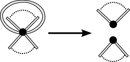
   Figure 3. Here we have an untwisted ribbon of the Möbius graph returning to the same vertex, this edge is removed in our reduction procedure giving us a Möbius graph with one more vertex and one less edge.

2. $X_{1}=X_{j}$ for $1<j\leq 2n$,

   $$\mathbb{E}(X_{1}X_{2}\dots X_{j-1}X_{1}X_{j+1}\dots X_{2n}) =\mathbb{E}(X_{1}X_{1})\mathbb{E}(\bar{X}_{j-1}\dots\bar{X}_{2}X_{j+1}\dots X_{2n})$$

   (3.5) $$=(-2)\mathbb{E}(\bar{X}_{j-1}\dots\bar{X}_{2}X_{j+1}\dots X_{2n})\,.$$

   This corresponds to the reduction of the Möbius graph pictured in Figure 4, which keeps the single vertex and flips the order and orientation of the edges between $X_{1}$ and $X_{j}$. The Euler characteristic becomes $\chi_{2}=1-(n-1)+f_{1}=\chi_{1}+1$. By the induction assumption we find

   $$\mathbb{E}(X_{1}\dots X_{2n})=(-2)\left[4^{(n-1)-1}(-2)^{\chi_{2}}\right]=(-2)^{-1}4^{n-1}(-2)^{\chi_{1}+1}=4^{n-1}(-2)^{\chi_{1}}\,.$$

   

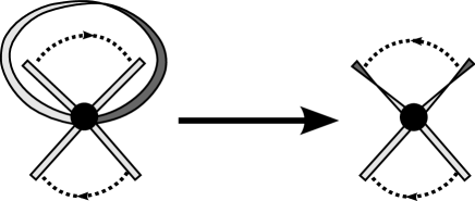
   Figure 4. Here we have a twisted ribbon of the Möbius graph returning to the same vertex, this edge is removed in our reduction procedure giving us a Möbius graph with one less edge and giving a reverse in both the order and orientation (twisted or untwisted) of the ribbons on one side of the removed ribbon.

Note that taking away an oriented ribbon creates a new vertex. The remaining graph might still be connected, or it may split into two components. If taking away a loop makes the graph disconnected, then the counts of changes to edges and vertices are still the same. But the faces need to be counted as follows: the inner face of the removed edge becomes the outside face of one component, and the outer face at the removed edge becomes the outer face of the other component. Thus the counting of faces is not affected by whether the graph is connected.

With these two cases checked, by the induction hypothesis, the proof is completed.

∎

3.3. Bipartite Möbius graphs and quaternionic Gaussian moments

To deal with quaternionic Wishart random matrices, we need to consider a special subclass of quaternionic Gaussian variables from Theorem 3.1. Suppose the $2n$-tuple $(X_{\pm 1},X_{\pm 2},\dots,X_{\pm n})$ consists of $n$ pairs of random variables taken with repetition, from the set $\{Z_{1},Z_{2},\dots,Z_{n}\}$ of independent quaternionic Gaussian random variables. Note that in contrast to the setup for Theorem 3.1, here all $Z$’s are without conjugation. Fix a sequence $j_{1},j_{2},\dots,j_{m}$ of natural numbers such that $j_{1}+\dots+j_{m}=n$. Theorem 3.1 then says that

$$\mathbb{E}\big{(}\Re(\bar{X}_{-1}X_{1}\cdots\bar{X}_{-j_{1}}X_{j_{1}})\times\Re(\bar{X}_{-j_{1}-1}X_{j_{1}+1}\cdots\bar{X}_{-j_{1}-j_{2}}X_{j_{1}+j_{2}})\times\cdots$$

$$\dots\times\Re(\bar{X}_{-j_{1}-j_{2}-\dots-j_{m-1}-1}\cdots\bar{X}_{-n}X_{n})\big{)}$$

$$=4^{n-m}(-2)^{\chi(\Gamma)},$$

where $\Gamma$ is the Möbius graph with $m$ vertices and with edges labeled by $X_{\pm 1},\dots,X_{\pm n}$ that describes the pairings between the variables under the expectation. Our goal is to show that the same formula holds true for another graph, a bipartite Möbius graph whose edges are labeled by $n$ pairs $(X_{-j},X_{j})$, $1\leq j\leq n$.

The bipartite Möbius graph has two types of vertices: black vertices and white (or later, colored) vertices with ribbons that can only connect a black vertex to a white vertex. (As previously, the ribbons may carry a “flip” of orientation which we represent graphically as a twist.) To define this graph, we need to introduce three pair partitions on the set $\{\pm 1,\dots,\pm n\}$. The first partition, $\delta$, pairs $j$ with $-j$. The second partition, $\sigma$, describes the placement of $\Re$: its pairs are

$$\{1,-2\},\{2,-3\},\dots,\{j_{1},-1\},$$

$$\{j_{1}+1,-(j_{1}+2)\},\dots,\{j_{1}+j_{2},-(j_{1}+1)\},$$

$$\vdots$$

$$\{1+\sum_{k=1}^{m-1}j_{k},-(2+\sum_{k=1}^{m-1}j_{k})\},\dots,\{n,-(1+\sum_{k=1}^{m-1}j_{k})\}.$$

The third partition, $\gamma$, describes the choices of pairs from $Z_{1},\dots,Z_{n}$. Thus $\{j,k\}\in\gamma$ if $X_{j}=X_{k}$ when $jk>0$ or $X_{j}=\bar{X}_{k}$ if $jk<0$.

We will also represent these pair partitions as graphs with vertices arranged in two rows, and with the edges drawn between the vertices in each pair of a partition. Thus

(3.6) $$\delta=\begin{matrix}\lx@xy@svg{\hbox{\raise 0.0pt\hbox{\kern 6.10716pt\hbox{\ignorespaces\ignorespaces\ignorespaces\hbox{\vtop{\kern 0.0pt\offinterlineskip\halign{\entry@#!@&&\entry@@#!@\cr&&&\\&&&\\}}}\ignorespaces{\hbox{\kern-4.4pt\raise 0.0pt\hbox{\hbox{\kern 0.0pt\raise 0.0pt\hbox{\hbox{\kern 3.0pt\raise 0.0pt\hbox{$\textstyle{{{}^{1}_{\bullet}}\ignorespaces\ignorespaces\ignorespaces\ignorespaces}$}}}}}}}\ignorespaces\ignorespaces\ignorespaces\ignorespaces{}{\hbox{\lx@xy@droprule}}\ignorespaces{}{\hbox{\lx@xy@droprule}}{\hbox{\lx@xy@droprule}}{\hbox{\kern 19.81433pt\raise 0.0pt\hbox{\hbox{\kern 0.0pt\raise 0.0pt\hbox{\hbox{\kern 3.0pt\raise 0.0pt\hbox{$\textstyle{{{}^{2}_{\bullet}}\ignorespaces\ignorespaces\ignorespaces\ignorespaces}$}}}}}}}\ignorespaces\ignorespaces\ignorespaces\ignorespaces{}{\hbox{\lx@xy@droprule}}\ignorespaces{}{\hbox{\lx@xy@droprule}}{\hbox{\lx@xy@droprule}}{\hbox{\kern 42.32149pt\raise 0.0pt\hbox{\hbox{\kern 0.0pt\raise 0.0pt\hbox{\hbox{\kern 3.0pt\raise 0.0pt\hbox{$\textstyle{\dots}$}}}}}}}{\hbox{\kern 69.248pt\raise 0.0pt\hbox{\hbox{\kern 0.0pt\raise 0.0pt\hbox{\hbox{\kern 3.0pt\raise 0.0pt\hbox{$\textstyle{{{}^{n}_{\bullet}}\ignorespaces\ignorespaces\ignorespaces\ignorespaces}$}}}}}}}\ignorespaces\ignorespaces\ignorespaces\ignorespaces{}{\hbox{\lx@xy@droprule}}\ignorespaces{}{\hbox{\lx@xy@droprule}}{\hbox{\lx@xy@droprule}}{\hbox{\kern-6.10716pt\raise-28.52444pt\hbox{\hbox{\kern 0.0pt\raise 0.0pt\hbox{\hbox{\kern 3.0pt\raise 0.0pt\hbox{$\textstyle{{{}^{\hskip 4.2679pt\bullet}_{-1}}}$}}}}}}}{\hbox{\kern 18.10716pt\raise-28.52444pt\hbox{\hbox{\kern 0.0pt\raise 0.0pt\hbox{\hbox{\kern 3.0pt\raise 0.0pt\hbox{$\textstyle{{{}^{\hskip 4.2679pt\bullet}_{-2}}}$}}}}}}}{\hbox{\kern 42.32149pt\raise-28.52444pt\hbox{\hbox{\kern 0.0pt\raise 0.0pt\hbox{\hbox{\kern 3.0pt\raise 0.0pt\hbox{$\textstyle{\dots}$}}}}}}}{\hbox{\kern 67.82149pt\raise-28.52444pt\hbox{\hbox{\kern 0.0pt\raise 0.0pt\hbox{\hbox{\kern 3.0pt\raise 0.0pt\hbox{$\textstyle{{{}^{\hskip 4.2679pt\bullet}_{-n}}}$}}}}}}}\ignorespaces}}}}\ignorespaces\end{matrix} \textstyle{{{}^{1}_{\bullet}}\ignorespaces\ignorespaces\ignorespaces\ignorespaces} \textstyle{{{}^{2}_{\bullet}}\ignorespaces\ignorespaces\ignorespaces\ignorespaces} \textstyle{\dots} \textstyle{{{}^{n}_{\bullet}}\ignorespaces\ignorespaces\ignorespaces\ignorespaces} \textstyle{{{}^{\hskip 4.2679pt\bullet}_{-1}}} \textstyle{{{}^{\hskip 4.2679pt\bullet}_{-2}}} \textstyle{\dots} \textstyle{{{}^{\hskip 4.2679pt\bullet}_{-n}}} \textstyle{{{}^{1}_{\bullet}}\ignorespaces\ignorespaces\ignorespaces\ignorespaces} \textstyle{{{}^{2}_{\bullet}}\ignorespaces\ignorespaces\ignorespaces\ignorespaces} \textstyle{\dots} \textstyle{{{}^{n}_{\bullet}}\ignorespaces\ignorespaces\ignorespaces\ignorespaces} \textstyle{{{}^{\hskip 4.2679pt\bullet}_{-1}}} \textstyle{{{}^{\hskip 4.2679pt\bullet}_{-2}}} \textstyle{\dots} \textstyle{{{}^{\hskip 4.2679pt\bullet}_{-n}}}$$

and

$$\sigma=\begin{matrix}\lx@xy@svg{\hbox{\raise 0.0pt\hbox{\kern 5.96716pt\hbox{\ignorespaces\ignorespaces\ignorespaces\hbox{\vtop{\kern 0.0pt\offinterlineskip\halign{\entry@#!@&&\entry@@#!@\cr&&&&&&&&&&\\&&&&&&&&&&\crcr}}}\ignorespaces{\hbox{\kern-4.26pt\raise 0.0pt\hbox{\hbox{\kern 0.0pt\raise 0.0pt\hbox{\hbox{\kern 3.0pt\raise 0.0pt\hbox{$\textstyle{{{}^{1}_{\bullet}}\ignorespaces\ignorespaces\ignorespaces\ignorespaces}$}}}}}}}\ignorespaces\ignorespaces\ignorespaces{}\ignorespaces\ignorespaces{\hbox{\lx@xy@drawline@}}\ignorespaces{}\ignorespaces\ignorespaces{\hbox{\lx@xy@drawline@}}\ignorespaces{\hbox{\lx@xy@drawline@}}{\hbox{\kern 19.67433pt\raise 0.0pt\hbox{\hbox{\kern 0.0pt\raise 0.0pt\hbox{\hbox{\kern 3.0pt\raise 0.0pt\hbox{$\textstyle{{{}^{2}_{\bullet}}\ignorespaces\ignorespaces\ignorespaces\ignorespaces}$}}}}}}}\ignorespaces\ignorespaces\ignorespaces{}\ignorespaces\ignorespaces{\hbox{\lx@xy@drawline@}}\ignorespaces{}\ignorespaces\ignorespaces{\hbox{\lx@xy@drawline@}}\ignorespaces{\hbox{\lx@xy@drawline@}}{\hbox{\kern 43.60866pt\raise 0.0pt\hbox{\hbox{\kern 0.0pt\raise 0.0pt\hbox{\hbox{\kern 3.0pt\raise 0.0pt\hbox{$\textstyle{{{}^{3}_{\bullet}}}$}}}}}}}{\hbox{\kern 65.83582pt\raise 0.0pt\hbox{\hbox{\kern 0.0pt\raise 0.0pt\hbox{\hbox{\kern 3.0pt\raise 0.0pt\hbox{$\textstyle{\dots}$}}}}}}}{\hbox{\kern 90.58582pt\raise 0.0pt\hbox{\hbox{\kern 0.0pt\raise 0.0pt\hbox{\hbox{\kern 3.0pt\raise 0.0pt\hbox{$\textstyle{{{}^{j_{1}}_{\bullet}}\ignorespaces\ignorespaces\ignorespaces\ignorespaces}$}}}}}}}\ignorespaces\ignorespaces\ignorespaces{}\ignorespaces\ignorespaces{\hbox{\lx@xy@drawline@}}\ignorespaces{}\ignorespaces\ignorespaces{\hbox{\lx@xy@drawline@}}\ignorespaces{\hbox{\lx@xy@drawline@}}{\hbox{\kern 112.3898pt\raise 0.0pt\hbox{\hbox{\kern 0.0pt\raise 0.0pt\hbox{\hbox{\kern 3.0pt\raise 0.0pt\hbox{$\textstyle{{{}^{j_{1}+1}_{\hskip 7.11317pt\bullet}}\ignorespaces\ignorespaces\ignorespaces\ignorespaces}$}}}}}}}\ignorespaces\ignorespaces\ignorespaces{}\ignorespaces\ignorespaces{\hbox{\lx@xy@drawline@}}\ignorespaces{}\ignorespaces\ignorespaces{\hbox{\lx@xy@drawline@}}\ignorespaces{\hbox{\lx@xy@drawline@}}{\hbox{\kern 140.63382pt\raise 0.0pt\hbox{\hbox{\kern 0.0pt\raise 0.0pt\hbox{\hbox{\kern 3.0pt\raise 0.0pt\hbox{$\textstyle{{}^{j_{1}+2}_{\hskip 8.53581pt\bullet}}$}}}}}}}{\hbox{\kern 168.87784pt\raise 0.0pt\hbox{\hbox{\kern 0.0pt\raise 0.0pt\hbox{\hbox{\kern 3.0pt\raise 0.0pt\hbox{$\textstyle{\dots}$}}}}}}}{\hbox{\kern 193.62784pt\raise 0.0pt\hbox{\hbox{\kern 0.0pt\raise 0.0pt\hbox{\hbox{\kern 3.0pt\raise 0.0pt\hbox{$\textstyle{{{}^{j_{1}+j_{2}}_{\hskip 10.5275pt\bullet}}\ignorespaces\ignorespaces\ignorespaces\ignorespaces}$}}}}}}}\ignorespaces\ignorespaces\ignorespaces{}\ignorespaces\ignorespaces{\hbox{\lx@xy@drawline@}}\ignorespaces{}\ignorespaces\ignorespaces{\hbox{\lx@xy@drawline@}}\ignorespaces{\hbox{\lx@xy@drawline@}}{\hbox{\kern 223.15585pt\raise 0.0pt\hbox{\hbox{\kern 0.0pt\raise 0.0pt\hbox{\hbox{\kern 3.0pt\raise 0.0pt\hbox{$\textstyle{{}^{j_{1}+j_{2}+1}_{\hskip 14.22636pt\bullet}}$}}}}}}}{\hbox{\kern 259.12387pt\raise 0.0pt\hbox{\hbox{\kern 0.0pt\raise 0.0pt\hbox{\hbox{\kern 3.0pt\raise 0.0pt\hbox{$\textstyle{\dots}$}}}}}}}{\hbox{\kern-5.96716pt\raise-27.49098pt\hbox{\hbox{\kern 0.0pt\raise 0.0pt\hbox{\hbox{\kern 3.0pt\raise 0.0pt\hbox{$\textstyle{{{}^{\hskip 4.2679pt\bullet}_{-1}}}$}}}}}}}{\hbox{\kern 17.96716pt\raise-27.49098pt\hbox{\hbox{\kern 0.0pt\raise 0.0pt\hbox{\hbox{\kern 3.0pt\raise 0.0pt\hbox{$\textstyle{{{}^{\hskip 4.2679pt\bullet}_{-2}}}$}}}}}}}{\hbox{\kern 41.90149pt\raise-27.49098pt\hbox{\hbox{\kern 0.0pt\raise 0.0pt\hbox{\hbox{\kern 3.0pt\raise 0.0pt\hbox{$\textstyle{{}^{\hskip 4.2679pt\bullet}_{-3}}$}}}}}}}{\hbox{\kern 65.83582pt\raise-27.49098pt\hbox{\hbox{\kern 0.0pt\raise 0.0pt\hbox{\hbox{\kern 3.0pt\raise 0.0pt\hbox{$\textstyle{\dots}$}}}}}}}{\hbox{\kern 91.22781pt\raise-27.49098pt\hbox{\hbox{\kern 0.0pt\raise 0.0pt\hbox{\hbox{\kern 3.0pt\raise 0.0pt\hbox{$\textstyle{{}_{\bullet}}$}}}}}}}{\hbox{\kern 116.25182pt\raise-27.49098pt\hbox{\hbox{\kern 0.0pt\raise 0.0pt\hbox{\hbox{\kern 3.0pt\raise 0.0pt\hbox{$\textstyle{{{}_{\bullet}}}$}}}}}}}{\hbox{\kern 144.49583pt\raise-27.49098pt\hbox{\hbox{\kern 0.0pt\raise 0.0pt\hbox{\hbox{\kern 3.0pt\raise 0.0pt\hbox{$\textstyle{{}_{\bullet}}$}}}}}}}{\hbox{\kern 168.87784pt\raise-27.49098pt\hbox{\hbox{\kern 0.0pt\raise 0.0pt\hbox{\hbox{\kern 3.0pt\raise 0.0pt\hbox{$\textstyle{\dots}$}}}}}}}{\hbox{\kern 198.13185pt\raise-27.49098pt\hbox{\hbox{\kern 0.0pt\raise 0.0pt\hbox{\hbox{\kern 3.0pt\raise 0.0pt\hbox{$\textstyle{{}_{\bullet}}$}}}}}}}{\hbox{\kern 230.87987pt\raise-27.49098pt\hbox{\hbox{\kern 0.0pt\raise 0.0pt\hbox{\hbox{\kern 3.0pt\raise 0.0pt\hbox{$\textstyle{{}_{\bullet}}$}}}}}}}{\hbox{\kern 259.12387pt\raise-27.49098pt\hbox{\hbox{\kern 0.0pt\raise 0.0pt\hbox{\hbox{\kern 3.0pt\raise 0.0pt\hbox{$\textstyle{\dots}$}}}}}}}\ignorespaces}}}}\ignorespaces\end{matrix} \textstyle{{{}^{1}_{\bullet}}\ignorespaces\ignorespaces\ignorespaces\ignorespaces} \textstyle{{{}^{2}_{\bullet}}\ignorespaces\ignorespaces\ignorespaces\ignorespaces} \textstyle{{{}^{3}_{\bullet}}} \textstyle{\dots} \textstyle{{{}^{j_{1}}_{\bullet}}\ignorespaces\ignorespaces\ignorespaces\ignorespaces} \textstyle{{{}^{j_{1}+1}_{\hskip 7.11317pt\bullet}}\ignorespaces\ignorespaces\ignorespaces\ignorespaces} \textstyle{{}^{j_{1}+2}_{\hskip 8.53581pt\bullet}} \textstyle{\dots} \textstyle{{{}^{j_{1}+j_{2}}_{\hskip 10.5275pt\bullet}}\ignorespaces\ignorespaces\ignorespaces\ignorespaces} \textstyle{{}^{j_{1}+j_{2}+1}_{\hskip 14.22636pt\bullet}} \textstyle{\dots} \textstyle{{{}^{\hskip 4.2679pt\bullet}_{-1}}} \textstyle{{{}^{\hskip 4.2679pt\bullet}_{-2}}} \textstyle{{}^{\hskip 4.2679pt\bullet}_{-3}} \textstyle{\dots} \textstyle{\dots} \textstyle{\dots} \textstyle{{{}^{1}_{\bullet}}\ignorespaces\ignorespaces\ignorespaces\ignorespaces} \textstyle{{{}^{2}_{\bullet}}\ignorespaces\ignorespaces\ignorespaces\ignorespaces} \textstyle{{{}^{3}_{\bullet}}} \textstyle{\dots} \textstyle{{{}^{j_{1}}_{\bullet}}\ignorespaces\ignorespaces\ignorespaces\ignorespaces} \textstyle{{{}^{j_{1}+1}_{\hskip 7.11317pt\bullet}}\ignorespaces\ignorespaces\ignorespaces\ignorespaces} \textstyle{{}^{j_{1}+2}_{\hskip 8.53581pt\bullet}} \textstyle{\dots} \textstyle{{{}^{j_{1}+j_{2}}_{\hskip 10.5275pt\bullet}}\ignorespaces\ignorespaces\ignorespaces\ignorespaces} \textstyle{{}^{j_{1}+j_{2}+1}_{\hskip 14.22636pt\bullet}} \textstyle{\dots} \textstyle{{{}^{\hskip 4.2679pt\bullet}_{-1}}} \textstyle{{{}^{\hskip 4.2679pt\bullet}_{-2}}} \textstyle{{}^{\hskip 4.2679pt\bullet}_{-3}} \textstyle{\dots} \textstyle{\dots} \textstyle{\dots}$$

Consider the 2-regular graphs $\delta\cup\gamma$ and $\delta\cup\sigma$. We orient the cycles of these graphs by ordering $(-j,j)$ on the left-most vertical edge of the cycle. For example,

$$\sigma\cup\delta=\begin{matrix}\lx@xy@svg{\hbox{\raise 0.0pt\hbox{\kern 5.96716pt\hbox{\ignorespaces\ignorespaces\ignorespaces\hbox{\vtop{\kern 0.0pt\offinterlineskip\halign{\entry@#!@&&\entry@@#!@\cr&&&&&&&&&&\\&&&&&&&&&&\crcr}}}\ignorespaces{\hbox{\kern-4.26pt\raise 0.0pt\hbox{\hbox{\kern 0.0pt\raise 0.0pt\hbox{\hbox{\kern 3.0pt\raise 0.0pt\hbox{$\textstyle{{{}^{1}_{\bullet}}\ignorespaces\ignorespaces\ignorespaces\ignorespaces}$}}}}}}}\ignorespaces\ignorespaces\ignorespaces{}\ignorespaces\ignorespaces{\hbox{\lx@xy@drawline@}}\ignorespaces{}\ignorespaces\ignorespaces{\hbox{\lx@xy@drawline@}}\ignorespaces{\hbox{\lx@xy@drawline@}}{\hbox{\kern 19.67433pt\raise 0.0pt\hbox{\hbox{\kern 0.0pt\raise 0.0pt\hbox{\hbox{\kern 3.0pt\raise 0.0pt\hbox{$\textstyle{{{}^{2}_{\bullet}}\ignorespaces\ignorespaces\ignorespaces\ignorespaces}$}}}}}}}\ignorespaces\ignorespaces\ignorespaces{}\ignorespaces\ignorespaces{\hbox{\lx@xy@drawline@}}\ignorespaces{}\ignorespaces\ignorespaces{\hbox{\lx@xy@drawline@}}\ignorespaces{\hbox{\lx@xy@drawline@}}{\hbox{\kern 43.60866pt\raise 0.0pt\hbox{\hbox{\kern 0.0pt\raise 0.0pt\hbox{\hbox{\kern 3.0pt\raise 0.0pt\hbox{$\textstyle{{{}^{3}_{\bullet}}}$}}}}}}}{\hbox{\kern 65.83582pt\raise 0.0pt\hbox{\hbox{\kern 0.0pt\raise 0.0pt\hbox{\hbox{\kern 3.0pt\raise 0.0pt\hbox{$\textstyle{\dots}$}}}}}}}{\hbox{\kern 90.58582pt\raise 0.0pt\hbox{\hbox{\kern 0.0pt\raise 0.0pt\hbox{\hbox{\kern 3.0pt\raise 0.0pt\hbox{$\textstyle{{{}^{j_{1}}_{\bullet}}\ignorespaces\ignorespaces\ignorespaces\ignorespaces}$}}}}}}}\ignorespaces\ignorespaces\ignorespaces{}\ignorespaces\ignorespaces{\hbox{\lx@xy@drawline@}}\ignorespaces{}\ignorespaces\ignorespaces{\hbox{\lx@xy@drawline@}}\ignorespaces{\hbox{\lx@xy@drawline@}}{\hbox{\kern 112.3898pt\raise 0.0pt\hbox{\hbox{\kern 0.0pt\raise 0.0pt\hbox{\hbox{\kern 3.0pt\raise 0.0pt\hbox{$\textstyle{{{}^{j_{1}+1}_{\hskip 7.11317pt\bullet}}\ignorespaces\ignorespaces\ignorespaces\ignorespaces}$}}}}}}}\ignorespaces\ignorespaces\ignorespaces{}\ignorespaces\ignorespaces{\hbox{\lx@xy@drawline@}}\ignorespaces{}\ignorespaces\ignorespaces{\hbox{\lx@xy@drawline@}}\ignorespaces{\hbox{\lx@xy@drawline@}}{\hbox{\kern 140.63382pt\raise 0.0pt\hbox{\hbox{\kern 0.0pt\raise 0.0pt\hbox{\hbox{\kern 3.0pt\raise 0.0pt\hbox{$\textstyle{{}^{j_{1}+2}_{\hskip 8.53581pt\bullet}}$}}}}}}}{\hbox{\kern 168.87784pt\raise 0.0pt\hbox{\hbox{\kern 0.0pt\raise 0.0pt\hbox{\hbox{\kern 3.0pt\raise 0.0pt\hbox{$\textstyle{\dots}$}}}}}}}{\hbox{\kern 193.62784pt\raise 0.0pt\hbox{\hbox{\kern 0.0pt\raise 0.0pt\hbox{\hbox{\kern 3.0pt\raise 0.0pt\hbox{$\textstyle{{{}^{j_{1}+j_{2}}_{\hskip 10.5275pt\bullet}}\ignorespaces\ignorespaces\ignorespaces\ignorespaces}$}}}}}}}\ignorespaces\ignorespaces\ignorespaces{}\ignorespaces\ignorespaces{\hbox{\lx@xy@drawline@}}\ignorespaces{}\ignorespaces\ignorespaces{\hbox{\lx@xy@drawline@}}\ignorespaces{\hbox{\lx@xy@drawline@}}{\hbox{\kern 223.15585pt\raise 0.0pt\hbox{\hbox{\kern 0.0pt\raise 0.0pt\hbox{\hbox{\kern 3.0pt\raise 0.0pt\hbox{$\textstyle{{}^{j_{1}+j_{2}+1}_{\hskip 14.22636pt\bullet}}$}}}}}}}{\hbox{\kern 259.12387pt\raise 0.0pt\hbox{\hbox{\kern 0.0pt\raise 0.0pt\hbox{\hbox{\kern 3.0pt\raise 0.0pt\hbox{$\textstyle{\dots}$}}}}}}}{\hbox{\kern-5.96716pt\raise-27.49098pt\hbox{\hbox{\kern 0.0pt\raise 0.0pt\hbox{\hbox{\kern 3.0pt\raise 0.0pt\hbox{$\textstyle{{{}^{\hskip 4.2679pt\bullet}_{-1}}\ignorespaces\ignorespaces\ignorespaces\ignorespaces}$}}}}}}}\ignorespaces\ignorespaces\ignorespaces\ignorespaces{}{\hbox{\lx@xy@droprule}}\ignorespaces{\hbox{\kern 0.0pt\raise-4.12pt\hbox{\hbox{\kern 0.0pt\raise 0.0pt\hbox{\lx@xy@tip{1}\lx@xy@tip{-1}}}}}}{\hbox{\lx@xy@droprule}}{\hbox{\lx@xy@droprule}}{\hbox{\kern 17.96716pt\raise-27.49098pt\hbox{\hbox{\kern 0.0pt\raise 0.0pt\hbox{\hbox{\kern 3.0pt\raise 0.0pt\hbox{$\textstyle{{{}^{\hskip 4.2679pt\bullet}_{-2}}\ignorespaces\ignorespaces\ignorespaces\ignorespaces}$}}}}}}}\ignorespaces\ignorespaces\ignorespaces\ignorespaces{}{\hbox{\lx@xy@droprule}}\ignorespaces{}{\hbox{\lx@xy@droprule}}{\hbox{\lx@xy@droprule}}{\hbox{\kern 41.90149pt\raise-27.49098pt\hbox{\hbox{\kern 0.0pt\raise 0.0pt\hbox{\hbox{\kern 3.0pt\raise 0.0pt\hbox{$\textstyle{{{}^{\hskip 4.2679pt\bullet}_{-3}}\ignorespaces\ignorespaces\ignorespaces\ignorespaces}$}}}}}}}\ignorespaces\ignorespaces\ignorespaces\ignorespaces{}{\hbox{\lx@xy@droprule}}\ignorespaces{}{\hbox{\lx@xy@droprule}}{\hbox{\lx@xy@droprule}}{\hbox{\kern 65.83582pt\raise-27.49098pt\hbox{\hbox{\kern 0.0pt\raise 0.0pt\hbox{\hbox{\kern 3.0pt\raise 0.0pt\hbox{$\textstyle{\dots}$}}}}}}}{\hbox{\kern 91.22781pt\raise-27.49098pt\hbox{\hbox{\kern 0.0pt\raise 0.0pt\hbox{\hbox{\kern 3.0pt\raise 0.0pt\hbox{$\textstyle{{{}_{\bullet}}\ignorespaces\ignorespaces\ignorespaces\ignorespaces}$}}}}}}}\ignorespaces\ignorespaces\ignorespaces\ignorespaces{}{\hbox{\lx@xy@droprule}}\ignorespaces{}{\hbox{\lx@xy@droprule}}{\hbox{\lx@xy@droprule}}{\hbox{\kern 116.25182pt\raise-27.49098pt\hbox{\hbox{\kern 0.0pt\raise 0.0pt\hbox{\hbox{\kern 3.0pt\raise 0.0pt\hbox{$\textstyle{{{}_{\bullet}}\ignorespaces\ignorespaces\ignorespaces\ignorespaces}$}}}}}}}\ignorespaces\ignorespaces\ignorespaces\ignorespaces{}{\hbox{\lx@xy@droprule}}\ignorespaces{\hbox{\kern 120.51181pt\raise-4.12pt\hbox{\hbox{\kern 0.0pt\raise 0.0pt\hbox{\lx@xy@tip{1}\lx@xy@tip{-1}}}}}}{\hbox{\lx@xy@droprule}}{\hbox{\lx@xy@droprule}}{\hbox{\kern 144.49583pt\raise-27.49098pt\hbox{\hbox{\kern 0.0pt\raise 0.0pt\hbox{\hbox{\kern 3.0pt\raise 0.0pt\hbox{$\textstyle{{{}_{\bullet}}\ignorespaces\ignorespaces\ignorespaces\ignorespaces}$}}}}}}}\ignorespaces\ignorespaces\ignorespaces\ignorespaces{}{\hbox{\lx@xy@droprule}}\ignorespaces{}{\hbox{\lx@xy@droprule}}{\hbox{\lx@xy@droprule}}{\hbox{\kern 168.87784pt\raise-27.49098pt\hbox{\hbox{\kern 0.0pt\raise 0.0pt\hbox{\hbox{\kern 3.0pt\raise 0.0pt\hbox{$\textstyle{\dots}$}}}}}}}{\hbox{\kern 198.13185pt\raise-27.49098pt\hbox{\hbox{\kern 0.0pt\raise 0.0pt\hbox{\hbox{\kern 3.0pt\raise 0.0pt\hbox{$\textstyle{{{}_{\bullet}}\ignorespaces\ignorespaces\ignorespaces\ignorespaces}$}}}}}}}\ignorespaces\ignorespaces\ignorespaces\ignorespaces{}{\hbox{\lx@xy@droprule}}\ignorespaces{}{\hbox{\lx@xy@droprule}}{\hbox{\lx@xy@droprule}}{\hbox{\kern 230.87987pt\raise-27.49098pt\hbox{\hbox{\kern 0.0pt\raise 0.0pt\hbox{\hbox{\kern 3.0pt\raise 0.0pt\hbox{$\textstyle{{{}_{\bullet}}\ignorespaces\ignorespaces\ignorespaces\ignorespaces}$}}}}}}}\ignorespaces\ignorespaces\ignorespaces\ignorespaces{}{\hbox{\lx@xy@droprule}}\ignorespaces{\hbox{\kern 235.13986pt\raise-4.12pt\hbox{\hbox{\kern 0.0pt\raise 0.0pt\hbox{\lx@xy@tip{1}\lx@xy@tip{-1}}}}}}{\hbox{\lx@xy@droprule}}{\hbox{\lx@xy@droprule}}{\hbox{\kern 259.12387pt\raise-27.49098pt\hbox{\hbox{\kern 0.0pt\raise 0.0pt\hbox{\hbox{\kern 3.0pt\raise 0.0pt\hbox{$\textstyle{\dots}$}}}}}}}\ignorespaces}}}}\ignorespaces\end{matrix} \textstyle{{{}^{1}_{\bullet}}\ignorespaces\ignorespaces\ignorespaces\ignorespaces} \textstyle{{{}^{2}_{\bullet}}\ignorespaces\ignorespaces\ignorespaces\ignorespaces} \textstyle{{{}^{3}_{\bullet}}} \textstyle{\dots} \textstyle{{{}^{j_{1}}_{\bullet}}\ignorespaces\ignorespaces\ignorespaces\ignorespaces} \textstyle{{{}^{j_{1}+1}_{\hskip 7.11317pt\bullet}}\ignorespaces\ignorespaces\ignorespaces\ignorespaces} \textstyle{{}^{j_{1}+2}_{\hskip 8.53581pt\bullet}} \textstyle{\dots} \textstyle{{{}^{j_{1}+j_{2}}_{\hskip 10.5275pt\bullet}}\ignorespaces\ignorespaces\ignorespaces\ignorespaces} \textstyle{{}^{j_{1}+j_{2}+1}_{\hskip 14.22636pt\bullet}} \textstyle{\dots} \textstyle{{{}^{\hskip 4.2679pt\bullet}_{-1}}\ignorespaces\ignorespaces\ignorespaces\ignorespaces} \textstyle{{{}^{\hskip 4.2679pt\bullet}_{-2}}\ignorespaces\ignorespaces\ignorespaces\ignorespaces} \textstyle{{{}^{\hskip 4.2679pt\bullet}_{-3}}\ignorespaces\ignorespaces\ignorespaces\ignorespaces} \textstyle{\dots} \textstyle{\dots} \textstyle{\dots} \textstyle{{{}^{1}_{\bullet}}\ignorespaces\ignorespaces\ignorespaces\ignorespaces} \textstyle{{{}^{2}_{\bullet}}\ignorespaces\ignorespaces\ignorespaces\ignorespaces} \textstyle{{{}^{3}_{\bullet}}} \textstyle{\dots} \textstyle{{{}^{j_{1}}_{\bullet}}\ignorespaces\ignorespaces\ignorespaces\ignorespaces} \textstyle{{{}^{j_{1}+1}_{\hskip 7.11317pt\bullet}}\ignorespaces\ignorespaces\ignorespaces\ignorespaces} \textstyle{{}^{j_{1}+2}_{\hskip 8.53581pt\bullet}} \textstyle{\dots} \textstyle{{{}^{j_{1}+j_{2}}_{\hskip 10.5275pt\bullet}}\ignorespaces\ignorespaces\ignorespaces\ignorespaces} \textstyle{{}^{j_{1}+j_{2}+1}_{\hskip 14.22636pt\bullet}} \textstyle{\dots} \textstyle{{{}^{\hskip 4.2679pt\bullet}_{-1}}\ignorespaces\ignorespaces\ignorespaces\ignorespaces} \textstyle{{{}^{\hskip 4.2679pt\bullet}_{-2}}\ignorespaces\ignorespaces\ignorespaces\ignorespaces} \textstyle{{{}^{\hskip 4.2679pt\bullet}_{-3}}\ignorespaces\ignorespaces\ignorespaces\ignorespaces} \textstyle{\dots} \textstyle{\dots} \textstyle{\dots}$$

We now define the bipartite Möbius graph by assigning black vertices to the $m$ cycles of $\delta\cup\sigma$, and white vertices to the cycles of $\delta\cup\gamma$.

Each black vertex is oriented counter-clockwise. For each black vertex we follow the cycle of $\delta\cup\sigma$, drawing a labeled line for each element of the partition. The lines corresponding to $-j,j$ are adjacent, and will eventually become two edges of a ribbon.

Each white vertex is oriented, say, clockwise; we identify the graphs that differ only by a choice of orientation at some of the white vertices. For each white vertex, we follow the corresponding cycle of $\delta\cup\gamma$, drawing a labeled line for each element of the partition. The lines corresponding to $-j,j$ are adjacent, but may appear in two different orders depending on the orientation of the corresponding edge of $\delta$ on the cycle.

The final step is to connect pairs $(j,-j)$ on the black vertices with the same pairs on the white vertices. This creates the ribbons, which carry a flip if the orientation of the two lines on the black vertex does not match the orientation of the same edges on the white vertex.

Figure 5. Representation of a bipartite Möbius graph, the edges drawn are ribbons that are either twisted or untwisted.

The individual edges pictured in Figure 5 are ribbons and are labeled as in Figure 6.

Figure 6. Example of the labeling we use for the edges emanating from a black vertex in a bipartite Möbius graph.

We allow twists of ribbons to propagate through a white vertex calling the two bipartite Möbius graphs equivalent.

Suppose the $2n$-tuple $(X_{\pm 1},X_{\pm 2},\dots,X_{\pm n})$ consists of random variables taken with repetition, from the set $\{Z_{1},Z_{2},\dots,Z_{n}\}$ of independent quaternionic Gaussian random variables. Let $\mathcal{M}=\mathcal{M}(X_{\pm 1},X_{\pm 2},\dots,X_{\pm n})$ denote the set of all bipartite Möbius graphs $\Gamma$ that correspond to various ways of pairing all repeated $Z$’s in the sequence $(X_{\pm 1},X_{\pm 2},\dots,X_{\pm n})$; the pairs are given by adjacent half edges at each white vertex. (See the preceding construction.) $\mathcal{M}=\emptyset$ if there is a $Z_{j}$ that is repeated an odd number of times.

Theorem 3.2.

$$\mathbb{E}\big{(}\Re(\bar{X}_{-1}X_{1}\cdots\bar{X}_{-j_{1}}X_{j_{1}})\times\Re(\bar{X}_{-j_{1}-1}X_{j_{1}+1}\cdots\bar{X}_{-j_{1}-j_{2}}X_{j_{1}+j_{2}})\times\cdots$$

$$\dots\times\Re(\bar{X}_{-j_{1}-j_{2}-\dots-j_{m-1}-1}\cdots\bar{X}_{-n}X_{n})\big{)}$$

$$=4^{n-m}\sum_{\Gamma\in\mathcal{M}}(-2)^{\chi(\Gamma)}\;,$$

(The right hand side is interpreted as $0$ when $\mathcal{M}=\emptyset$.)

Proof.

The proof is fundamentally the same as that of the Wigner version of this theorem. In view of (2.9) and (2.10), it suffices to consider $\{X_{\pm 1},\dots X_{\pm n}\}$ that form $n$ independent pairs, and show that

(3.7) $$\mathbb{E}\big{(}\Re(\bar{X}_{-1}X_{1}\cdots\bar{X}_{-j_{1}}X_{j_{1}})\times\Re(\bar{X}_{-j_{1}-1}X_{j_{1}+1}\cdots\bar{X}_{-j_{1}-j_{2}}X_{j_{1}+j_{2}})\times\cdots\\ \dots\times\Re(\bar{X}_{-j_{1}-j_{2}-\dots-j_{m-1}-1}\cdots\bar{X}_{-n}X_{n})\big{)}=4^{n-m}(-2)^{\chi(\Gamma)}\;,$$

where $\Gamma$ is the bipartite Möbius graph that describes the pairings.

We will prove (3.7) by induction; to that end we first check that with $n=1,m=1$ we have $\mathbb{E}(\bar{X}X)=(-2)^{2}$ in agreement with (3.7).

If $\Gamma$ has two black vertices connected together by edges adjacent at a white vertex, we can use the cyclicity of $\Re$ to move the variables that label the respective edges and share the same face to the first position in their cycles, so that we may call them $\bar{X}_{-1}$ and either $X_{j}$ or $\bar{X}_{-j}$. We now use relations (2.6) and (2.7) to eliminate the pair from the product:

$$\mathbb{E}\left(\Re(\bar{X}_{-1}\cdots X_{j_{1}})\Re(X_{j}\dots X_{j_{1}+j_{2}}\bar{X}_{-j})\right)=\mathbb{E}(X_{1}\cdots X_{j_{1}+j_{2}}\bar{X}_{-j})\,,$$

or

$$\mathbb{E}\left(\Re(\bar{X}_{-1}\cdots X_{j_{1}})\Re(\bar{X}_{j}\dots X_{j_{1}+j_{2}})\right)=\mathbb{E}(\bar{X}_{j_{1}}X_{-j_{1}}\cdots\bar{X}_{1}X_{j}\cdots X_{j_{1}+j_{2}})\,.$$

The use of relation (2.6) corresponds to that of gluing together the two ribbons along the halves adjacent at the white vertex, and gluing together the corresponding black vertices (see Figure 7). The use of relation (2.7) corresponds to the same gluing, but in this case one of the ribbons has an orientation reversal in it, resulting in an orientation reversal for the remaining sides (see Figure 8). These geometric operations reduce $n$ and $m$ by one without changing the Euler characteristic: both the number of edges and the number of vertices are reduced by one while the number of faces is preserved.

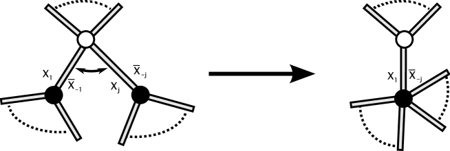
Figure 7. Here two black vertices are connected together through untwisted edges adjacent at a white vertex. This bipartite Möbius graph reduces to one with one less vertex and one less edge. The reduction is found by gluing the two black vertices together and gluing the two ribbons together along their adjacent sides, here labeled by $\bar{X}_{-1}$ and $X_{j}$. The same reduction would apply if the two edges were twisted as we could pass this twist through the white vertex.

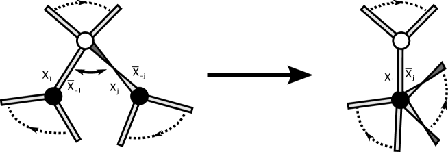
Figure 8. Here two black vertices are connected together through one twisted edge and one untwisted edge adjacent at a white vertex. This bipartite Möbius graph reduces to one with one less vertex and one less edge. The reduction is found by gluing the two black vertices together, gluing the two ribbons together along the sides adjacent at the white vertex, and reversing both the order and orientations of remaining ribbons on the second black vertex.

Therefore we will only need to prove the result for the single black vertex case of the induction step. We wish to show that

(3.8) $$\mathbb{E}(\bar{X}_{-1}X_{1}\bar{X}_{-2}X_{2}\cdots\bar{X}_{-n}X_{n})=4^{n-1}(-2)^{\chi(\Gamma)}\;,$$

where $\Gamma$ is a bipartite Möbius graph with a single black vertex and half ribbons labeled by $X_{\pm k}$. We will do this by induction, there are two cases:

1. $X_{-1}=X_{j}$ for $1\leq j\leq n$,

   $$\mathbb{E}(\bar{X}_{-1}X_{1}\cdots\bar{X}_{-j}X_{j}\cdots X_{n}) =\mathbb{E}(\bar{X}_{-1}X_{j})\mathbb{E}(\Re(X_{1}\cdots\bar{X}_{-j})\Re(\bar{X}_{-j-1}X_{j+1}\cdots X_{n}))$$

   $$=4\mathbb{E}(\Re(\bar{X}_{-j}X_{1}\cdots X_{j-1})\Re(\bar{X}_{-j-1}X_{j+1}\cdots X_{n}))\,.$$

   This corresponds to the reduction of the bipartite Möbius graph pictured in Figure 9, which for $j>1$ splits the single black vertex into two black vertices, and glues the two edges labeled as $\bar{X}_{-1}$ and $X_{j}$ together.

   The edges $(1,-1,j,-j)$ are adjacent at the white vertex and appear either in this order, or in the reverse order. Thus after the removal of $\{-1,j\}$ we get an ordered pair of labels $(1,-j)$ or $(-j,1)$ to glue back into a ribbon. On the black vertex, due to our conventions the edges of the ribbons appear in the following order

   $$((-1,1),(-2,2),\dots,(-j,j),(-k_{1},k_{1}),\dots,(-k_{r},k_{r})).$$

   Once we split the black vertex into two vertices with the edges of ribbons given by $((-1,1),(-2,2),\dots,(-j,j))$ and $((-k_{1},k_{1}),\dots,(-k_{r},k_{r}))$, the removal of $\{-1,j\}$ creates a new pair $(1,-j)$ which we use to create the ribbon to the white vertex. [After this step, we relabel all edges to use again $\pm 1,\pm 2,\dots$ consecutively.]

   We note that the number of faces of the new graph is the same as the previous graph – the face with the sequence of edges

   $$(\dots,X_{k_{r}},\bar{X}_{-1},X_{j},\bar{X}_{-k_{1}},\dots)$$

   becomes the face with edges $(\dots,X_{k_{r}},\bar{X}_{-k_{1}},\dots)$ on the new graph. The Euler characteristic becomes $\chi_{2}=(v_{1}+1)-(e_{1}-1)+f_{1}=\chi_{1}+2$ where $v_{1},e_{1}$ and $f_{1}$ are the number of vertices, edges, and faces of $\Gamma$. By the induction assumption we then find

   $$\mathbb{E}(\bar{X}_{-1}X_{1}\cdots X_{n})=4\left[4^{(n-1)-2}(-2)^{\chi_{2}}\right]=4^{n-2}(-2)^{\chi_{1}+2}=4^{n-1}(-2)^{\chi_{1}}\,.$$

   

   Figure 9. Here we have a black vertex with two ribbons, both twisted or both untwisted, adjacent at the same white vertex. The reduction glues these two ribbons together along their common side. The result is a bipartite Möbius graph with one more vertex and one less edge. The resulting graph may or may not be disconnected at this point.

2. $X_{-1}=X_{-j}$ for $1<j\leq n$,

   $$\mathbb{E}(\bar{X}_{-1}X_{1}\cdots\bar{X}_{-j}X_{j}\cdots X_{n})\\ =\mathbb{E}(\bar{X}_{-1}\bar{X}_{-j})\mathbb{E}(\bar{X}_{j-1}X_{-j+1}\cdots\bar{X}_{1}X_{j}\bar{X}_{-j-1}X_{j+1}\cdots X_{n})\\ =(-2)\mathbb{E}(\bar{X}_{j-1}X_{-j+1}\cdots\bar{X}_{1}X_{j}\bar{X}_{-j-1}X_{j+1}\cdots X_{n})\,.$$

   This corresponds to the reduction of the Möbius graph pictured in Figure 10, which switches the order and the orientations of the ribbons on one side of the black vertex from the $\pm 1$ and $\pm j$ ribbons and glues the two edges adjacent at the white vertex together as shown. As previously, the removed edges are adjacent at the white vertex. At the black vertex, the labeled lines for the construction of the bipartite graph change from the sequence

   $$(-1,1),(-2,2),\dots,(-j+1,j-1),(-j,j),(-k_{1},k_{1}),\dots,(-k_{r},k_{r})$$

   to the sequence

   $$(j-1,-j+1),\dots,(2,-2),(1,j),(-k_{1},k_{1}),\dots,(-k_{r},k_{r})$$

   which then needs to be relabeled to use $\pm 1,\dots,\pm n$. Again the number of faces on the bipartite graphs is preserved: the face with edges

   $$(\dots,2,-1,-j,k_{1},\dots)$$

   becomes the face

   $$(\dots,2,1,j,k_{1},\dots).$$

   The Euler characteristic becomes $\chi_{2}=v_{1}-(e_{1}-1)+f_{1}=\chi_{1}+1$. By the induction assumption we then find

   $$\mathbb{E}(\bar{X}_{-1}X_{1}\cdots X_{n})=(-2)\left[4^{(n-1)-1}(-2)^{\chi_{2}}\right]=(-2)4^{n-2}(-2)^{\chi_{1}+1}=4^{n-1}(-2)^{\chi_{1}}\,.$$

   

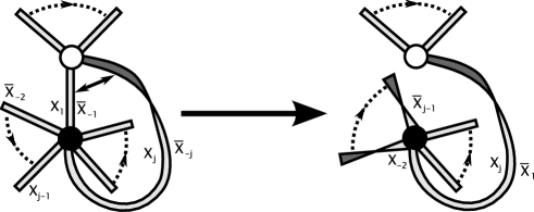
   Figure 10. Here we have a black vertex with two ribbons, one twisted and the other untwisted, adjacent at the same white vertex. The reduction glues these two ribbons together along their common side. The result is a bipartite Möbius graph with one less edge, and with the ribbons on one side of the removed ribbon now with reversed order and orientations.

With these two cases checked, by the induction hypothesis, the proof is completed.

∎

One should note that this is fundamentally the same proof as in the Wigner case, however in this case the geometric reduction is given by gluing together two ribbons, while in the Wigner case the geometric reduction is the elimination of one ribbon at a time. The inductive steps remain the same.

4. Duality between real and symplectic ensembles

By $\mathcal{M}_{M\times N}(\mathbb{H})$ we denote the set of all $M\times N$ matrices with entries from $\mathbb{H}$. For $\mathbf{A}\in\mathcal{M}_{M\times N}(\mathbb{H})$, the adjoint matrix is $A^{*}_{i,j}:=\overline{A}_{j,i}$. The trace is ${\rm tr}(\mathbf{A})=\sum_{j=1}^{N}A_{jj}$. Since the traces ${\rm tr}(\mathbf{A})$ may fail to commute, in the formulas we will use $\Re({\rm tr}(\mathbf{A}))$, compare to [10].

4.1. Duality between GOE and GSE ensembles

The Gaussian orthogonal ensembles consist of square symmetric matrices, $\mathbf{Z}$, whose independent entries are independent (real) Gaussian random variables; the off diagonal entries have variance $1$ while the diagonal entries have variance $2$. One may show that

Theorem B.

For $\mathbf{Z}$ from the $N\times N$ Gaussian orthogonal ensemble:

$$\frac{1}{N^{n-m}}\mathbb{E}({\rm tr}(\mathbf{Z}^{j_{1}}){\rm tr}(\mathbf{Z}^{j_{2}})\dots\rm tr(\mathbf{Z}^{j_{m}}))=\sum_{\Gamma}N^{\chi(\Gamma)}\,,$$

where the sum is over labeled Möbius graphs $\Gamma$ with $m$ vertices of degree $j_{1},j_{2},\dots,j_{m}$, $\chi(\Gamma)$ is the Euler characteristic and $j_{1}+j_{2}+\dots+j_{m}=2n$. More generally, if $\mathbf{Z}_{1},\dots,\mathbf{Z}_{s}$ are independent $N\times N$ GOE ensembles and $t:\{1,2,\dots,2n\}\to\{1,\dots,s\}$ is fixed, then

$$\frac{1}{N^{n-m}}\mathbb{E}({\rm tr}(\mathbf{Z}_{t(1)}\dots\mathbf{Z}_{t(\beta_{1})}){\rm tr}(\mathbf{Z}_{t(\alpha_{2})}\dots\mathbf{Z}_{t(\beta_{2})})\times\dots{\\ }\dots\times{\rm tr}(\mathbf{Z}_{t(\alpha_{m})}\dots\mathbf{Z}_{t(\beta_{m})}))=\sum_{\Gamma}N^{\chi(\Gamma)}\,,$$

where $\alpha_{1}=1$, $\alpha_{k}=j_{1}+j_{2}+\dots+j_{k-1}+1$, and $\beta_{k}=j_{1}+j_{2}+\dots+j_{k}$ denote the ranges under the traces, and where the sum is over labeled color-preserving Möbius graphs $\Gamma$ with vertices of degree $j_{1},j_{2},\dots,j_{m}$ whose edges are colored by the mapping $t$. If there are no $\Gamma$ that are consistent with the coloring we interpret the sum as being $0$.

The single color version of this Theorem was given in Ref. [8].

The Gaussian symplectic ensembles (GSE) consist of square self-adjoint matrices

(4.1) $$\mathbf{Z}=\left[Z_{i,j}\right],$$

where $\{Z_{i,j}:i<j\}$ is a family of independent $\mathbb{H}$-Gaussian random variables (2.3), $\{Z_{i,i}\}$ is a family of independent real Gaussian random variables of variance $2$, and $Z_{i,j}=\bar{Z}_{j,i}$. The law of such a matrix has a density $C\exp(-\frac{1}{4}\Re{\rm tr}(\mathbf{x}^{2}))$, which is supported on the self-adjoint subset of $\mathcal{M}_{N\times N}(\mathbb{H})$. ($C=C(N)$ is a normalizing constant.)

In this section we will demonstrate a multi-matrix version of the theorem of Mulase and Waldron [21] from our Wick formula. This represents an improvement to the argument of Mulase and Waldron as we will not need to rely on labelings of the vertices by the quaternions $1,i,j,$ and $k$. This part of their argument is encoded in relations (2.4-2.7).

We will compute here the expected values of the real traces of powers of a quaternionic self-dual matrix in the Gaussian symplectic ensemble (4.1) where the off-diagonal matrix entries are (2.3).

The basic theorem we will prove is

Theorem 4.1.

For $\mathbf{Z}$ from the $N\times N$ Gaussian symplectic ensemble:

(4.2) $$\frac{1}{(4N)^{n-m}}\mathbb{E}(\Re({\rm tr}(\mathbf{Z}^{j_{1}}))\Re({\rm tr}(\mathbf{Z}^{j_{2}}))\dots\Re({\rm tr}(\mathbf{Z}^{j_{m}})))=\sum_{\Gamma}(-2N)^{\chi(\Gamma)}\,,$$

where the sum is over labeled Möbius graphs $\Gamma$ with $m$ vertices of degree $j_{1},j_{2},\dots,j_{m}$, $\chi(\Gamma)$ is the Euler characteristic and $j_{1}+j_{2}+\dots+j_{m}=2n$.

More generally, suppose $\mathbf{Z}_{1},\dots,\mathbf{Z}_{s}$ are independent $N\times N$ $GSE$ ensembles and $t:\{1,\dots,2n\}\to\{1,\dots,s\}$ is fixed. Let $\alpha_{1}=1$, $\alpha_{k}=j_{1}+j_{2}+\dots+j_{k-1}+1$, $\beta_{k}=j_{1}+j_{2}+\dots+j_{k}$ denote the ranges under traces. Then

(4.3) $$\frac{1}{(4N)^{n-m}}\mathbb{E}\big{(}\Re({\rm tr}(\mathbf{Z}_{t(1)}\dots\mathbf{Z}_{t(\beta_{1})}))\Re({\rm tr}(\mathbf{Z}_{t(\alpha_{2})}\dots\mathbf{Z}_{t(\beta_{2})}))\times\dots{\\ }\dots\times\Re({\rm tr}(\mathbf{Z}_{t(\alpha_{m})}\dots\mathbf{Z}_{t(\beta_{m})}))\big{)}=\sum_{\Gamma}(-2N)^{\chi(\Gamma)}\,,$$

where the sum is over labeled color-preserving Möbius graphs $\Gamma$ with vertices of degree $j_{1}$, $j_{2}$, $\dots$, $j_{m}$ that are colored with $s$ colors by the mapping $t$. As previously, $\chi(\Gamma)$ is the Euler characteristic and $j_{1}+j_{2}+\dots+j_{m}=2n$. (If there are no $\Gamma$ that are consistent with the coloring $t$, we interpret the sum as $0$.)

In view of Theorem B, Theorem 4.1 gives the duality between the GOE and GSE ensembles of random matrices as $N\to-2N$.

Example 4.1.

To illustrate the multi-matrix aspect of the theorem, suppose $\mathbf{Z}_{1},\mathbf{Z}_{2}$ are independent $N\times N$ GSE ensembles and $\mathbf{X}_{1},\mathbf{X}_{2}$ are independent $N\times N$ GOE ensembles. For $p,r,k\geq 0$ let $b_{p,r,k}(N):=\mathbb{E}(({\rm tr}(\mathbf{X}_{1}^{2p}\mathbf{X}_{2}^{2r}))^{k})$. By Theorem B, $b_{p,r,k}(N)=N^{(p+r-1)k}\sum_{\Gamma}N^{\chi(\Gamma)}$. Therefore Theorem 4.1 implies that the moments for the independent GSE ensembles are determined from the corresponding moments of independent GOE ensembles by the “dual formula”

$$\mathbb{E}(({\rm tr}(\mathbf{Z}_{1}^{2p}\mathbf{Z}_{2}^{2r}))^{k})=(-2)^{(p+r-1)k}b_{p,r,k}(-2N).$$

In particular,

$$\mathbb{E}({\rm tr}(\mathbf{Z}_{1}^{2p}))=(-2)^{p-1}b_{p,0,1}(N).$$

This is equivalent to [17, Theorem 6] with $c_{p}(N)=\mathbb{E}({\rm tr}(\mathbf{Z}^{2p}))/2^{p}$; an extra factor of $2^{p}$ in our formula is due to the fact that the symplectic ensemble in [17] has the variance of $1/2$ instead of our choice of $1$.

Proof of Theorem 4.1.

We begin by expanding out the traces in terms of the matrix entries

(4.4) $$\frac{N^{m}}{4^{n-m}}\mathbb{E}(\Re({\rm tr}(\mathbf{Z}^{j_{1}}))\Re({\rm tr}(\mathbf{Z}^{j_{2}}))\dots\Re({\rm tr}(\mathbf{Z}^{j_{m}})))=$$

$$= \sum_{\begin{matrix}1\leq a_{1},a_{2},\dots,a_{j_{1}}\leq N\\ 1\leq b_{1},b_{2},\dots,b_{j_{2}}\leq N\\ \vdots\\ 1\leq c_{1},c_{2},\dots,c_{j_{m}}\leq N\end{matrix}}\begin{matrix}\frac{1}{(4n)^{n-m}}\mathbb{E}(\Re(Z_{a_{1},a_{2}}Z_{a_{2},a_{3}}\dots Z_{a_{j_{1}},a_{1}})\Re(Z_{b_{1},b_{2}}\dots Z_{b_{j_{2}},b_{1}})\times\dots\\ \hfill\dots\times\Re(Z_{c_{1},c_{2}}\dots Z_{c_{j_{m}},c_{1}}))\,.\end{matrix}$$

Note that essentially the same expansion applies to (4.3), except that the consecutive entries $Z_{i,j}^{(t)}$ must now be labeled also by the “color” $t$. It is then better to index the products by the cycles of a permutation. Put

$$\sigma=(1,\dots,\beta_{1})(\alpha_{2},\dots,\beta_{2})\ldots(\alpha_{m},\dots,2n)\,.$$

In this notation, the expansion of the left hand side of (4.3) takes the form

$$\sum_{a:\{1\dots 2n\}\to\{1\dots N\}}\mathbb{E}\left(\prod_{c\in\sigma}\Re(\prod_{j\in c}[\mathbf{Z}_{t(j)}]_{a(j),a(\sigma(j))})\right).$$

(Since $\Re$ has the cyclic property 2.2, this expression is well defined.)

From (2.10) it follows that the right hand side of (4.4) can be expanded as a sum over all pairings, and we can assume that the pairs are independent.

Of course, pairings that match two independent random variables do not contribute to the sum. The pairings that contribute to the sum are of three different types: pairs that match $Z$ with another $Z$ at a different position in the product, pairs that match $Z$ with $\bar{Z}$, and pairings that match the diagonal (real) entries.

We first dispense with the pairings that match a diagonal entry $Z_{i,i}=\xi$ with another diagonal entry $Z_{j,j}=\xi$. Since real numbers commute with quaternions,

$$\Re(\mathbb{E}(q_{0}\xi q_{1}\xi q_{2}))=\mathbb{E}(\xi^{2})\Re(q_{0}q_{1}q_{2})=2\Re(q_{0}q_{1}q_{2}).$$

On the other hand, using the cyclic property of $\Re(\cdot)$ and adding formulas (2.4) and (2.5), we see that the same answer arises from

$$\mathbb{E}\Re(q_{0}Zq_{1}Zq_{2})+\mathbb{E}\Re(q_{0}Zq_{1}\bar{Z}q_{2})=\mathbb{E}\Re(Zq_{1}Zq_{2}q_{0})+\mathbb{E}\Re(Zq_{1}\bar{Z}q_{2}q_{0})=2\Re(q_{1}q_{2}q_{0}).$$

So the contribution of each such diagonal pairing is the same as that of two matches of quaternionic entries $(Z,Z)$ and $(Z,\bar{Z})$.

Thus, once we replace all the real entries that came from the diagonal entries by the corresponding quaternion-Gaussian pairs, we get the sum over all possible pairs of matches of the first two types only. We label all such pairings by Möbius graphs, with the interpretation that pairings or random variables $(Z,Z)$ correspond to twisted ribbons, while pairings $(Z,\bar{Z})$ correspond to ribbons without a twist. The pairs of variables at different ribbons can now be assumed independent. In the multi-matrix case, the edges of the graph at each vertex are colored according to the function $t$, which restricts the number of available pairings.

We now relabel the $Z_{i,j}$ by $Z_{a_{k},a_{k+1}}=X_{k}$, $Z_{b_{k},b_{k+1}}=X_{j_{1}+k}$, $\dots$, $Z_{c_{k},c_{k+1}}=X_{j_{1}+j_{2}+\dots j_{m-1}+k}$. Our claim is then that given a Möbius graph $\Gamma$ with vertices of degree $j_{1}$, $j_{2},\dots,$ and $j_{m}$ with edges labeled by $X_{k}$, satisfies

(4.5) $$\frac{1}{(4N)^{n-m}}\mathbb{E}(\Re(X_{1}\dots X_{j_{1}})\Re(X_{j_{1}+1}\dots X_{j_{1}+j_{2}})\dots\Re(X_{j_{1}+\dots+j_{m-1}+1}\dots X_{2n}))\\ =(-2N)^{\chi(\Gamma)}N^{-f(\Gamma)}\,,$$

where $f(\Gamma)$ is the number of faces of $\Gamma$. The $N^{-f(\Gamma)}$ terms are removed by the summations in (4.4), the relations given by the edges of $\Gamma$ reduce the number of summations leaving us with $f(\Gamma)$ sums from $1$ to $N$. Collecting the powers of $N$ we find that this is the same as (3.2). ∎

4.2. Duality between the Laguerre Ensembles

We will now consider the analogous problem for quaternionic Wishart random matrices. These are $N\times N$ matrices of the form

(4.6) $$\mathbf{W}=\mathbf{X}^{*}\mathbf{X}\,,$$

where $\mathbf{X}$ is an $M\times N$ matrix with independent $\mathbb{H}$-Gaussian entries (2.3). The Wick formula (2.10) in this case is expressed in terms of bipartite Möbius graphs defined in section 3.3; although in this case it is helpful to view our labeling of the ribbons around each black vertex in a slightly different way (see Figure 11).

Figure 11. For the Wishart applications we will label the sides of the ribbons emanating from a black vertex. One side receives the label $X_{n_{k}m_{k}}$ while the other receives the label $\bar{X}_{m_{k}n_{k+1}}$. Note that the interior index, $m_{k}$, of the two labels on each ribbon match; while the exterior index, $n_{k}$, of the labels on ribbons adjacent at a black vertex match.

Our heuristic is the following: when edges are glued to a white vertex we identify the labels on the interior of each ribbon as all equal, while the labels on the outside of each ribbon are equal to the others which border the same face. The reason for this dichotomy is that $\mathbf{X}$ is not a square matrix and therefore the $n_{j}$’s and $m_{j}$’s are to be treated as separate families of variables.

In the multi-matrix case, we color the ribbons by the number of a matrix, and color the white vertices so that only the ribbons of matching color can be attached.

For example,

$$\mathbb{E}({\rm tr}(\mathbf{W}))=\sum_{m=1}^{M}\sum_{n=1}^{N}\mathbb{E}(X^{*}_{nm}X_{mn})=4MN$$

corresponds to the bipartite Möbius graph in Figure 12.

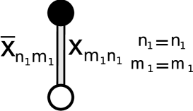
Figure 12. The only possible bipartite Möbius graph with a single black vertex of degree one. In this case the graph is embedded on a copy of the Riemann sphere.

As another example

$$\mathbb{E}({\rm tr}(\mathbf{W}^{2})) =\sum_{m_{1},m_{2}=1}^{M}\sum_{n_{1},n_{2}=1}^{N}\mathbb{E}(X^{*}_{n_{1}m_{1}}X_{m_{1}n_{2}}X^{*}_{n_{2}m_{2}}X_{m_{2}n_{1}})$$

$$=\sum_{m_{1},m_{2}=1}^{M}\sum_{n_{1},n_{2}=1}^{N}\Big{[}\mathbb{E}(X^{*}_{n_{1}m_{1}}X_{m_{1}n_{2}})\mathbb{E}(X^{*}_{n_{2}m_{2}}X_{m_{2}n_{1}})$$

$$\phantom{\sum_{m_{1},m_{2}=1}^{M}\sum_{n_{1},n_{2}=1}^{N}}+\mathbb{E}(X^{*}_{n_{1}m_{1}}X^{*}_{n_{2}m_{2}})\mathbb{E}(\bar{X}_{m_{1}n_{2}}X_{m_{2}n_{1}})$$

$$\phantom{\sum_{m_{1},m_{2}=1}^{M}\sum_{n_{1},n_{2}=1}^{N}}+\mathbb{E}(X^{*}_{n_{1}m_{1}}X_{m_{2}n_{1}})\mathbb{E}(X_{m_{1}n_{2}}X^{*}_{n_{2}m_{2}})\Big{]}$$

$$=16NM^{2}-8NM+16N^{2}M\,,$$

corresponds to the bipartite Möbius graphs in Figure 13.

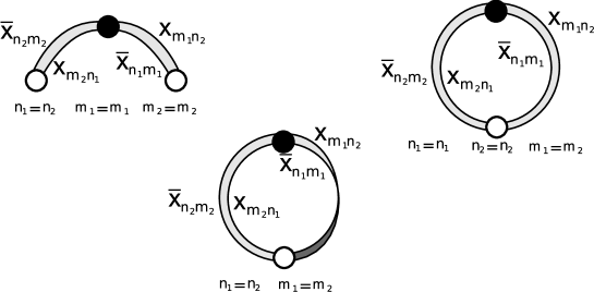
Figure 13. The three possible bipartite Möbius graphs with a single black vertex of degree two. In the top two cases the graph is embedded on a copy of the Riemann sphere, while in the bottom case the graph is embedded on a copy of the projective sphere.

In this case our theorem takes the form.

Theorem 4.2.

With $M=\lambda N$ we find

$$\mathbb{E}({\rm tr}(\mathbf{W}^{j_{1}}){\rm tr}(\mathbf{W}^{j_{2}})\cdots{\rm tr}(\mathbf{W}^{j_{m}}))=N^{n-m}4^{n-m}\sum_{\Gamma}\lambda^{w(\Gamma)}(-2N)^{\chi(\Gamma)}\;,$$

where the sum is over the bipartite Möbius graphs with black vertices having degrees $j_{1},j_{2},\dots,j_{m}$, $n=j_{1}+j_{2}+\dots+j_{m}$ is the number of edges, $w(\Gamma)$ is the number of white vertices, and $\chi(\Gamma)$ is the Euler characteristic.

More generally, suppose that $\mathbf{W}_{1},\mathbf{W}_{2},\dots,\mathbf{W}_{s}$ are $N\times N$ independent quaternionic Wishart with parameters $M_{1},\dots,M_{s}$. Denote $\lambda_{j}=M_{j}/N$. Fix $t:\{1,\dots,n\}\to\{1,\dots,s\}$, and let $\alpha_{1}=1$, $\alpha_{k}=j_{1}+j_{2}+\dots+j_{k-1}+1$, $\beta_{k}=j_{1}+j_{2}+\dots+j_{k}$ denote the ranges under traces. Then

(4.7) $$\frac{1}{(4N)^{n-m}}\mathbb{E}\big{(}\Re({\rm tr}(\mathbf{W}_{t(1)}\dots\mathbf{W}_{t(\beta_{1})}))\Re({\rm tr}(\mathbf{W}_{t(\alpha_{2})}\dots\mathbf{W}_{t(\beta_{2})}))\times\dots{\\ }\dots\times\Re({\rm tr}(\mathbf{W}_{t(\alpha_{m})}\dots\mathbf{W}_{t(\beta_{m})}))\big{)}=\sum_{\Gamma}\lambda_{1}^{w_{1}(\Gamma)}\lambda_{2}^{w_{2}(\Gamma)}\dots\lambda_{s}^{w_{s}(\Gamma)}(-2N)^{\chi(\Gamma)},$$

where the sum is over the bipartite Möbius graphs with $m$ black vertices of degrees $j_{1},\dots,j_{m}$, whose ribbons are colored according to $t$ by one of the colors $1,\dots,s$, and with white vertices that are colored to match the ribbons. Here $w_{j}(\Gamma)$ is the number of white vertices of color $j$, $\chi(\Gamma)$ is the Euler characteristic and $j_{1}+j_{2}+\dots+j_{m}=n$ is the number of edges/ribbons.

Proof.

We begin by expanding out the traces in terms of the matrix entries of $\mathbf{X}$ where $\mathbf{W}=\mathbf{X}^{*}\mathbf{X}$ and $\mathbf{X}$ is an $M\times N$ matrix of quaternionic Gaussian random variables

(4.8) $$\frac{N^{m-n}}{4^{n-m}}\mathbb{E}({\rm tr}(\mathbf{W}^{j_{1}}){\rm tr}(\mathbf{W}^{j_{2}})\cdots{\rm tr}(\mathbf{W}^{j_{m}}))=$$

$$\sum_{\begin{matrix}1\leq a_{1},a_{2},\dots,a_{j_{1}}\leq N\\ 1\leq A_{1},A_{2},\dots,A_{j_{1}}\leq M\\ 1\leq b_{1},b_{2},\dots,b_{j_{2}}\leq N\\ 1\leq B_{1},B_{2},\dots,B_{j_{2}}\leq M\\ \vdots\\ 1\leq C_{1},C_{2},\dots,C_{j_{m}}\leq M\end{matrix}}\begin{matrix}\frac{N^{m-n}}{4^{n-m}}\mathbb{E}(\Re([\mathbf{X}^{*}]_{a_{1}A_{1}}[\mathbf{X}]_{A_{1}a_{2}}[\mathbf{X}^{*}]_{a_{2}A_{2}}[\mathbf{X}]_{A_{2}a_{3}}\dots[\mathbf{X}^{*}]_{a_{j_{1}}A_{j_{1}}}[\mathbf{X}]_{A_{j_{1}}a_{1}})\\ \hfill\Re([\mathbf{X}^{*}]_{b_{1}B_{1}}\dots[\mathbf{X}]_{B_{j_{2}}b_{1}})\dots\Re([\mathbf{X}^{*}]_{c_{1}C_{1}}\dots[\mathbf{X}]_{C_{j_{m}}c_{1}}))\,.\end{matrix}$$

Note that a similar expansion would be found for a multi matrix expression, see below.

From (2.10) it follows that (4.8) can be expanded as a sum over all pairings, and we can assume that the pairs are independent.

We label all such pairings by bipartite Möbius graphs, that is Möbius graphs with labeled black vertices of degree $j_{1},j_{2},\dots,j_{m}$, and unlabeled white vertices of any degree. The half edges of each graph are labeled by $\bar{X}_{A_{1}a_{1}}=\bar{X}_{-1}$, $X_{A_{1}a_{2}}=X_{1}$ and so on. The relations given by this Möbius graph reduce the number of sums over capital indices (which go from 1 to $M$) to $w(\Gamma)$ the number of white vertices, and reduce the number of sums over lower case indices (which go from 1 to $N$) to $f(\Gamma)$ the number of faces of $\Gamma$. Therefore from Theorem 3.2, with $M=\lambda N$, the total contribution from the Wishart Möbius graph $\Gamma$ to the sum is

$$\frac{N^{m-n}}{4^{n-m}}\left[4^{n-m}\lambda^{w(\Gamma)}(-2)^{\chi(\Gamma)}\right]N^{w(\Gamma)+f(\Gamma)}=\lambda^{w(\Gamma)}(-2N)^{\chi(\Gamma)}\,,$$

as $\chi(\Gamma)=m+w(\Gamma)-n+f(\Gamma)$.

The multimatrix version of this proof requires no conceptual changes, but the notation becomes more cumbersome. In this case it is more convenient to index the products by the cycles of a permutation. Put

$$\sigma=(1,\dots,\beta_{1})(\alpha_{2},\dots,\beta_{2})\ldots(\alpha_{m},\dots,n).$$

In this notation, the expansion on the right hand side of (4.8) is replaced by

$$\sum_{a:\{1\dots n\}\to\{1\dots N\}}\mathbb{E}\left(\prod_{c\in\sigma}\Re(\prod_{j\in c}[\mathbf{W}_{t(j)}]_{a(j),a(\sigma(j))})\right)\\ =\sum_{a:\{1\dots n\}\to\{1\dots N\}}\sum_{b\in\mathcal{B}(t)}\mathbb{E}\left(\prod_{c\in\sigma}\Re(\prod_{j\in c}\overline{[{\mathbf{X}}_{t(j)}]}_{b(j)a(j)}[\mathbf{X}_{t(j)}]_{b(j),a(\sigma(j))})\right),$$

where $\mathcal{B}(t)=\{1,\dots,M_{t(1)}\}\times\{1,\dots,M_{t(2)}\}\times\dots\times\{1,\dots,M_{t(n)}\}$.

From (2.10) the expected value can again be expanded as a sum over the pairings, where we can assume that the pairs are independent random variables and the pairings connect only the random variables of the same color $t(j)$. For each bipartite Möbius graph $\Gamma$, the sum over $b\in\mathcal{B}(t)$ contributes a factor of $M_{j}^{w_{j}(\Gamma)}$ per color, where $w_{j}(\Gamma)$ is the number of vertices of color $j$ in $\Gamma$, while the sum over $a$ contributes $N^{f(\Gamma)}$, as in the one-matrix case. Therefore from Theorem 3.2, the left hand side of (4.7) becomes

$$(4N)^{m-n}\sum_{\Gamma}M_{1}^{w_{1}(\Gamma)}\dots M_{s}^{w_{s}(\Gamma)}N^{f(\Gamma)}4^{n-m}(-2)^{\chi(\Gamma)}\\ =N^{m-n}\sum_{\Gamma}N^{w(\Gamma)+f(\Gamma)}(-2)^{\chi(\Gamma)}\prod_{j=1}^{s}\lambda_{j}^{w_{j}(\Gamma)}\\ =\sum_{\Gamma}N^{w(\Gamma)+m+f(\Gamma)-n}(-2)^{\chi(\Gamma)}\prod_{j=1}^{s}\lambda_{j}^{w_{j}(\Gamma)}\\ =\sum_{\Gamma}N^{v(\Gamma)+f(\Gamma)-e(\Gamma)}(-2)^{\chi(\Gamma)}\prod_{j=1}^{s}\lambda_{j}^{w_{j}(\Gamma)}=\sum_{\Gamma}(-2N)^{\chi(\Gamma)}\prod_{j=1}^{s}\lambda_{j}^{w_{j}(\Gamma)}.$$

∎

We remark that the result is again in duality to the formula for real Wishart matrices, where the analogue of (4.7) has the following form:

(4.9) $$\frac{1}{N^{n-m}}\mathbb{E}\big{(}{\rm tr}(\mathbf{W}_{t(1)}\dots\mathbf{W}_{t(\beta_{1})}){\rm tr}(\mathbf{W}_{t(\alpha_{2})}\dots\mathbf{W}_{t(\beta_{2})})\times\dots{\\ }\dots\times{\rm tr}(\mathbf{W}_{t(\alpha_{m})}\dots\mathbf{W}_{t(\beta_{m})})\big{)}=\sum_{\Gamma}\lambda_{1}^{w_{1}(\Gamma)}\lambda_{2}^{w_{2}(\Gamma)}\dots\lambda_{s}^{w_{s}(\Gamma)}N^{\chi(\Gamma)}.$$

For the one-matrix case this can be read out from [10]. For the multivariate case this is a reinterpretation of [2, Theorem 2.10].

The following illustrates a one-matrix version of this duality.

Example 4.2.

Suppose $\mathbf{W}_{\mathbb{R}}$ is $N\times N$ real Wishart matrix with parameter $M$, and let

$$Q_{j_{1},\dots,j_{m}}^{\mathbb{R}}(M,N)=\mathbb{E}({\rm tr}(\mathbf{W}_{\mathbb{R}}^{j_{1}}){\rm tr}(\mathbf{W}_{\mathbb{R}}^{j_{2}})\cdots{\rm tr}(\mathbf{W}_{\mathbb{R}}^{j_{m}})).$$

If $\mathbf{W}_{\mathbb{H}}$ is $N\times N$ quaternion Wishart matrix with parameter $M$, and $n=j_{1}+\dots+j_{m}$, then (4.9) and (4.7) give

$$\mathbb{E}({\rm tr}(\mathbf{W}_{\mathbb{H}}^{j_{1}}){\rm tr}(\mathbf{W}_{\mathbb{H}}^{j_{2}})\cdots{\rm tr}(\mathbf{W}_{\mathbb{H}}^{j_{m}}))=(-2)^{n-m}Q_{j_{1},\dots,j_{m}}^{\mathbb{R}}(-2M,-2N).$$

This is equivalent to [10, Corollary 4.2], as with $\lambda=(j_{1},j_{2},\dots,j_{m})$ in their notation

$$Q_{j_{1},\dots,j_{m}}^{\mathbb{H}}(M,N)=2^{-n}\mathbb{E}({\rm tr}(\mathbf{W}_{\mathbb{H}}^{j_{1}}){\rm tr}(\mathbf{W}_{\mathbb{H}}^{j_{2}})\cdots{\rm tr}(\mathbf{W}_{\mathbb{H}}^{j_{m}}))\\ =(-1)^{n-m}2^{-m}Q_{j_{1},\dots,j_{m}}^{\mathbb{R}}(-2M,-2N);$$

an extra factor of $2^{n}$ in our formula is due to the fact that the quaternion Gaussian law in [10] has the variance of $1/2$ instead of our choice of $1$.

Acknowledgements

The authors thank Gérard Letac for citation [12]. We would like to thank the referee for several substantial corrections.

References

- [1] Bessis, D., Itzykson, C., and Zuber, J. B. Quantum field theory techniques in graphical enumeration. Adv. in Appl. Math. 1, 2 (1980), 109–157.
- [2] Bryc, W. Compound real Wishart and -Wishart matrices. Int. Math. Res. Not. IMRN (2008), Art. ID rnn 079, 42.
- [3] Dumitriu, I., and Edelman, A. Global spectrum fluctuations for the -Hermite and -Laguerre ensembles via matrix models. J. Math. Phys. 47, 6 (2006), 063302, 36.
- [4] Ercolani, N. M., and McLaughlin, K. D. T.-R. Asymptotics of the partition function for random matrices via Riemann-Hilbert techniques and applications to graphical enumeration. Int. Math. Res. Not., 14 (2003), 755–820.
- [5] Goulden, I. P., Harer, J. L., and Jackson, D. M. A geometric parametrization for the virtual Euler characteristics of the moduli spaces of real and complex algebraic curves. Trans. Amer. Math. Soc. 353, 11 (2001), 4405–4427 (electronic).
- [6] Goulden, I. P., and Jackson, D. M. Connection coefficients, matchings, maps and combinatorial conjectures for Jack symmetric functions. Trans. Amer. Math. Soc. 348, 3 (1996), 873–892.
- [7] Goulden, I. P., and Jackson, D. M. Maps in locally orientable surfaces, the double coset algebra, and zonal polynomials. Canad. J. Math. 48, 3 (1996), 569–584.
- [8] Goulden, I. P., and Jackson, D. M. Maps in locally orientable surfaces and integrals over real symmetric matrices. Canad. J. Math. 49, 5 (1997), 865–882.
- [9] Guionnet, A., and Maurel-Segala, E. Combinatorial aspects of matrix models. ALEA Lat. Am. J. Probab. Math. Stat. 1 (2006), 241–279 (electronic).
- [10] Hanlon, P. J., Stanley, R. P., and Stembridge, J. R. Some combinatorial aspects of the spectra of normally distributed random matrices. In Hypergeometric functions on domains of positivity, Jack polynomials, and applications (Tampa, FL, 1991), vol. 138 of Contemp. Math. Amer. Math. Soc., Providence, RI, 1992, pp. 151–174.
- [11] Harer, J., and Zagier, D. The Euler characteristic of the moduli space of curves. Inventiones Mathematicae 85, 3 (1986), 457–485.
- [12] Isserlis, L. On a formula for the product-moment coefficient of any order of a normal frequency distribution in any number of variables. Biometrika 12, 1/2 (1918), 134–139.
- [13] Jackson, D. M. On an integral representation for the genus series for -cell embeddings. Trans. Amer. Math. Soc. 344, 2 (1994), 755–772.
- [14] Janson, S. Gaussian Hilbert spaces, vol. 129 of Cambridge Tracts in Mathematics. Cambridge University Press, Cambridge, 1997.
- [15] Jüngling, K., and Oppermann, R. Effects of spin interactions in disordered electronic systems: loop expansions and exact relations among local gauge invariant models. Z. Phys. B 38, 2 (1980), 93–109.
- [16] Kodama, Y., and Pierce, V. U. Combinatorics of dispersionless integrable systems and universality in random matrix theory, 2008. arxiv:0811.0351.
- [17] Ledoux, M. A recursion formula for the moments of the Gaussian Orthogonal Ensemble. Ann. Inst. H. Poincaré Probab. Statist. (2007). (to appear).
- [18] Leonov, V. P., and Shiryaev, A. N. On a method of semi-invariants. Theor. Probability Appl. 4 (1959), 319–329.
- [19] Maurel-Segala, E. High order expansion of matrix models and enumeration of maps, 2006. arXiv:math.PR/0608192.
- [20] Mkrtchyan, R. The equivalence of and gauge theories. Phys. Letters B105 (1981), 174–176.
- [21] Mulase, Motohico; Waldron, A. Duality of orthogonal and symplectic matrix integrals and quaternionic Feynman graphs. Commun. Math. Phys. 240 (2003), 553–586.
- [22] Speed, T. P. Cumulants and partition lattices. Austral. J. Statist. 25, 2 (1983), 378–388.
- [23] t’Hooft, G. A planar diagram theory for strong interactions. Nuclear Physics B 72 (1974), 461–473.
- [24] Vakhania, N. N. Random vectors with values in quaternion Hilbert space. Theory of Probability and its Applications 43 (1999), 99–115.
- [25] Wegner, F. Algebraic derivation of symmetry relations for disordered electronic systems. Z. Phys. B 49, 4 (1982), 297–302.
- [26] Wick, G. C. The evaluation of the collision matrix. Phys. Rev. 80, 2 (Oct 1950), 268–272.
- [27] Witten, E. Baryons and branes in anti-de Sitter space. J. High Energy Phys., 7 (1998), Paper 6, 39 pp. (electronic).