The long-range interaction

in massless $(\lambda\Phi^{4})_{4}$ theory
P. M. Stevenson

T. W. Bonner Laboratory, Department of Physics and Astronomy,
Rice University, P.O. Box 1892, Houston, TX 77251-1892, USA

Abstract:

Does massless $(\lambda\Phi^{4})_{4}$ theory exhibit spontaneous symmetry breaking (SSB)? The raw 1-loop result implies that it does, but the “RG-improved” result implies the opposite. I argue that the appropriate “low-energy effective theory” is a nonlocal field theory involving an attractive, long-range interaction $\Phi^{2}(x)\Phi^{2}(y)/z^{4}$, where $z=\mid\!x-y\!\mid$. RG improvement then requires running couplings for both this interaction and the original pointlike interaction. A crude calculation in this framework yields SSB even after “RG improvement” and closely agrees with the raw 1-loop result.

1 Introduction

Although seemingly the simplest renormalizable quantum field theory, the 4-dimensional $\lambda\Phi^{4}$ theory differs from other paradigm theories, QED and QCD – and, as yet, there is no experimental confirmation that we understand the theory correctly. The issue is important because of the relevance of $\lambda\Phi^{4}$ theory to the Higgs mechanism and to inflationary cosmology.

One basic issue is the nature of the phase transition as one varies the renormalized-mass $m$: Is it a second-order transition occurring at $m^{2}=0$, or is it a first-order transition occurring at some small but positive value of $m^{2}$? Equivalently, one can ask if the massless theory is still in the symmetric phase or not. The dilemma goes back to Coleman and Weinberg [1] who found that in massless $\lambda\Phi^{4}$ the 1-loop effective potential (1LEP) predicts spontaneous symmetry breaking (SSB), but that “renormalization-group improvement” (RGI) contradicts that result. (By contrast, in Scalar Electrodynamics they found that RGI confirmed the 1-loop prediction of SSB.) It is the contradiction between 1LEP and RGI in $\lambda\Phi^{4}$ theory that is the main concern of this paper.

2 A particle-language argument

A very physical argument for a first-order transition was given in Ref. [2]. Consider the $\lambda\Phi^{4}$ theory with a small, positive renormalized mass $m$ and focus on the particles (“phions”) and their interactions. The fundamental interaction is the pointlike repulsive interaction (Fig. 1(a)). However, the ‘fish’ diagram (Fig. 1(b)) induces a long-range attractive interaction, proportional to $-1/r^{3}$ if we ignore the phion mass [3, 2]. Consider a large number $\mathsf{N}$ of phions contained in a large box of volume $\mathsf{V}$ with periodic boundary conditions. What is the lowest energy of this system? Naturally, to minimize the kinetic energy we would put almost all the phions into the $\mathbf{k}=0$ mode. Thus, if there were no interactions, the energy would just be the sum of the rest-energies, $\mathsf{N}m$. Two-body interactions add a term given by the number of pairs (${\scriptstyle{\frac{1}{2}}}\mathsf{N}(\mathsf{N}-1)\approx{\scriptstyle{\frac{1}{2}}}\mathsf{N}^{2}$) multiplied by the average interparticle potential energy $\bar{u}$, giving a total energy

$$E_{\mathrm{tot}}=\mathsf{N}m+{\scriptstyle{\frac{1}{2}}}\mathsf{N}^{2}\bar{u}.$$ (1)

Effects from three-body or multi-body interactions will be negligible provided that the phion gas is dilute.

Figure 1: (a) The fundamental interaction.  (b) The “fish” diagram, which induces a long-range interaction.

If the interparticle potential is $U(r)$ and we assume that the particles are uniformly distributed over the box, which is true if almost all the particles are in the $\mathbf{k}=0$ mode, then

$$\bar{u}\sim{\frac{{1}}{{\mathsf{V}}}}\int\!d^{3}r\,U(r).$$ (2)

Hence, we obtain an energy density

$$\mathcal{E}\equiv E_{\mathrm{tot}}/\mathsf{V}=nm+{\scriptstyle{\frac{1}{2}}}n^{2}\int\!d^{3}r\,U(r),$$ (3)

where $n\equiv\mathsf{N}/\mathsf{V}$. The interparticle potential $U(r)$ consists of the pointlike repulsion term plus the $-1/r^{3}$ term. The former integrates to some constant, but the latter requires cutoffs at both small and large $r$, giving

$$\mathcal{E}=nm+C_{1}n^{2}-C_{2}n^{2}\ln(r_{\mathrm{max}}/r_{0}),$$ (4)

where $C_{1},C_{2}$ are some positive constants. The ultraviolet divergence is not unexpected and $1/r_{0}$ is naturally identified with the ultraviolet cutoff needed in the field theory. The infrared divergence arises, of course, from neglecting the mass of the exchanged phions in the ‘fish’ diagram; actually the $-1/r^{3}$ potential is exponentially suppressed at distances $r>1/(2m)$. However, when $m$ is very small another consideration is more important; namely, that the long-distance attraction between two phions will be “screened” by other phions that interpose themselves. This consideration implies an effective $r_{\mathrm{max}}$ that depends on the density $n$.

[The virtual phions being exchanged undergo multiple scatterings with the background $\mathbf{{k}=0}$ phions (See Fig. 2). Each collision corresponds to a mass insertion and the resulting geometric series changes the mass to $M^{2}=m^{2}+\lambda n/m$. The mass $M$ represents the mass of a quasiparticle excitation of the phion condensate; i.e., it is the Higgs boson mass. In the small-$m$ regime of interest $M\approx\lambda n/m$ and so $r_{\mathrm{max}}=1/(2M)\propto 1/\sqrt{n}$.]

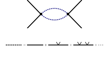
Figure 2: Screening of the long-range interaction due to multiple collisions with background phions.

Hence, $\mathcal{E}$ is given by a sum of $n$, $n^{2}$ and $n^{2}\ln n$ terms which represent, respectively, the rest-energy cost, the repulsion energy cost, and the energy gain from the long-range attraction. If the rest-mass $m$ is small enough, then the $n^{2}\ln n$ term’s negative contribution will result in an energy density whose global minimum is not at $n=0$ but at some specific, non-zero density $n_{v}$. That is, even though the ‘empty’ state is locally stable, it can decay by spontaneously generating particles so as to fill the box with a dilute condensate of density $n_{v}$. This condensate is the the SSB vacuum. In field-theory terms the particle density $n$ is proportional to the classical field squared, $n={\scriptstyle{\frac{1}{2}}}m\phi^{2}$, and the energy density as a function of $n$ is the field-theoretic effective potential: $\mathcal{E}(n)\equiv V_{\mathrm{eff}}(\phi)$. This argument, then, reproduces the form of the 1LEP, with $\phi^{2}$, $\phi^{4}$, and $\phi^{4}\ln\phi^{2}$ terms.

3 Implications for RG improvement

An important moral of the above argument is that in nearly-massless $\lambda\Phi^{4}$ theory there are really two interactions; a short-range repulsion and a long-range attraction, the latter induced by the former. Successful use of RG methods requires that we first identify all appropriate interactions (“relevant” and “marginal”) and then consider how the strengths of those interactions change with scale. The suggestion here is that we need to consider two running couplings.

The usual RGI procedure in massless $\lambda\Phi^{4}$ theory considers only the pointlike $\lambda\phi^{4}$ interaction. The main effect of loop diagrams, it asserts, is just to renormalize $\lambda$, resulting in a running coupling $\lambda_{R}(\mu)$ that runs with renormalization scale $\mu$. The effective potential, to lowest order, is then the classical potential with $\lambda$ replaced by $\lambda_{R}(\phi)$:

$$V_{\mathrm{eff}}^{\mathrm{RGI}}=\frac{\lambda_{R}(\phi)}{4!}\phi^{4}.$$ (5)

Since, to leading order, $\lambda_{R}(\phi)$ is proportional to $1/\ln\phi^{2}$, this RGI effective potential does not show SSB. Higher-order versions of this RGI procedure do not change this qualitative result.

However, when we contemplate the “fish” diagram (Fig. 1(b)), we see that, while its short-distance part containing the ultraviolet divergence does indeed contribute to renormalizing $\lambda$, its long-distance part is actually creating a physically distinct interaction, the long-range attraction (a $-1/r^{3}$ interparticle potential in the particle language of the previous section). If we now switch to a manifestly covariant, Euclideanized functional-integral formalism, the “fish” diagram will generate a term in the effective action proportional to

$$\int\!d^{4}x\int\!d^{4}y\,\Phi^{2}(x)(\mathcal{G}_{xy})^{2}\Phi^{2}(y),$$ (6)

where $\mathcal{G}_{xy}$ is the $x$-space propagator, proportional to $1/\!\mid\!x-y\!\mid^{2}$ if we neglect the phion mass. This term is inherently non-local. While a fundamental Lagrangian must be local, for reasons of causality, an effective Lagrangian can, and in general does, contain non-local terms. In theories without infrared sensitivity one may make a derivative expansion of the non-local terms as a series of local terms, but that option is not possible here.

This paper does not attempt to present a comprehensive formalism embodying these ideas. Instead, for maximal simplicity, we set aside some important issues (precisely how the non-local term is generated and how to avoid double counting) and simply start directly with a non-local action.

4 The nonlocal model

Consider then a nonlocal effective theory described by the following Euclidean action:

$$S=\int\!d^{4}\,x\,\frac{1}{2}\partial_{\mu}\Phi\,\partial^{\mu}\Phi+\int\!d^{4}x\!\int\!d^{4}y\,\,\Phi^{2}(x)U(x-y)\Phi^{2}(y),$$ (7)

where the interaction kernel $U(z)$ is a function only of the Euclidean distance $z=\sqrt{z_{\mu}z^{\mu}}$. It consists of a short-range repulsive core and a long-range attractive tail:

$$U=U_{\mathrm{core}}+U_{\mathrm{tail}},$$ (8)

where

$$U_{\mathrm{core}}(z)=\frac{\lambda}{4!}f(z;z_{0})\quad\quad\quad{\scriptstyle{(0<z<z_{0})}},$$ (9)

and

$$U_{\mathrm{tail}}(z)=-\frac{\zeta}{z^{4}}\quad\quad\quad{\scriptstyle{(z_{0}<z<z_{\mathrm{max}})}}.$$ (10)

Here, $\lambda$ and $\zeta$ are positive parameters and $\int_{0}^{z_{0}}d^{4}zf(z;z_{0})\equiv 1$ so that $f(z;z_{0})$ approaches $\delta^{(4)}(z)$ as $z_{0}\to 0$. It is convenient to define a positive, dimensionless coupling $\eta$ for the long-range interaction by:

$$\frac{\eta}{4!}\equiv-\int\!d^{4}z\,U_{\mathrm{tail}}(z)=2\pi^{2}\zeta\ln\left(\frac{z_{\mathrm{max}}}{z_{0}}\right),$$ (11)

so that

$$\lambda_{\mathrm{tot}}\equiv\lambda-\eta$$ (12)

represents the “total” interaction strength, in the sense that

$$\frac{\lambda_{\mathrm{tot}}}{4!}=\int d^{4}z\left(U_{\mathrm{core}}(z)+U_{\mathrm{tail}}(z)\right).$$ (13)

The theory is also to be regulated by an ultraviolet cutoff $\Lambda$ by excluding all momentum modes with $p>\Lambda$. Note that, at this stage, $\Lambda,z_{0},z_{\mathrm{max}}$ and $\lambda,\eta$ are all independent, free parameters of the model theory. Later on we shall be interested in taking limits where $\Lambda\to\infty$, $z_{0}\to 0$, and $z_{\mathrm{max}}\to\infty$. (Note that $z_{\mathrm{max}}$ can be thought of as $1/(2m)$, where $m$ is the phion mass, which is otherwise neglected.)

The aim now is to compute the effective potential of this model theory to second order in a double perturbation expansion in powers of the renormalized $\lambda$ and $\eta$ couplings. This second-order result can be obtained from the 1-loop calculation. To begin, one re-writes the action (7) after shifting the field, $\Phi(x)=\phi+h(x)$:

$$S=\mathcal{V}\,\frac{\lambda_{\mathrm{tot}}}{4!}\phi^{4}+\frac{1}{2}\int\!d^{4}x\!\int\!d^{4}y\,h(x)\mathcal{G}^{-1}_{xy}h(y)+(h^{3},h^{4}{\mbox{\rm terms}}),$$ (14)

where $\mathcal{V}$ is the infinite spacetime volume factor $\int\!d^{4}x$, and the inverse propagator is

$$\mathcal{G}^{-1}_{xy}=\left(-\partial^{2}+{\scriptstyle{\frac{1}{6}}}\lambda_{\mathrm{tot}}\phi^{2}\right)\delta^{(4)}(x-y)+8\phi^{2}U(x-y).$$ (15)

Fourier transforming to momentum space leads to

$$\tilde{\mathcal{G}}^{-1}(p)=p^{2}+{\scriptstyle{\frac{1}{6}}}\lambda_{\mathrm{tot}}\phi^{2}+g_{c}(p)+g_{t}(p),$$ (16)

with

$$g_{c}(p)=8\phi^{2}\int\!d^{4}z\,e^{ip.z}\,U_{\mathrm{core}}(z)\quad\quad(\to{\scriptstyle{\frac{1}{3}}}\lambda\phi^{2}\quad{\mbox{\rm for}}\quad z_{0}\to 0),$$ (17)

$$g_{t}(p)=8\phi^{2}\int\!d^{4}z\,e^{ip.z}\,U_{\mathrm{tail}}(z)=-{\scriptstyle{\frac{1}{3}}}\eta\phi^{2}\left(1-\frac{(S(pz_{\mathrm{max}})-S(pz_{0}))}{\ln(z_{\mathrm{max}}/z_{0})}\right),$$ (18)

where

$$S(u)=-2\int_{0}^{u}\frac{dv}{v^{2}}(J_{1}(v)-{\scriptstyle{\frac{1}{2}}}v)$$ (19)

and $J_{1}(v)$ is a Bessel function. $S(u)$ can be expressed in terms of a hypergeometric function;

$$S(u)=\frac{1}{16}u^{2}F_{2,2,3}^{1,1}(-{\scriptstyle{\frac{1}{4}}}u^{2})$$ (20)

and its small- and large-argument behaviours are

$$S(u)\sim\frac{1}{16}u^{2}\quad\quad\quad(u\to 0),$$ (21)

$$S(u)\sim\ln(u/\sigma)-{\scriptstyle{\frac{1}{2}}}\quad\quad(u\to\infty),$$ (22)

with $\sigma=2e^{-\gamma}=1.12\ldots$, where $\gamma$ is the Euler constant. (In fact, the above equations provide a good qualitative description of $S(u)$ for $u\lesssim 2.8$ and $u\gtrsim 2.8$, respectively.) Note that $g_{t}(p)$ is $-{\scriptstyle{\frac{1}{3}}}\eta\phi^{2}$ at $p=0$ and tends to zero as $p\to\infty$.

5 1LEP for the nonlocal model

A full calculation of the 1-loop effective potential in this nonlocal model, valid for a wide range of the parameters $\Lambda,z_{0},z_{\mathrm{max}}$, has been carried out in collaboration with S. A. Hassan [4]. Here, for maximal simplicity, we consider a limit in which $z_{\mathrm{max}}\rightarrow\infty$ (i.e., $m\rightarrow 0$) before taking the $\Lambda\rightarrow\infty$ and $z_{0}\rightarrow 0$ limits. (The full calculation reproduces our results below provided $\mid\!\ln(mz_{0})\!\mid\gg\mid\!\ln(M_{v}z_{0})\!\mid$.)  Then, for all momenta in the range $1/z_{\mathrm{max}}\ll p\ll 1/z_{0}$ (which will become essentially all finite, non-zero momenta) the function $g_{t}(p)$ becomes negligible, of order $\eta\phi^{2}/\ln(z_{\mathrm{max}}/z_{0})$. However, for $p=0$, we have, as always, $g_{t}(p=0)=-{\scriptstyle{\frac{1}{3}}}\eta\phi^{2}$. Thus, the bare propagator has a discontinuity at zero momentum:

$$\tilde{\mathcal{G}}(p)=\left\{\begin{array}[c]{ll}{\scriptstyle{\frac{1}{2}}}\lambda_{\mathrm{tot}}\phi^{2}&\quad\quad p=0\\ p^{2}+M^{2}&\quad\quad p\neq 0\end{array}\right.$$ (23)

with

$$M^{2}\equiv M^{2}(\phi)=\left({\scriptstyle{\frac{1}{6}}}\lambda_{\mathrm{tot}}+{\scriptstyle{\frac{1}{3}}}\lambda\right)\phi^{2}={\scriptstyle{\frac{1}{2}}}(\lambda-{\scriptstyle{\frac{1}{3}}}\eta)\phi^{2}.$$ (24)

In this limit the 1-loop effective potential can then be obtained immediately as

$$V_{\mathrm{eff}}^{\mathrm{1-loop}}(\phi)=\frac{\lambda_{\mathrm{tot}}}{4!}\phi^{4}+\frac{1}{2}\int\!\frac{d^{4}p}{(2\pi)^{4}}\ln(p^{2}+M^{2}).$$ (25)

After subtracting an infinite constant and removing all $\phi^{2}$ terms, corresponding to a mass renormalization condition $\left.d^{2}V_{\mathrm{eff}}/d\phi^{2}\right|_{\phi=0}=0$, this becomes

$$V_{\mathrm{eff}}^{\mathrm{1-loop}}(\phi)=\frac{\phi^{4}}{4!}\left((\lambda-\eta)-\frac{3}{16\pi^{2}}(\lambda-{\scriptstyle{\frac{1}{3}}}\eta)^{2}\left(\ln\frac{\Lambda}{M}+\frac{1}{4}\right)\right).$$ (26)

Obviously, this expression reduces to the usual one when $\eta=0$, but note that now the first term involves $\lambda-\eta$ while the second involves a different combination $\lambda-{\scriptstyle{\frac{1}{3}}}\eta$. One may now proceed to renormalize perturbatively by defining renormalized couplings $\lambda_{R},\eta_{R}$ to absorb the ultraviolet divergence. At first sight, it seems that one can only determine the divergence present in the combination $\lambda-\eta$. However, two simple arguments lead to a unique solution: (i) the short-range interaction, $\lambda$, should only be renormalized by short-range interactions — since a short-range interaction modified by a long-range interaction would cease to be short range; (ii) Although the short-range interaction, acting twice, induces a long-range interaction, there is no $\ln\Lambda$ divergence involved in the calculation. Argument (i) implies that $\lambda_{R}$ involves only $\lambda$, while argument (ii) implies that $\eta_{R}$ involves $\ln\Lambda$ divergences only in the $\eta\lambda$ and $\eta^{2}$ terms, not in the $\lambda^{2}$ term. Thus, the renormalization is accomplished by

$$\lambda_{R}(\mu)=\lambda-\lambda^{2}\left(\frac{3}{16\pi^{2}}\right)\left(\ln\frac{\Lambda}{\mu}+a_{1}\right)+\ldots,$$ (27)

$$\eta_{R}(\mu)=\eta+\eta^{2}\left(\frac{1}{48\pi^{2}}\right)\left(\ln\frac{\Lambda}{\mu}+a_{2}\right)+\eta\lambda\left(-\frac{1}{8\pi^{2}}\right)\left(\ln\frac{\Lambda}{\mu}+a_{3}\right)+a_{4}\lambda^{2}+\ldots,$$ (28)

where $\mu$ is some arbitrary renormalization scale and $a_{1},a_{2},a_{3}$ are arbitrary, renormalization-scheme-dependent finite constants. The $a_{4}$ term is a “calculable coefficient”:

$$a_{4}=\frac{3}{2\pi^{2}}\lambda^{2}\ln(z_{\mathrm{max}}/z_{0})$$ (29)

except that it involves an infinite $\ln(z_{\mathrm{max}}/z_{0})$ factor from converting $\zeta$ to $\eta$ (see Eq. (11)). However, all that matters here is that $a_{4}$ has no $\Lambda$ or $\mu$ dependence and so will not affect any beta functions. In fact, one may argue that this term should simply be subtracted to avoid double counting of the long-range interaction.

[Eqs. (27), (28) can also be deduced from the 1-loop diagrams for the 4-point function in this nonlocal theory. The correct combinatorial factors, reported in Fig. 3, can be found from a straightforward, if tedious, calculation of the fourth functional derivative of the generating functional $Z[j]$ associated with the nonlocal action (7).]

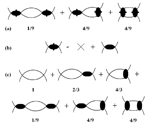
Figure 3: (a) With a nonlocal interaction $U$ the fish diagram generalizes to three distinct diagrams with combinatoric weights as shown. Substituting $U=U_{\mathrm{core}}+U_{\mathrm{tail}}$, as shown in (b), leads to the weights shown in (c). The second and fourth diagrams in (c) produce the $-\eta\lambda$ and $\eta^{2}$ divergences in Eq. (28).

Substituting for the bare parameters (using the inverse of Eqs. (27), (28)) and re-expanding in powers of the renormalized couplings, dropping terms cubic or higher, leads to the renormalized perturbative result. It consists solely of $\phi^{4}$ and $\phi^{4}\ln\phi$ terms, so that if we define $v$ as the location of the minimum (i.e., the vacuum expectation of $\phi$) we may write the result as

$$V_{\mathrm{eff}}^{\mathrm{pert}}=\frac{M_{R}^{4}}{64\pi^{2}}\left(\ln\frac{\phi^{2}}{v^{2}}-\frac{1}{2}\right),$$ (30)

with

$$M_{R}^{2}=\frac{1}{2}\left(\lambda_{R}-{\scriptstyle{\frac{1}{3}}}\eta_{R}\right)\phi^{2}.$$ (31)

(Note that the constants $a_{1},\ldots,a_{4}$ do not appear in this result; they are subsumed in $v$.)

Thus, in the non-local model, just as in the usual massless $(\lambda\Phi^{4})_{4}$ theory, the one-loop result shows SSB. The question, though, is whether or not this result persists after “RG improvement.”

6 “Improved” RG improvement

We next consider the RG-improvement procedure in the nonlocal model. The RG beta functions follow immediately from Eqs. (27), (28) above:

$$\beta_{\lambda}(\lambda_{R})\equiv\mu\frac{\partial\lambda_{R}}{\partial\mu}=\frac{3}{16\pi^{2}}\lambda_{R}^{2}+\ldots,$$ (32)

$$\beta_{\eta}(\eta_{R},\lambda_{R})\equiv\mu\frac{\partial\eta_{R}}{\partial\mu}=-\frac{1}{48\pi^{2}}\eta_{R}^{2}+\frac{1}{8\pi^{2}}\eta_{R}\lambda_{R}+\ldots.$$ (33)

Integrating (32) to leading order gives, as usual,

$$\lambda_{R}(\mu)=\frac{16\pi^{2}}{3}\frac{1}{\ln\mu_{0}/\mu},$$ (34)

where $\mu_{0}$ is the Landau-pole scale. Substituting into (33) yields the differential equation

$$\mu\frac{\partial\eta_{R}}{\partial\mu}-\frac{2}{3}\frac{\eta_{R}}{\ln\mu_{0}/\mu}=-\frac{1}{48\pi^{2}}\eta_{R}^{2}.$$ (35)

Multiplying by the integrating factor $(\ln\mu_{0}/\mu)^{2/3}$, the left-hand side becomes a total derivative, yielding the solution

$$\eta_{R}(\mu)=\frac{16\pi^{2}}{u^{2}(u_{c}-u)},$$ (36)

where

$$u\equiv(\ln\mu_{0}/\mu)^{1/3}$$ (37)

and $u_{c}$ is a constant of integration. The $\eta_{R}$ coupling thus has singularities at both the Landau scale $\mu_{0}$ ($u=0$) and at a scale $\mu_{c}$ ($u=u_{c}$). To have $\eta_{R}$ positive and a region where both $\lambda_{R}$ and $\eta_{R}$ are small requires $\mu_{c}\ll\mu_{0}$. That means that $u_{c}\equiv(\ln\mu_{0}/\mu_{c})^{1/3}$ should be a large number. Figure 4 shows the running couplings as a function of $u$.

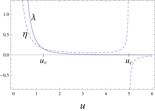
Figure 4: Running couplings (divided by $16\pi^{2}$) as functions of $u\equiv(\ln(\mu_{0}/\mu))^{1/3}$. (Shown for $u_{c}=5$.)

The “RG improved” effective potential, to leading order, is obtained by taking the classical potential (the first term of Eq. (14) with $\mathcal{V}$ divided out) and replacing the bare coupling with a running coupling: i.e.,

$$V_{\mathrm{eff}}^{\mathrm{RGI}}(\phi)=\frac{\lambda_{\mathrm{tot}}^{R}(\phi)}{4!}\phi^{4},$$ (38)

where

$$\lambda_{\mathrm{tot}}^{R}(\mu)=\lambda_{R}(\mu)-\eta_{R}(\mu)=\frac{16\pi^{2}}{3}\frac{(u_{c}-4u)}{u^{3}(u_{c}-u)},$$ (39)

and the renormalization scale $\mu$ is chosen to be $\phi$. Taking the derivative of $V_{\mathrm{eff}}^{\mathrm{RGI}}(\phi)$ (noting that $\mu du/d\mu=-1/(3u^{2})$) yields

$$\frac{dV_{\mathrm{eff}}^{\mathrm{RGI}}}{d\phi}=\frac{2\pi^{2}}{9}\phi^{3}\frac{\left[4u^{3}(4u-u_{c})(u-u_{c})+(2u-u_{c})^{2}\right]}{u^{6}(u_{c}-u)^{2}}.$$ (40)

One sees that the factor in square brackets has a non-trivial root close to $u={\scriptstyle{\frac{1}{4}}}u_{c}$:

$$u_{v}=\frac{1}{4}u_{c}\left(1+\frac{16}{3}\frac{1}{u_{c}}^{3}+\mathcal{O}\left(\frac{1}{u_{c}^{6}}\right)\right).$$ (41)

This means that $V_{\mathrm{eff}}^{\mathrm{RGI}}(\phi)$ has an SSB minimum at $\phi=v$, where $(\ln\mu_{0}/v)^{1/3}=u_{v}$, that is $v=\mu_{0}\exp(-u_{v}^{3})$. The form of $V_{\mathrm{eff}}^{\mathrm{RGI}}(\phi)$ is shown in Fig. 5. For large $u_{c}$ the RGI effective potential is very close to the “unimproved” perturbative result of Eq. (30), except for a weak pole at very small $\phi$, corresponding to the infrared pole in $\eta_{R}$ at $u=u_{c}$. It seems reasonable to dismiss this infrared pole as an artifact of the leading-order approximation, perhaps signalling some complex physics in the far infrared. Higher terms in the $\eta$ beta function might well remove the pole, giving a “freezing” of $\eta$ in the infrared.

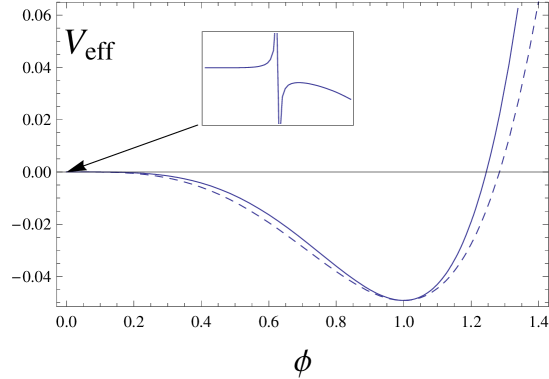
Figure 5: RGI effective potential (solid line) compared with the raw perturbative result (dashed curve). Units such that $v=1$. The RGI result has a weak pole at a tiny value of $\phi$. In this example $u_{c}=5$. For larger $u_{c}$ the two curves become almost indistinguishable and the pole, here at $\phi\approx 4\times 10^{-54}$, retreats to exponentially smaller values of $\phi$.

The important point is that one now has essential agreement between the perturbative and RGI results, provided $u_{c}$ is large (which is necessary for the renormalized couplings to be small at the scale $v$). In the conventional treatment the RGI effective potential cannot show SSB because the running coupling $\lambda_{R}(\phi)$ must remain positive. Here, although $\lambda_{R}$ remains positive, the RGI effective potential is governed by $\lambda_{\mathrm{tot}}^{R}=\lambda_{R}-\eta_{R}$ which can and does go negative. The SSB vacuum is very close to $u={\scriptstyle{\frac{1}{4}}}u_{c}$ where $\lambda_{R}$ and $\eta_{R}$ cancel. Hence, the inverse propagator (23) nearly vanishes at $p=0$, in accord with [5].

7 Conclusions

The massless $(\lambda\Phi^{4})_{4}$ theory has two physically distinct interactions – the fundamental short-range repulsion and the induced long-range attraction. Conventional RGI ignores the latter. RGI including both interactions leads to SSB and closely agrees with the raw 1-loop result.

Acknowledgments: Discussions with S. A. Hassan and M. Consoli are gratefully acknowledged.

References

- [1] S. Coleman and E. Weinberg, Phys. Rev. D7, 1888 (1973).
- [2] M. Consoli and P. M. Stevenson, Intl. J. of Mod. Phys. A15, 133 (2000).
- [3] G. Feinberg and J. Sucher, Phys. Rev. 166, 1683 (1968); G. Feinberg, J. Sucher, and C. K. Au, Phys. Rep. 180, 85 (1989).
- [4] S. Asif Hassan, M.S. Thesis, Rice University, 2006 (unpublished).
- [5] M. Consoli, Phys. Rev. D 65, 105017 (2002).