Abstract

We study loop operators of $5d$ $\mathcal{N}=1$ SYM in $\Omega$ background. For the case of $U(1)$ theory, the generating function of correlation functions of the loop operators reproduces the partition function of melting crystal model with external potential. We argue the common integrable structure of $5d$ $\mathcal{N}=1$ SYM and melting crystal model.

1 Introduction

It is shown in [1] that the Seiberg-Witten solutions [2] of $4d$ $\mathcal{N}=2$ supersymmetric gauge theories emerge through random partition, where Nekrasov’s formulas [1, 3] for these gauge theories are understood as the partition functions of random partition. The integrable structure of random partition is elucidated in [4], and thereby the integrability of correlation functions among single-traced chiral observables is explained. Such an extension of the Seiberg-Witten geometries also becomes attractive to understand $4d$ $\mathcal{N}=1$ supersymmetric gauge theories by providing a powerful tool [5].

Integrable structure of melting crystal model with external potential is clarified in [6]. Melting crystal model, known as random plane partition has a significant relation with $5d$ $\mathcal{N}=1$ supersymmetric gauge theories. Nekrasov’s formula for these gauge theories can be retrieved from the partition function of melting crystal model [7], where the model is interpreted as a $q$-deformed random partition. It is argued [6] a relation between loop operators of $5d$ $\mathcal{N}=1$ supersymmetric Yang-Mills (SYM) and external potentials of the melting crystal model.

We start Section 2 with providing a brief review about $5d$ $\mathcal{N}=1$ SYM in $\Omega$ background [8]. We introduce loop operators of this theory. Computation of correlation functions among these operators is discussed. Generating function of the correlation functions of $U(1)$ theory reproduces the partition function of the aforementioned melting crystal model. In Section 3 we discuss a common integrable structure of $5d$ $\mathcal{N}=1$ SYM in $\Omega$ background and melting crystal model for the case of the $U(1)$ theory. In Section 4 we present an extension of the Seiberg-Witten geometry of the $U(1)$ theory by using the loop operators.

2 Loop operators of $5d$ $\mathcal{N}=1$ SYM in $\Omega$ background

We first consider an ordinary $5d$ $\mathcal{N}=1$ SYM on $\mathbb{R}^{4}\times S^{1}$. Let $E$ be the $SU(N)$-bundle on $\mathbb{R}^{4}$ with $c_{2}(E)=n\geq 0$. A gauge bundle of this theory is the $SU(N)$-bundle $\pi^{*}E$ on $\mathbb{R}^{4}\times S^{1}$ pulled back from $\mathbb{R}^{4}$. $\pi$ is the projection from $\mathbb{R}^{4}\times S^{1}$ to $\mathbb{R}^{4}$. All the fields in the vector multiplet are set to be periodic along $S^{1}$. The bosonic ingredients are a $5d$ gauge potential $A_{M}(x,t)dx^{M}$ and a scalar field $\varphi(x,t)$ taking the value in $su(N)$. These describe a $5d$ Yang-Mills-Higgs system. The gauge potential can be separated into two parts $A_{\mu}(x,t)dx^{\mu}$ and $A_{t}(x,t)dt$, respectively the components of the $\mathbb{R}^{4}$- and the $S^{1}$-directions. Let $\mathcal{A}_{E}$ be the infinite dimensional affine space consisting of all the gauge potentials on $E$. $A_{\mu}(x,t)dx^{\mu}$ describes a loop $A(t)$ in $\mathcal{A}_{E}$, where the loop is parametrized by the fifth-dimensional circle. As for $A_{t}(x,t)$, together with $\varphi(x,t)$, the combination $A_{t}+i\varphi$ describes a loop $\phi(t)$ in $\Omega^{0}(\mathbb{R}^{4},\mbox{ad}E\otimes\mathbb{C})$, the space of all the sections of $\mbox{ad}E\otimes\mathbb{C}$, where ad$E$ is the adjoint bundle on $\mathbb{R}^{4}$ with fibre $su(N)$. Taking account of the periodicity, the same argument is also applicable to the gauginos. The vector multiplet thereby describes a loop in the configuration space of the $4d$ theory. In the case of the Yang-Mills-Higgs system, the loop $A(t)$ gives a family of covariant differentials on $E$ as $d_{A(t)}=d+A(t)$. For the loop $\phi(t)$, since it involves $A_{t}(x,t)$, it becomes convenient to introduce the differential operator

$$\mathcal{H}(t)\equiv\frac{d}{dt}+\phi(t)\,.$$ (2.1)

2.1 $5d$ $\mathcal{N}=1$ SYM in $\Omega$ background

Via the standard dimensional reductions, $6d$ $\mathcal{N}=1$ SYM gives lower dimensional Yang-Mills theories with $8$ supercharges, including the above theory. Furthermore, the dimensional reductions in the $\Omega$ background provide powerful tools to understand these theories [8]. The $\Omega$ background is a $6d$ gravitational background on $\mathbb{R}^{4}\times T^{2}$ described by a metric of the form: $ds^{2}=\sum_{\mu=1}^{4}(dx^{\mu}-\sum_{a=5,6}V_{a}^{\mu}dx^{a})^{2}+\sum_{a=5,6}(dx^{a})^{2}\,,$ where two vectors $V_{5}^{\mu},V_{6}^{\mu}$ generate rotations on two-planes $(x^{1},x^{2})$ and $(x^{3},x^{4})$ in $\mathbb{R}^{4}$. By letting $V_{1}=x^{2}\frac{\partial}{\partial x^{1}}-x^{1}\frac{\partial}{\partial x^{2}}$ and $V_{2}=x^{4}\frac{\partial}{\partial x^{3}}-x^{3}\frac{\partial}{\partial x^{4}}$, they are respectively the real part and the imaginary part of the combination

$$V_{\epsilon_{1},\epsilon_{2}} \equiv \epsilon_{1}V_{1}+\epsilon_{2}V_{2}\,,\hskip 17.07164pt\epsilon_{1},\epsilon_{2}\in\mathbb{C}.$$ (2.2)

The above combination is expressed in component as $V_{\epsilon_{1},\epsilon_{2}}=\Omega^{\mu}_{~{}\nu}x^{\nu}\frac{\partial}{\partial x^{\mu}}$.

To see the dimensional reduction in the $\Omega$-background, we first consider the bosonic part of the $5d$ SYM. The corresponding Yang-Mills-Higgs system is modified from the previous one. However, the system is eventually controlled by replacing $\mathcal{H}(t)$ with

$$\mathcal{H}_{\epsilon_{1},\epsilon_{2}}(t)\equiv\mathcal{H}(t)+\mathcal{K}_{\epsilon_{1},\epsilon_{2}}(t)\,.$$ (2.3)

Here $\mathcal{K}_{\epsilon_{1},\epsilon_{2}}(t)$ is an another differential operator of the form [9]

$$\mathcal{K}_{\epsilon_{1},\epsilon_{2}}(t)\equiv V_{\epsilon_{1},\epsilon_{2}}^{\mu}\partial_{A(t)\,\mu}+\frac{1}{2}\Omega^{\mu\nu}\mathcal{J}_{\mu\nu}\,,$$ (2.4)

where $\mathcal{J}_{\mu\nu}$ denote the $SO(4)$ Lorentz generators of the system. This operator generates a $T^{2}$-action by taking the commutators with $d_{A(t)}$ and $\mathcal{H}(t)$. For instance, we have

$$[d_{A(t)},\mathcal{K}_{\epsilon_{1},\epsilon_{2}}(t)]=-\iota_{V_{\epsilon_{1},\epsilon_{2}}}F_{A(t)}\,.$$ (2.5)

The right hand side is precisely the transformation brought about on $\mathcal{A}_{E}$ by the infinitesimal rotation $\delta x^{\mu}=-V^{\mu}_{\epsilon_{1},\epsilon_{2}}$.

The supercharges $Q_{\alpha a}$ and $\bar{Q}^{\dot{\alpha}}_{a}$ are realized in a way different from the case of $\epsilon_{1}=\epsilon_{2}=0$. Note that we use the $4d$ notation such that $\alpha,\dot{\alpha}$ and $a$ denote the indices of the Lorentz group $SU(2)_{L}\times SU(2)_{R}$ and the R-symmetry $SU(2)_{I}$. By the standard argument, we may interpret the $5d$ SYM as a topological field theory. Actually, by regarding the diagonal $SU(2)$ of $SU(2)_{R}\times SU(2)_{I}$ as a new $SU(2)_{R}$, we can extract a supercharge that behaves as a scalar under the new Lorentz symmetry. We write the scalar supercharge as $Q_{\epsilon_{1},\epsilon_{2}}$. The gaugino acquires a natural interpretation as differential forms, $\eta(x,t),\psi_{\mu}(x,t)$ and $\xi_{\mu\nu}(x,t)$. These give fermionic loops, $\eta(t),\psi(t)$ and $\xi(t)$. The main part of the $Q$-transformation takes the forms

$$Q_{\epsilon_{1},\epsilon_{2}}A(t)=\psi(t)\,,\hskip 19.91692ptQ_{\epsilon_{1},\epsilon_{2}}\psi(t)=[d_{A(t)},\mathcal{H}_{\epsilon_{1},\epsilon_{2}}(t)]\,,$$ (2.6)

$$Q_{\epsilon_{1},\epsilon_{2}}\mathcal{H}_{\epsilon_{1},\epsilon_{2}}(t)=0\,,$$ (2.7)

where $\psi(t)$ is a fermionic loop in $\Omega^{1}(\mathbb{R}^{4},\mbox{ad}E)$.

2.2 Loop operators and their correlation functions

Taking account of the relation $\phi(x,t)=A_{t}(x,t)+i\varphi(x,t)$, the following path-ordered integral provides an analogue of a holonomy of the gauge potential.

$$W^{(0)}(x;t_{1},t_{2})=\mbox{P}e^{-\int_{t_{2}}^{t_{1}}dt\phi(x,t)}\,,$$ (2.8)

where the symbol means the path-ordered integration, more precisely, it is defined by the differential equation

$$(\frac{d}{dt_{1}}+\phi(x,t_{1}))W^{(0)}(x;t_{1},t_{2})=0\,,\hskip 14.22636ptW^{(0)}(x;t_{2},t_{2})=1\,.$$ (2.9)

The trace of the holonomy along the circle defines a loop operator as

$$\mathcal{O}^{(0)}(x)=\mbox{Tr}\,W^{(0)}(x;R,0)\,,$$ (2.10)

where $R$ is the circumference of $S^{1}$. The above operator is an analogue of the Wilson loop along the circle. Unlike the case of $\epsilon_{1}=\epsilon_{2}=0$, it is not $Q$-closed except at $x=0$. To see this, note that the $Q$-transformations (2.6) and (2.7) imply $Q_{\epsilon_{1},\epsilon_{2}}\phi(t)=-\iota_{V_{\epsilon_{1},\epsilon_{2}}}\psi(t)$. By using this, we find

$$Q_{\epsilon_{1},\epsilon_{2}}\mathcal{O}^{(0)}(x)=\int_{0}^{R}dt_{1}\mbox{Tr}\Bigl{\{}\,W^{(0)}(x;\,R,t_{1})\,\iota_{V_{\epsilon_{1},\epsilon_{2}}}\psi(x,t_{1})\,W^{(0)}(x;\,t_{1},0)\Bigr{\}}\,.$$ (2.11)

Since the right hand side of the above formula vanishes only at $x=0$, this means that $\mathcal{O}^{(0)}(x)$ becomes $Q$-closed only at $x=0$.

The above property may be explained in terms of the equivariant de Rham theory. To see this, let us first generalize the path-ordered integral (2.8) by exponentiating the combination $F_{A(t)}-\psi(t)+\phi(t)$ in place of $\phi(t)$ as

$$W(x;\,t_{1},t_{2})=\mbox{P}e^{-\int_{t_{2}}^{t_{1}}dt\big{(}F_{A(t)}-\psi(t)+\phi(t)\big{)}(x)}\,,$$ (2.12)

where the right hand side is given by a differential equation similar to (2.9). This means that $W$ has the components, according to degrees of differential forms on $\mathbb{R}^{4}$, as $W=W^{(0)}+W^{(1)}+\cdots+W^{(4)}$, where the indices denote the degrees. We generalize the loop operator (2.10) as

$$\mathcal{O}(x)=\mbox{Tr}\,W(x;R,0)\,.$$ (2.13)

This also has components as $\mathcal{O}=\mathcal{O}^{(0)}+\mathcal{O}^{(1)}+\cdots+\mathcal{O}^{(4)}$. Eq. (2.11) can be now expressed as $Q_{\epsilon_{1},\epsilon_{2}}\mathcal{O}^{(0)}=\iota_{V_{\epsilon_{1},\epsilon_{2}}}\mathcal{O}^{(1)}$. This is actually the first equation among a series of the equations that $\mathcal{O}^{(i)}$ obey. Such equations eventually show up by expanding the identity [10]

$$(d_{\epsilon_{1},\epsilon_{2}}+Q_{\epsilon_{1},\epsilon_{2}})\mathcal{O}(x)=0\,,$$ (2.14)

where $d_{\epsilon_{1},\epsilon_{2}}\equiv d-\iota_{V_{\epsilon_{1},\epsilon_{2}}}$ is the $T^{2}$-equivariant differential on $\mathbb{R}^{4}$.

We can also consider the loop operators encircling the circle many times. Correspondingly we introduce

$$\mathcal{O}_{k}(x)=\mbox{Tr}\,W(x;kR,0)\,,\hskip 17.07164ptk=1,2,\cdots$$ (2.15)

These satisfy

$$(d_{\epsilon_{1},\epsilon_{2}}+Q_{\epsilon_{1},\epsilon_{2}})\mathcal{O}_{k}(x)=0\,.$$ (2.16)

Let us examine the correlation functions $\langle\,\prod_{a}\int_{\mathbb{R}^{4}}\mathcal{O}_{k_{a}}\,\rangle^{\epsilon_{1},\epsilon_{2}}$. Since the integral $\int_{\mathbb{R}^{4}}\mathcal{O}_{k}=\int_{\mathbb{R}^{4}}\mathcal{O}_{k}^{(4)}$ is $Q$-closed by virtue of the formula (2.16), these can be computed by a supersymmetric quantum mechanics (SQM) which is substantially equivalent to the $5d$ SYM as the topological field theory. Such a SQM turns to be $T^{2}$-equivariant SQM on $\tilde{\mathcal{M}}_{n}$ [3], where $\tilde{\mathcal{M}}_{n}$ is the moduli space of the framed $n$ instantons. The $Q$-transformation (2.6) is converted to the supersymmetry of the quantum mechanics

$$Q_{\epsilon_{1},\epsilon_{2}}m(t)=\chi(t)\,,\hskip 19.91692ptQ_{\epsilon_{1},\epsilon_{2}}\chi(t)=-\frac{dm(t)}{dt}+\mathcal{V}_{\epsilon_{1},\epsilon_{2}}(m(t))\,,$$ (2.17)

where $\mathcal{V}_{\epsilon_{1},\epsilon_{2}}$ is the Killing vector induced by the variation $\delta A=\iota_{V_{\epsilon_{1},\epsilon_{2}}}F_{A}$ on $\mathcal{A}_{E}$. The combination $F_{A(t)}-\psi(t)+\phi(t)$ can be identified with a loop space analogue of the $T^{2}$-equivariant curvature $\mathcal{F}_{\epsilon_{1},\epsilon_{2}}$ of the universal connection, where the universal bundle becomes equivariant by the $T^{2}$-action on $\mathcal{A}_{E}\times\mathbb{R}^{4}$.

In the computation of the correlation function, by virtue of the supersymmetry (2.17), only the constant modes $m_{0},\chi_{0}$ contribute to the observable, and the above combination precisely becomes $\mathcal{F}_{\epsilon_{1},\epsilon_{2}}$ [8]. This means that $\mathcal{O}_{k}(x)$ truncates to the equivariant Chern character $\mbox{Tr}\,e^{-kR\,\mathcal{F}_{\epsilon_{1},\epsilon_{2}}}$. Thus we obtain the finite dimensional integral representation

$$\Big{\langle}\,\prod_{a}\int_{\mathbb{R}^{4}}\mathcal{O}_{k_{a}}\,\Big{\rangle}_{n-instanton}^{\epsilon_{1},\epsilon_{2}}=\frac{1}{(2\pi iR)^{\frac{\dim\tilde{\mathcal{M}}_{n}}{2}}}\int_{\tilde{\mathcal{M}}_{n}}\hat{A}_{T^{2}}(R\,{\bf t}_{\epsilon_{1},\epsilon_{2}},\,\tilde{\mathcal{M}}_{n})\,\prod_{a}\int_{\mathbb{R}^{4}}\mbox{Tr}\,e^{-k_{a}R\,\mathcal{F}_{\epsilon_{1},\epsilon_{2}}}\,.$$ (2.18)

where $\hat{A}_{T^{2}}(\cdot\,,\tilde{\mathcal{M}}_{n})$ is the $T^{2}$-equivariant $\hat{A}$-genus of the tangent bundle of $\tilde{\mathcal{M}}_{n}$, and $\bf{t}_{\epsilon_{1},\epsilon_{2}}$ is a generator of $T^{2}$ that gives the Killing vector $\mathcal{V}_{\epsilon_{1},\epsilon_{2}}$.

Introducing the coupling constants $t=(t_{1},t_{2},\cdots)$, the generating function of the correlation functions is given by $\mathcal{Z}_{\epsilon_{1},\epsilon_{2}}(t)=\left\langle e^{\sum_{k}t_{k}\int_{\mathbb{R}^{4}}\mathcal{O}_{k}}\right\rangle^{\epsilon_{1},\epsilon_{2}}$. Since $n$-instanton contributes with the weight $(R\Lambda)^{2nN}$, where $\Lambda$ is the dynamical scale, letting $Q=(R\Lambda)^{2}$, we can express the generating function as

$$\mathcal{Z}_{\epsilon_{1},\epsilon_{2}}(t)=\sum_{n=0}Q^{nN}\left\langle e^{\sum_{k}t_{k}\int_{\mathbb{R}^{4}}\mathcal{O}_{k}}\right\rangle_{n-instanton}^{\epsilon_{1},\epsilon_{2}}\,.$$ (2.19)

2.3 Application of localization technique

The right hand side of the formula (2.18) is eventually replaced with a statistical sum over partitions. To see their appearance, note that the integration localizes to the fixed points of the $T^{2}$-action. However, the fixed points in $\tilde{\mathcal{M}}_{n}$ are small instanton singularities since the variation $\delta A=-\iota_{V_{\epsilon_{1},\epsilon_{2}}}F_{A}$ vanishes there. These can be resolved by instantons on a non-commutative $\mathbb{R}^{4}$. Applying such a regularization via the non-commutativity, the fixed points get isolated, so that they are eventually labelled by using partitions [11].

A partition $\lambda=(\lambda_{1},\lambda_{2},\cdots)$ is a sequence of nonnegative integers satisfying $\lambda_{i}\geq\lambda_{i+1}$ for all $i\geq 1$. Partitions are identified with the Young diagrams in the standard manner. The size is defined by $|\lambda|=\sum_{i\geq 1}\lambda_{i}$, which is the total number of boxes of the diagram.

Let us describe the formula (2.18) for the $U(1)$ theory. The relevant computation of the localization can be found in [11, 12]. We truncate $\epsilon_{1,2}$ as $-\epsilon_{1}=\epsilon_{2}=i\hbar$, where $\hbar$ is a positive real parameter. Consequently, the formula becomes a $q$-series, where $q=e^{-R\hbar}$. The fixed points in $\tilde{\mathcal{M}}_{n}$ are labelled by partitions of $n$. The equivariant $\hat{A}$-genus takes the following form at the partition $\lambda$ of $n$:

$$(2\pi iR)^{-2n}\left.\hat{A}_{T^{2}}(R\,{\bf t}_{-i\hbar,i\hbar}\,\tilde{\mathcal{M}}_{n})\right|_{\lambda}=(-)^{n}\Bigl{(}\frac{\hbar}{2\pi}\Bigr{)}^{2n}\Bigl{(}\prod_{s\in\lambda}h(s)\Bigr{)}^{2}q^{\frac{\kappa(\lambda)}{2}}s_{\lambda}(q^{\rho})^{2}\,,$$ (2.20)

where $h(s)$ denotes the hook length of the box $s$ of the Young diagram $\lambda$, and $s_{\lambda}(q^{\rho})$ is the Schur function $s_{\lambda}(x_{1},x_{2},\cdots)$ specialized to $x_{i}=q^{i-\frac{1}{2}}$. Similarly, the fixed points in $\tilde{\mathcal{M}}_{n}\times\mathbb{R}^{4}$ are labelled by partitions of $n$. Denoting them as $(\lambda,0)$, the equivariant Chern character takes the form $\left.\mbox{Tr}\,e^{-kR\mathcal{F}_{-i\hbar,i\hbar}}\right|_{(\lambda,0)}=\mathcal{O}_{k}(\lambda)$, where $\mathcal{O}_{k}(\lambda)$ is given by

$$\mathcal{O}_{k}(\lambda)=(1-q^{-k})\sum_{i=1}^{\infty}\Bigl{\{}q^{k(\lambda_{i}-i+1)}-q^{k(-i+1)}\Bigr{\}}+1\,.$$ (2.21)

The above functions have been exploited in [4, 13] from the $4d$ gauge theory viewpoint. By taking account of (2.20) and (2.21), the formula (2.18) becomes eventually as

$$\Big{\langle}\,\prod_{a}\int_{\mathbb{R}^{4}}\mathcal{O}_{k_{a}}\,\Big{\rangle}_{n-instanton}^{-i\hbar,i\hbar}=(-)^{n}\sum_{|\lambda|=n}q^{\frac{\kappa(\lambda)}{2}}s_{\lambda}(q^{\rho})^{2}\prod_{a}\hbar^{-2}\mathcal{O}_{k_{a}}(\lambda)\,.$$ (2.22)

Although we have not taken into account, the Chern-Simon term can be added to a $5d$ gauge theory, with the coupling constant being quantized, in particular, for the $U(1)$ theory, $m=0,\pm 1$. It modifies the right hand side of (2.22) by giving a contribution of the form $(-)^{m|\lambda|}q^{-\frac{m\kappa(\lambda)}{2}}$, for each $\lambda$ [7]. Hereafter, we consider the case of the $U(1)$ theory having the Chern-Simon coupling, $m=1$. The corresponding generating function becomes

$$\mathcal{Z}^{U(1)}_{-i\hbar,i\hbar}(t)=\sum_{\lambda}Q^{|\lambda|}s_{\lambda}(q^{\rho})^{2}e^{\hbar^{-2}\sum_{k=1}t_{k}\mathcal{O}_{k}(\lambda)}\,.$$ (2.23)

3 Integrability of $5d$ $\mathcal{N}=1$ SYM in $\Omega$ background

We can view the generating function (2.23) as a $q$-deformed random partition. To see this, note that the $4d$ limit $R\rightarrow 0$ makes $q=e^{-R\hbar}\rightarrow 1$, the Boltzmann weight takes at this limit, the form $(\Lambda/\hbar)^{2|\lambda|}\bigl{(}\prod_{s\in\lambda}h(s)\bigr{)}^{-2}$, which is the standard weight of a random partition. It can be also viewed as a melting crystal model, known as random plane partition. The corresponding model is studied in [6] as a melting crystal model with external potential, where the Chern characters $\mathcal{O}_{k}$ correspond precisely to the external potentials.

3.1 Melting crystal model

A plane partition $\pi$ is an array of non-negative integers

$$\begin{array}[]{cccc}\pi_{11}&\pi_{12}&\pi_{13}&\cdots\\ \pi_{21}&\pi_{22}&\pi_{23}&\cdots\\ \pi_{31}&\pi_{32}&\pi_{33}&\cdots\\ \vdots&\vdots&\vdots&{}\hfil\end{array}$$ (3.5)

satisfying $\pi_{ij}\geq\pi_{i+1j}$ and $\pi_{ij}\geq\pi_{ij+1}$ for all $i,j\geq 1$. Plane partitions are identified with the $3d$ Young diagrams. The $3d$ diagram $\pi$ is a set of unit cubes such that $\pi_{ij}$ cubes are stacked vertically on each $(i,j)$-element of $\pi$.

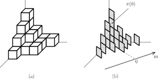
Figure 1: The $3d$ Young diagram (a) and the corresponding sequence of partitions (b).

Diagonal slices of $\pi$ become partitions, as depicted in Fig.1. Denote $\pi(m)$ the partition along the $m$-th diagonal slice, where $m\in\mathbb{Z}$. In particular, $\pi(0)=(\pi_{11},\pi_{22},\cdots)$ is the main diagonal one. This series of partitions satisfies the condition

$$\cdots\prec\pi(-2)\prec\pi(-1)\prec\pi(0)\succ\pi(1)\succ\pi(2)\succ\cdots,$$ (3.6)

where $\mu\succ\nu$ means the interlace relation; $\mu\succ\nu$ $\Longleftrightarrow$ $\mu_{1}\geq\nu_{1}\geq\mu_{2}\geq\nu_{2}\geq\mu_{3}\geq\cdots$.

The hamiltonian picture emerges from the above relations, by viewing a plane partition as evolutions of partitions by the discrete time $m$. Eventually it is described [14] by using $2d$ free complex fermions $\psi,\psi^{*}$. We may separate the relations (3.6) into two parts, each describing the evolutions for $m\leq 0$ and $m\geq 0$. These two types of the evolutions are realized in the $2d$ CFT by using operators $G_{\pm}$ of the forms [14]

$$G_{\pm}=e^{\sum_{k=1}^{\infty}\frac{q^{\frac{k}{2}}}{k(1-q^{k})}J_{\pm k}},$$ (3.7)

where $J_{\pm k}=\sum_{n=-\infty}^{\infty}:\psi_{\pm k-n}\psi^{*}_{n}:$ are the modes of the $U(1)$ current.

Using the free fermion description, one can express the generating function as

$$\mathcal{Z}^{U(1)}_{-i\hbar,i\hbar}(t)=\langle 0|G_{+}Q^{L_{0}}e^{\frac{1}{\hbar^{2}}\sum_{k}t_{k}\hat{\mathcal{O}}_{k}}G_{-}|0\rangle\,,$$ (3.8)

where $L_{0}=\sum_{n=-\infty}^{\infty}n:\psi_{-n}\psi_{n}^{*}:$ is an element of the Virasoro algebra. The loop operators $\mathcal{O}_{k}$ are converted to operators $\hat{O}_{k}$ in the above representation. They are fermion bilinears given by

$$\hat{\mathcal{O}}_{k}=(1-q^{-k})\sum_{n=-\infty}^{+\infty}q^{kn}:\psi_{-n}\psi^{*}_{n}:+1\,,$$ (3.9)

3.2 The integrable structure

The fermion bilinears $\hat{\mathcal{O}}_{k}$ can be regarded as a commutative sub-algebra of the quantum torus Lie algebra realized by the free fermions [6]. The adjoint actions of $G_{\pm}$ on the Lie algebra generate automorphisms of the algebra. Among them, taking advantage of the shift symmetry, the representation (3.8) can be eventually reformulated [6] to

$$\mathcal{Z}^{U(1)}_{-i\hbar,i\hbar}(t)\,=\,\langle 0|\,e^{\frac{1}{2\hbar^{2}}\sum_{k=1}^{\infty}(-)^{k}(1-q^{-k})t_{k}J_{k}}\,\,{\bf g}_{\star}^{5d\,U(1)}\,\,e^{\frac{1}{2\hbar^{2}}\sum_{k=1}^{\infty}(-)^{k}(1-q^{{}^{k}})t_{k}J_{-k}}\,|0\rangle\,.$$ (3.10)

In the above formula, ${\bf g}_{\star}^{5d\,U(1)}$ is an element of $GL(\infty)$ of the form

$${\bf g}_{\star}^{5d\,U(1)}=q^{\frac{W}{2}}G_{-}G_{+}Q^{L_{0}}G_{-}G_{+}q^{\frac{W}{2}}\,,$$ (3.11)

where $W=W_{0}^{(3)}=\sum_{n=-\infty}^{\infty}n^{2}:\psi_{-n}\psi_{n}:$ is a special element of $W_{\infty}$ algebra. The loop operators $\mathcal{O}_{k}$ are converted to $J_{k}$ or $J_{-k}$ in (3.10). These two are actually equivalent in the formula, since ${\bf g}_{\star}^{5d\,U(1)}$ satisfies [6]

$$J_{k}\,{\bf g}_{\star}^{5d\,U(1)}={\bf g}_{\star}^{5d\,U(1)}J_{-k}\,,\hskip 17.07164pt\mbox{for}~{}k\geq 0.$$ (3.12)

Viewing the coupling constants $t$ as a series of time variables, the right hand side of (3.10) is the standard form of a tau function of $2$-Toda hierarchy [15]. However, by virtue of (3.12), the two-sided time evolutions of $2$-Toda hierarchy degenerate to one-sided time evolutions. This precisely gives the reduction to $1$-Toda hierarchy. Thus the generating function becomes a tau function of $1$-Toda hierarchy.

4 Extended Seiberg-Witten geometry of $5d$ theory

We consider the field theory limit of the $U(1)$ theory, which is achieved by letting $\hbar\rightarrow 0$ and amounts to the thermodynamic limit of the melting crystal model. The system is described by the prepotential $\mathcal{F}^{(0)}(t;\Lambda,R)$. From the integrable system viewpoint, $\mathcal{F}^{(0)}$ may be interpreted as a dispersion-less tau function, since the generating function is substantially a tau function of $1$-Toda hierarchy and $\mathcal{F}^{(0)}$ gives the leading order part of the $\hbar$ expansion of $\log\mathcal{Z}^{U(1)}_{-i\hbar,i\hbar}(t)$ To obtain the semi-classical solution, one actually needs to solve the related variational problem, which is reformulated as a Riemann-Hilbert problem. This issue is treated in [10].

4.1 Seiberg-Witten curve of $U(1)$ theory

Let us present the Seiberg-Witten curve for the $U(1)$ theory. We first employ the following curve [16, 17]:

$$\mathcal{C}_{\beta}:\hskip 22.76219pty+y^{-1}=\frac{1}{R\Lambda}(e^{-Rz}-\beta)\,,\hskip 14.22636ptz\in\mathbb{C}\,,$$ (4.1)

where $\beta$ is a real parameter. $\mathcal{C}_{\beta}$ is a double cover of the cylinder $\mathbb{C}^{*}=\mathbb{C}/\frac{2\pi i}{R}$, with a cut $I$ along the real axis on the Riemann sheet. The coupling constants $t$ determine $\beta$ as $\beta=\beta(t)$. To see this, let us introduce a meromorphic differential of the form

$$d\Psi=\Big{\{}1-\frac{1}{2}R^{2}\sum_{k=1}^{\infty}k^{3}t_{k}M_{k}(z)\Big{\}}d\log y\,,$$ (4.2)

where $M_{k}(z)=\sum_{n=0}^{k}d_{k-n}(\beta)e^{-nRz}$. The coefficients $d_{n}(\beta)$ are given in the asymptotic expansion

$$\sqrt{(1-\beta e^{Rz})^{2}-(2R\Lambda e^{Rz})^{2}}=\sum_{n=0}^{\infty}d_{n}(\beta)e^{nRz}\,,\hskip 17.07164pt\Re z\rightarrow-\infty.$$ (4.3)

Finally, solving the Riemann-Hilbert problem, $\beta$ is determined by the condition [10]

$$\oint_{C}zd\Psi=0\hskip 22.76219pt(\mbox{$C$: a contour encircling $I$ anticlockwise}).$$ (4.4)

4.2 Vevs of the loop operators

The vev of the loop operators $\mathcal{O}_{k}$ can be represented by using an analogue of the Seiberg-Witten differential. Eventually, the vev can be organized to the contour integral

$$\frac{\partial\mathcal{F}^{(0)}(t;\Lambda,R)}{\partial t_{k}}=\lim_{\hbar\rightarrow 0}\langle\mathcal{O}_{k}\rangle=\frac{-kR}{2\pi i}\oint_{C}e^{-kRz}dS,,$$ (4.5)

where $dS=S^{\prime}(z)dz$ is an analogue of the Seiberg-Witten differential. $S^{\prime}(z)$ is given by the indefinite integral

$$S^{\prime}(z)=\int^{z}d\Psi\,.$$ (4.6)

The contour integral in the right hand side of (4.5) can be converted to a residue integral. Actually, by using coordinate $Z=e^{-Rz}$, we obtain

$$\frac{\partial\mathcal{F}^{(0)}(t;\Lambda,R)}{\partial t_{k}}=\lim_{\hbar\rightarrow 0}\langle\mathcal{O}_{k}\rangle=kR\,\mbox{Res}_{Z=\infty}\Big{(}Z^{k}dS\Big{)}\,.$$ (4.7)

Acknowledgements

This article is based on a talk presented at the international workshop “Progress of String Theory and Quantum Field Theory” (Osaka City University, December 7-10, 2007). We would like to thank the organizers of the conference for arranging such a wonderful conference. K.T is supported in part by Grant-in-Aid for Scientific Research No. 18340061 and No. 19540179.

References

- [1] N. Nekrasov and A. Okounkov, “Seiberg-Witten Theory and Random Partitions,” hep-th/0306238.
- [2] N. Seiberg and E. Witten, “Electric-Magnetic Duality, Monopole Condensation, and Confinement in N=2 Supersymmetric Yang-Mills Theory,” Nucl. Phys. B426 (1994) 19, hep-th/9407087; Erratum, ibid. B430 (1994) 485; “Monopoles, Duality and Chiral Symmetry Breaking in N=2 Supersymmetric QCD,” ibid. B431 (1994) 484, hep-th/9408099.
- [3] N. A. Nekrasov, “Seiberg-Witten Prepotential from Instanton Counting,” Adv. Theor. Math. Phys. 7 (2004) 831, hep-th/0206161.
-
[4]
A. Marshakov and N. Nekrasov,
“ Extended Seiberg-Witten Theory and Integrable Hierarchy,”
JHEP 0701:104 (2007),
hep-th/0612019.
A. Marshakov, “On Microscopic Origin of Integrability in Seiberg-Witten Theory,” arXiv:0706.2857 [hep-th] - [5] H. Itoyama and K. Maruyoshi, “ Deformation of Dijkgraaf-Vafa Relation via Spontaneously Broken N=2 Supersymmetry I,” arXiv:0704.1060 [hep-th]; “ ibid. II,” arXiv:0710.4377 [hep-th].
- [6] T. Nakatsu and K. Takasaki, “Melting Crystal, Quantum Torus and Toda Hierarchy,” arXiv:0710.5339[hep-th], to appear in Commun. Math. Phys.
- [7] T. Maeda, T. Nakatsu, K. Takasaki and T. Tamakoshi, “Five-Dimensional Supersymmetric Yang-Mills Theories and Random Plane Partitions,” JHEP 0503:056 (2005), hep-th/0412327.
- [8] A. Losev, A. Marshakov and N. Nekrasov, “Small Instantons, Little Strings and Free Fermions,” hep-th/0302191.
- [9] S. Shadchin, “On certain aspects of string theory/gauge theory correspondence,” hep-th/0502180.
- [10] T. Nakatsu, Y. Noma and K. Takasaki, “Extended Seiberg-Witten Theory and Melting Crystal,” to appear.
- [11] H. Nakajima. “Lectures on Hilbert schemes of points on surfaces,” Univ. Lect. Ser. 18, AMS, 1999.
- [12] H. Nakajima and K. Yoshioka, “Lectures on instanton counting,” math.AG/0311058.
- [13] H. Kanno and S. Moriyama, “Instanton Calculus and Loop Operator in Supersymmetric Gauge Theory,” arXiv:0712.0414[hep-th].
- [14] A. Okounkov and N. Reshetikhin, “Correlation Function of Schur Process with Application to Local Geometry of a Random 3-Dimensional Young Diagram,” J. Amer. Math. Soc. 16 (2003) no.3 581, math.CO/0107056.
- [15] K. Ueno and K. Takasaki, “Toda lattice hierarchy,” Adv. Studies in Pure Math. 4, Group Representations and Systems of Differential Equations, 1-95, 1984.
- [16] T. Maeda, T. Nakatsu, “Amoebas and Instantons,” Internat. J. Modern Phys. A 22 (2007) 937, het-th/0601233.
- [17] T. Maeda, T. Nakatsu, K. Takasaki and T. Tamakoshi, “Free fermion and Seiberg-Witten differential in random plane partitions,” Nucl. Phys. B715 (2005) 275, hep-th/0412329.