Simultaneous Absolute Timing of the Crab Pulsar at Radio and Optical Wavelengths

Abstract

Context. The Crab pulsar emits across a large part of the electromagnetic spectrum. Determining the time delay between the emission at different wavelengths will allow to better constrain the site and mechanism of the emission.We have simultaneously observed the Crab Pulsar in the optical with S-Cam, an instrument based on Superconducting Tunneling Junctions (STJs) with $\mu$s time resolution and at 2 GHz using the Nançay radio telescope with an instrument doing coherent dedispersion and able to record giant pulses data.

Aims. We have studied the delay between the radio and optical pulse using simultaneously obtained data therefore reducing possible uncertainties present in previous observations.

Methods. We determined the arrival times of the (mean) optical and radio pulse and compared them using the tempo2 software package.

Results. We present the most accurate value for the optical-radio lag of 255$\pm$21 $\mu$s and suggest the likelihood of a spectral dependence to the excess optical emission asociated with giant radio pulses.

1 Introduction

The Crab pulsar was the first pulsar detected as a consequence of its occasional bright pulses (now known as Giant Radio Pulses) at radio wavelengths (Staelin & Reifenstein staelin:1968 (1968); the first pulsar ever detected was PSR J1921+2153 Hewish et al. hewish:1968 (1968)). Later on pulsations have been detected at optical wavelengths (Cocke et al.; cocke:1969 (1969)) and throughout the electromagnetic spectrum at X-rays and $\gamma$-rays. One feature which is constant over the whole spectrum is the pulsed emission, but the details differ substantially. E.g. the strength of the interpulse, the presence of a pre-cursor to the main pulse (at low radio frequencies) change with wavelength. However, the precise timing of the pulse over many orders of magnitude of energy imposes severe constraints on the emission regions (and mechanism). For example Romani & Yadigaroglu (romani:1995 (1995)) have suggested that the pre-cursor originates at the polar cap, while the pulse and interpulse originate in the outer gap in the magnetosphere, with higher energy pulses being generated at significantly greater heights. This should then be reflected in the timing of the pulses at different energies. Small differences in pulse alignment allow to study the emission regions at relatively small scales (about 10 km per 0.001 phase in case of the Crab pulsar), and precise timing of pulsar light curves throughout the electromagnetic spectrum is thus a powerful tool to constrain theories of the spatial distribution of various emission regions: a time delay most naturally implies that the emission regions differ in position.

In recent years, it has become clear that the main and secondary pulses of the Crab Pulsar (PSR J0534+2200) are not aligned in time at different wavelengths. X-rays are leading the radio pulse by reported values of 344$\pm$40 $\mu$s (Rots et al. rots:2004 (2004); RXTE data) and 280$\pm$40 $\mu$s (Kuiper et al. kuiper:2003 (2003); INTEGRAL data) and $\gamma$-rays are leading the radio pulse by 241$\pm$29 $\mu$s (Kuiper et al. kuiper:2003 (2003); EGRET data. The uncertainty in this value does not include the EGRET absolute timing uncertainty of better than 100 $\mu$s). At optical wavelengths, the observations presented a less coherent picture. Sanwal (1999) has reported a time shift of 140 $\mu$s (optical leading the radio). The uncertainty in this value is 20 $\mu$s in the determination of the optical peak and 75 $\mu$s in the radio ephemeris. Shearer et al. (shearer:2003 (2003)) have reported a lead of 100$\pm$20 $\mu$s for simultaneous optical and radio observations of giant radio pulses. Golden et al. (golden:2000 (2000)) have reported that the optical pulse trails the radio pulse by $\sim$80$\pm$60 $\mu$s. Romani et al. (romani:2001 (2001)) conclude that the radio and optical peaks are coincident to better than 30 $\mu$s, but their error excludes the uncertainty of the radio ephemeris (150 $\mu$s). Oosterbroek et al. (oosterbroek:2006 (2006), hereafter O06) have studied this issue in detail and found an optical lead of 273$\pm$100 $\mu$s. In this paper we will use simultaneous optical and radio observations at 2 GHz to further improve the accuracy of this value.

We also study the possible changes in the peak emission coincident with Giant Radio Pulses (hereafter GP) as previously reported by Shearer et al. (shearer:2003 (2003)).

2 Observations

Table 1: Log of optical and radio observations. All times are in UT. The first two optical observations were performed with a different instrumental setting resulting in different instrumental delays (see text).

Observation	exposure (s)	Start time (yyyy-mm-dd hh:mm:ss)
0001	179	2007-09-16 04:05:49
0002	900	2007-09-16 04:09:05
0003	900	2007-09-16 04:25:58
0004	900	2007-09-16 04:41:03
0005	900	2007-09-16 04:56:09
0006	900	2007-09-16 05:11:14
0007	900	2007-09-16 05:26:19
0008	900	2007-09-16 05:41:25
0009	373	2007-09-16 05:56:30
0013	1800	2007-09-17 04:10:47
0014	1800	2007-09-17 04:41:42
0015	1800	2007-09-17 05:11:48
0016	1100	2007-09-17 05:41:53
Radio 1	3420	2007-09-15 05:17:10
Radio 2	3930	2007-09-16 05:12:50
Radio 3	3960	2007-09-17 05:08:40
Radio 4	3890	2007-09-18 05:04:50

Optical observations were obtained with S-Cam3 (Martin et al. martin:2006 (2006)) mounted on the ESA Optical Ground Station (OGS) telescope on Tenerife on September 16 and 17 2007. For test purposes the first two observations were obtained in the so-called FAST mode of the instrument. This mode only differs in the digital filter used to obtain the pulse shape of the photons. In S-Cam3 each photon gives rise to a bi-polar signal in the detector electronics chain. the zero-crossing of this signal is used to time tag the photon. The instrumental delays in both modes were determined by triggering an LED using a GPS and registering the assigned time of the observed photons (see also O06). The instrumental delay of S-Cam3 amounts to 39.7$\pm$0.5 $\mu$s in the instrumental mode which was used for all but the first two observations, and 14.0$\pm$0.5 $\mu$s for the first two (i.e. “FAST mode”) observations. Note that these values are different from those reported in O06, since a physically different detector array and different instrument modes were used. Observations 0009 and 0016 have a shorter duration than the typical exposure time for the night since they were interrupted because of rising sky background (twilight). Some thin cirrus was present at the end of the first night (starting at around 5:30 UT), while the seeing was somewhat better during the first night compared to the second night.

Radio observations at 2 GHz were performed using the Nançay radio telescope on September 15-18 2007. The observations were done over a bandwidth of 64 MHz (from 2016–2080 MHz) in 16 channels. Data were coherently dedispersed over 4 MHz bandwidth channels (providing 250 ns resolution) using a transfer function in the complex Fourier domain of the recorded voltages (Cognard & Theureau cognard:2006 (2006), Demorest demorest:2007 (2007)). Using a polynomial representation for the expected evolution of the apparent rotational phase of the pulsar, data were folded to produce a profile every minute. A daily profile is built by integration of the 1-minute profiles obtained over the typical 1-hour duration of an observation. During data processing, the instrumentation is able to detect and store shortlived events such as giant pulses known to occur on this pulsar. Radio observations at this high frequency allow to minimize the effect of uncertainties in the Dispersion Measure (DM). For a log of the optical and radio observations we refer to table 1.

3 Analysis and Results

3.1 Optical TOAs

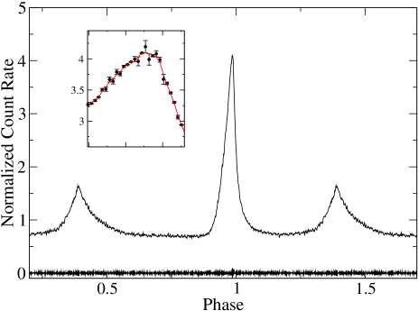
Figure 1: The pulse profile template used for obtaining the TOAs. The profile shown is the modestly smoothed profile (see text) which at this scale is indistinguishable from the unprocessed data. In the zoom-in the difference between the data points (circles with error bars) and the smoothed data (line) is shown for the peak where the differences are largest. At the bottom of the main plot the difference between the smoothed and non-smoothed data is shown.

The analysis of the optical data consisted of searching for the best local period by using a profile-folding technique for each S-Cam observation. Since these observations are relatively short (up to 1800s) we did not take into account the period derivative nor did we perform any barycentering on the time stamps. The data was then folded on the best local period, using the midpoint of the observation as the epoch. This resulted in 13 profiles, one for each observation. A template profile was constructed. This template was created by applying a barycentric correction to the time stamps of the photons and folding on phase (i.e. calculating the phase of every photon using an epoch and period and summing to obtain a phase histogram) using the best period determined by folding the data on a range of trial periods and maximizing the $\chi^{2}$ with respect to the mean. All data were used, except the two first observation, since they are obtained in a different instrumental mode. A cross-correlation between every observation and the template profile was performed and the delay/lead was determined by fitting a Gaussian around the peak of the cross-correlation curve. The time of arrival of each average pulse profile was then assigned to the midpoint of each observation. These TOA’s were corrected for the instrumental delay of S-Cam (14.0$\pm$0.5 $\mu$s for the first two observations, 39.7$\pm$0.5 $\mu$s for the remainder, see Sect. 2). Using the cross-correlation technique the most significant contribution to the uncertainty in the TOA is the uncertainty in the determination of the peak of the template profile, which amounts to 18 $\mu$s. This uncertainty was determined by fitting the data points with a Gaussian in a 0.01 wide phase range around the peak. This phase range was determined iteratively and choosen symmetrically around the peak (see also O06). The uncertainty represents the 1 $\sigma$ uncertainty on the peak position ($\Delta\chi^{2}=1$). This uncertainty is larger than the uncertainty introduced by the cross-correlation since for the cross-correlation the whole profile is used. The individual uncertainties from the cross-correlation are an estimated 1.4–3.3 $\mu$s. The value of 18 $\mu$s can be considered as a systematical error on all the indivual optical points, since they are all determined using the same template profile.

In order to test whether some of the scatter in arrival times was caused by the presence of noise in the template profile we constructed a template profile using all data (except the first two observations) which was modestly smoothed by a Savitzky-Golay filter (see Fig. 1). The filter was constructed using 4 forward and 4 backward data points and degree 4 (see Press et al. press:1992 (1992)). This almost did not affect the results: arrival times did not change by more than 4.3 $\mu$s and the change was typically less than 2 $\mu$s in a seemingly random way. This implies that the obtained time shift does not depend on some modest smoothing of the template pulse profile.

3.2 Radio TOAs

The radio time of arrivals (TOAs) were derived for each day of observations yielding 4 TOAs. Each TOA was obtained by doing a cross-correlation of each daily profile with a mean profile obtained by integration over many months of observation. This cross-correlation gives a time and a uncertainty ranging from 3 to 8 $\mu$s. The relatively low signal-to-noise ratio (around 20) for the daily profiles explains the limited accuracy of the TOA determinations. The reference point in the mean profile was chosen to be the phase bin with highest radio flux. Given the signal-to-noise ratio and the width of the phase bins, we estimate that this introduces an uncertainty of 8 $\mu$s which affects the ensemble of radio TOA in an identical way (and does not disappear when averaged over multiple TOAs).

The determination of the radio TOAs included the Nançay instrumental delay. This delay was estimated from several observations of the millisecond pulsar J1824-2452 done with the Green Bank and the Nançay radiotelescopes at the same epoch. A careful analysis of the mean profiles obtained with the two similar instrumentations installed at Green Bank and Nançay (both Astronomy Signal Processor -ASP-, Demorest, demorest:2007 (2007)) give a relative offset of 7.0$\pm$0.4 $\mu$s. Knowing accurately the Green Bank instrumental delay (which amounts to 15.74 $\mu$s; Demorest, demorest:2008 (2008)), we can derive the Nançay instrumental delay as 8.7$\pm$0.4 $\mu$s.

3.3 Giant radio pulses and DM determination

Figure 2: Example of a giant pulse detected on Sept 17th with the Nançay radiotelescope. Total intensity is plotted for every 4 MHz channels with a resolution of 250 ns. Duration of this giant pulse is of the order of 2 $\mu$s.

Accurate determination of DM variations is usually done from TOAs obtained at two different frequencies, as much separated as possible in order to maximize the effect of the differential dispersion delay to measure. However, as shown by Ramachandran et al. (ramachandran:2006 (2006)), highly frequency-dependent multipath propagation in the turbulent interstellar medium produces huge variations of the space (cigar shape like) within which the radio waves senses the electron density. TOAs obtained at very different frequencies did not see exactly the same electron density and should not be used to derive a highly reliable Dispersion Measure value. Using frequencies as close as possible tends to remove this effect but then TOAs determination must be much better to compensate. As Giant Pulses TOAs are characterized by very short bursts of radio emissions suitable for a very good TOA determination, we should be able to use them even on limited frequency span to determine unbiased DM variations. For example, a differential delay between 2016 and 2080 MHz known at 0.5 $\mu$s gives roughly the same DM uncertainty as a 10 $\mu$s accuracy between 1400 and 2050 MHz.

Figure 3: The DM value determined from the Nançay GP data. Displayed are the nightly mean values.

We have determined the DM value from the Nançay data alone in the following way: each GP (an example is shown in Fig. 2) which was detected in more than 14 channels (among the 16 available, using a 15 sigma threshold for each channel) was dedispersed with different DM values and integrated in frequency to produce a 56 to 64 MHz total bandwidth profile. Based on the fact that a good DM value will tend to properly align the individual GPs and thus maximize the amplitude of the integrated profile, this maximum amplitude was kept for each trial DM and a gaussian fit was done on those maximum amplitudes to find the best DM. An average of the numerous DM obtained for a given observation (one per single GP event) provides us with a nightly DM value (see Fig. 3). Uncertainties are estimated from the rms of the different DM values obtained each night. The overall average value over the 69 DM values obtained over 4 nights is 56.7740 pc.cm^-3 and again an uncertainty of 0.005 is estimated (from the rms over the 69 individual values).

3.4 Optical-radio lag

We determined an improved solution to the $\nu$ and $\dot{\nu}$ starting from the Jodrell Bank ephemeris to the TOAs of the mean pulse using the Nançay radio data. While the fit to the 4 data points is not very constraining, it establishes a reliable baseline against which the optical TOAs can be compared. The obtained values are $\nu=29.755351174(9)$s^-1, and $\dot{\nu}=-3.727(6)\times 10^{-10}$s^-2 (for a fixed value of $\ddot{\nu}$ of $3.72\times 10^{-22}$s^-3). The dispersion measure was fixed at the value reported above of 56.7740 pc cm^-3.

The OGS geocentric coordinates used in the reduction (within tempo2) are (X,Y,Z) = (5390280.91, -1597890.59, 3007083.48). These coordinates were obtained from the reading of two different GPS units (see O06). The obtained optical TOAs were then used in the tempo2 analysis package (Hobbs et al. hobbs:2006 (2006)), together with the radio TOAs. The radio and optical data points were fit together allowing for an offset between the radio and optical. Since a comparison of arrival times is made at (almost) the same time, this procedure is not substantially affected by e.g. uncertainties in the pulsar position (proper motion) or uncertainties in e.g. frequency and derivatives.

In Fig. 4 the results of this analysis are displayed: an offset of 255$\pm$4 $\mu$s between the radio peak and the optical peak. The uncertainty in this value is purely the statistical uncertainty in the best-fit value for an offset between the radio and the optical measurements. This value does not take into account uncertainties in the DM values, which could be of the same order. A difference in the DM value of 0.005 pc cm^-3 (more than a typical month-to-month variation, see Fig. 5) will result in a time difference at 2 GHz of $\sim$6 $\mu$s. We therefore assume an uncertainty of 6 $\mu$s as a result of uncertainties in the DM value. This uncertainty in time is smaller than quoted by other authors (e.g. Lyne et al. lyne:1993 (1993)), since our radio observations have been obtained at a higher frequency which is substantially less affected by timing delays due to scattering.

Figure 4: Comparison of radio and optical results. At the bottom a zoom-in on the optical data points only is presented. Plotted error bars represent 1 $\sigma$ uncertainties.

Adding all of the above uncertainties (18 $\mu$s from the optical template, 8 $\mu$s from the radio template, 6 $\mu$s from DM uncertainty, 4 $\mu$s from the fit to the offset between the radio and optical TOAs) linearly we obtain a total uncertainty of 36 $\mu$s. This is likely to be an overestimate of the total uncertainty since all individual deviations have to be in the same direction to end up at this value. Adding all uncertainties in quadrature yields a final uncertainty of 21 $\mu$s.

From Fig. 4 we conclude that the variation in the optical-radio delay is substantially larger than the individual uncertainties on the TOAs (which are between 1.4 and 2.1 $\mu$s, 1$\sigma$). The average value of the delays obtained during the first and second night differ by 6 $\mu$s (only 1.4 $\mu$s when one excludes the deviant point in the second night). The observed scatter during the first night and the possible difference between the two nights, suggests that small variations (less than about 10 $\mu$s) exist. For this relative comparison the uncertainties introduced by determining phase zero on both the radio and optical templates (which each amount to 8 $\mu$s) should not be considered, since they affect all data points in the same way. We consider it unlikely that this night-to-night variation is solely caused by variations in the DM, since a variation of $\sim$1 times that of typical monthly variations is needed in 1 day. Variations in the peak position on time scales of days and shorter are studied in more detail by Karpov et al. (karpov:2007 (2007)), who find, during one observation, variations at the $\sim$150 $\mu$s-level.

Figure 5: The recent (past 1000 days) history of the dispersion measure towards the Crab pulsar (data taken from Lyne et al. lyne:2007 (2007)). The data points are monthly values. The time of our observations is indicated by an arrow. The difference between the Nançay DM value and the value plotted here is less than 2 $\sigma$ (offset is 0.008 while uncertainty is 0.005 for both determinations). As the frequency spans used for these two derivations are not the same (610-1400 MHz for Jodrell and 2018-2080 MHz for Nançay), the difference is acceptable (see text).

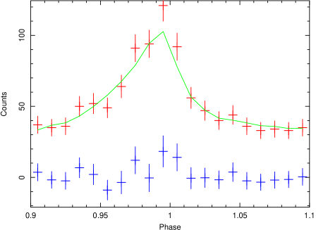
Figure 6: A comparison of the optical pulse profile obtained coincident with a Giant radio Pulse in red and a reference profile in green (see text). The difference between the two is also displayed.

3.5 Giant radio pulses and optical

In total 927 Giant radio pulses were detected during the radio observations. The rate of GPs was much higher during the second night where we have optical data (on average 1 per 6.6 s) than the first night (1 per 29.5 s).

Following the method by Shearer et al. (shearer:2003 (2003)) we have selected the optical data coincident with Giant Pulses (GPs) detected in the radio observations. The barycentric arrival times of the GPs were computed using tempo2, while the event time tags were corrected using our barycentering code. We checked that these corrections are consistent to better than 15 $\mu$s and that therefore this procedure provides the required accuracy. We find, in total, 603 GPs coincident with optical data. We made sure that these GPs occurred near the main peak of the profile and selected data half a phase range before and half a phase range after the main peak (in the radio). The data was then folded to obtain a pulse profile coincident with radio GPs. A reference profile was also constructed from data spanning 80 cycles around (but not including) this cycle. This was done since changes in sky background and airmass force us to select data close to the cycle coincident with the GP. Several different ranges were tried and all gave similar results, with obviously better statistics as the number was increased. We settled for 80 cycles, since this gives a very good reference profile and yet it still only spans 2.7 s of data. We ensured that no optical data was missing during these periods (e.g. at the end of an observation). We present the obtained results in Fig. 6. As can be seen from this figure no clear excess is present. Depending on the choice of phase range this excess amounts to about $\sim 2.1\sigma$. We view this a confirmation of the result of Shearer et al. (shearer:2003 (2003)) and shows that their dataset has a much better statistical quality given the longer exposure times and larger telescope aperture.

3.6 Wavelength dependence of the delays

In order to investigate whether we are able to detect a delay between the pulse profiles obtained at different wavelengths we divided the photons obtained during the observations described above in three adjacent bands, each containing approximately the same number of photons, using the intrinsic energy resolution of S-Cam. The wavelength boundaries of the three bands were: 3920–5490 Å, 5490–6330 Å, 6330–8230 Å. We then created the folded profiles per observation and did the crosscorrelation with the smoothed profile (which was obtained using all photons) as described above. The results are displayed in Fig. 7. While the quality of the data does not seem to justify drawing strong conclusions, a linear fit to the datapoints reveals that the slope in the delay is -5.9$\pm 1.9$ $\mu$s/1000 Å, which seems to indicate that the blue photons arrive, averaged over phase, slightly earlier than the red photons. A similar result is obtained when only the main peak part of the pulse profile is used for this analysis. It is important to realize that this is only a statement about the phase-averaged arrival times of photons: the full width at half-maximum (FWHM) of the pulse peak is known to decrease with decreasing wavelength (Percival et al. percival:1993 (1993), Eikenberry et al. eikenberry:1997 (1997), Sollerman et al. sollerman:2000 (2000)). This trend is also evident in our data. Together with the assymmetry in the profile the decrease in FWHM with decreasing wavelength will lead to an average time shift. Close inspection of our profiles in colour suggests that the profile rises slightly earlier in the blue band, which could yield the result present above. Furthermore the separation between the main and secondary peak is smaller in the UV than in the optical (Percival et al. percival:1993 (1993)). In essence this shows the limitation of using the cross-correlation method: it is only possible to obtain a proper time shift if the profile and template are identical in shape. Any other method (e.g. fitting around the peak) will also be affected by the assymetry of the profile and will give similar results.

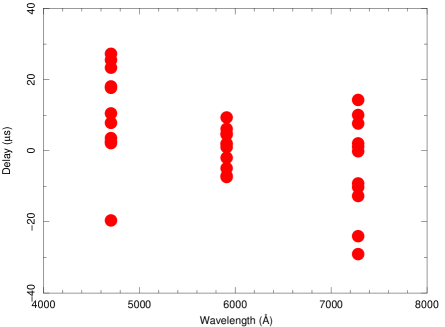
Figure 7: The delay between photons in different energy bands. Wavelengths indicate the center of the three bands (not the average energy of the photons).

4 Discussion and Conclusions

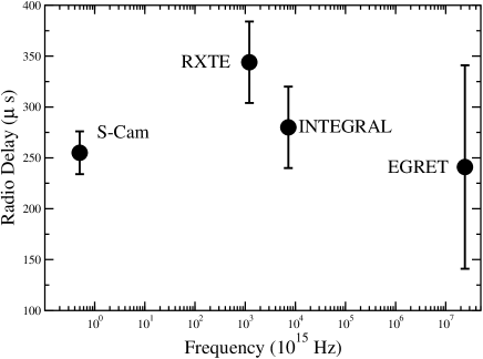
Figure 8: The radio delay with respect to other frequencies. The S-Cam data point is presented in this paper, the RXTE value is from Rots et al. (rots:2004 (2004)), the INTEGRAL and EGRET points are taken from Kuiper et al. (kuiper:2003 (2003)). We have added a 100 $\mu$s error bar to the EGRET value, because of uncertainties in the EGRET absolute time calibration (see Kuiper et al. kuiper:2003 (2003)).

We have performed simultaneous observations of the Crab pulsar in the optical (3500–8200 Å) and radio (2 GHz). The results provide the current best estimate of the optical lead (with respect to the radio peak) of 255$\pm$21 $\mu$s. The two major contributions to the uncertainty are the determination (or definition) of the peak in the optical, since the profile is asymmetric, and uncertainties in the DM value which translate into significant uncertainty in the correction of the radio data. Additionally a true jitter in the optical peak on different time scales might take place with an amplitude of 5–10 $\mu$s. However, our value is an order of magnitude more precise than determined by O06 and fully consistent with the value reported there. The close match with their value (273$\pm$100 $\mu$s) must be fortuitious given the large uncertainties on the values, and can be considered a statistical coincidence. A comparison with previous results can be be found in O06, however due to the increased precision we can now conclude that the result of Shearer et al. (shearer:2003 (2003)), an optical lead of 100$\pm$20 $\mu$s, is not consistent with our result. Together with the result of Golden et al. (golden:2000 (2000)), an optical delay of $\sim$80$\pm$60 $\mu$s, which was already inconsistent with the results presented in O06, this raises the possibility of a long-term change in the radio-optical difference.

From a plot of the radio delay throughout the electromagnetic spectrum (see Fig. 8) it appears that this delay is approximately constant over more than 7 orders of magnitude. We note that the non-optical results have been derived from a comparison with, non-simultaneous Jodrell Bank observations, which results in larger error bars. This near-constancy of the delay with respect to the radio profile implies a similar emission mechanism and emission location from the optical to $\gamma$-rays. This is indeed the case in modern models by e.g. Takata & Chang (takata:2007 (2007)).

Our results for the stability of the pulse profile (differences of up to $\sim$10 $\mu$s on a time scale of a day and even smaller variations on a time scale of less than a day; see Fig. 4) are not consistent with the results from Karpov et al. (karpov:2007 (2007)) who present variations of up to $\sim$150 $\mu$s in a fraction of a day. However, this variation is only present in a small part of their data set (December 2005 and January 2006), while the remainder of their data (obtained in December 1994 and 1999, and November 2003) do not show substantial variations. This suggest that the behaviour observed in December-January 2005/2006 is an anomaly and that night-to-night variations in the Crab optical peak positions amounts to at most $\sim$10 $\mu$s.

Our value for the time delay between red and blue photons of -5.9$\pm 1.9$ $\mu$s/1000 Å can be compared to the results of Sanwal (sanwal:1999 (1999)) who found a delay between the R and U band of -10$\pm$4 $\mu$s and Golden et al. (golden:2000 (2000)) who found that the peaks in B and V are coincident within 10 $\mu$s. Taken together these three measurements indicate a small delay between blue and red photons. However changes in the FWHM of the pulse profile and the assymmetry of the profile and possible differences in the separation between the main and secondary peak make an interpretation complex.

Current models for high-energy pulsar emission (e.g. Dyks & Rudak dyks:2003 (2003)), describe the peaks as caustics: special relativity effects (aberration of emission directions and time of flight delays due to the finite speed of light) cause photons emitted at different altitudes to pile up at the same pulse phase. It is difficult if not contrived to imagine how caustics originating from the trailing edge extending along the full length of the open field lines within the magnetosphere could produce phase bunching yielding a common main peak cusp spanning 7 orders of magnitude in photon energy from incoherent synchrotron emission, and less than 1% in phase difference from coherent radio emitting sources, spanning in this case some 12 orders in photon energy. As such arguments are usually presented in the context of outer gap or slot gap model formalisms, these new results argue strongly for a localised source for the observed multiwavelength emission from the Crab pulsar.

That the radio and higher energy emission process are in someway linked is not in doubt, following on from the optical-GP association originally shown by Shearer et al. (shearer:2003 (2003)). Our confirmation of an excess, albeit at low significance further strengthens the connection between these energy bands. Variations in the optical emission correlated with GPs have been argued to be a consequence of local density enhancements to the plasma stream (Shearer et al. shearer:2003 (2003)). Recent studies of GPs from the Crab have indicated that these can and do originate as short-lived ($\sim$ ns), narrowband nanoshots, which have been argued to have their origin in strong, highly localised plasma turbulence (Hankins & Eilek, hankins:2007 (2007)). That there is no change in phase or shape of the Crab’s optical light curve morphology during a GP associated event, just flux, requires an extended region of plasma turbulence to produce the same phase-bunching effect following the caustic model $ansatz$, which is clearly implausible. The measured time delay across the optical bands represents $\leq$ 3.0 $\times$ 10^-4 of phase, with some evidence of a jitter in the optical peak across several time scales occuring with a similar variation in terms of phase. Again, these effects are not associated with any measurable change in incident flux. Assuming a constant emission source, localised geometric constraints represent the most likely cause of such observational effects. Together these interpretations merit some revision of the fundamental approaches to modeling the Crab pulsar’s emission processes, and there may be some use in trying to geometrically constrain emission regions within the magnetosphere first, and then address the local physical conditions that are consistent with the data we have available to us - rather than the other way round.

Finally the anticipated detection of excess optical emission associated with GPs extrapolating from the work of Shearer et al. (2003) was expected to be $<1\sigma$ prior to our observations, so its marginal detection is somewhat surprising. We note that our passband ($\sim$3500–$\sim$8000 Å) is quite different from the passband (6000–7500 Å) of Shearer et al. (shearer:2003 (2003)) and might result in different results depending on the spectrum of the “excess” optical emission. If our observed excess had been significant we could have constructed the optical spectrum obtained when a GP occurs and compare it with the reference spectrum when no GP is present. This is possible by using the intrinsic energy resolution of S-Cam (each photon is tagged with a time stamp, but also its energy, Martin et al. martin:2006 (2006)). Such an approach could reveal the spectrum of the excess emission and consequently would impose important further constraints on the emission mechanism. We regard the acquisition of deeper coincident radio-optical data as critically important to confirm the spectral dependence of such an excess.

- (1) Cocke, W.J., Disney, M.J., Taylor, D.J., 1969, Nature, 221, 525
- (2) Cognard, I., Theureau, G., 2006, On the Present and Future of Pulsar Astronomy, 26th meeting of the IAU, Joint Discussion 2, Prague, Czech Republic, JD02, 36
- (3) Demorest, P.B., 2007, PhD thesis, University of California, Berkeley
- (4) Demorest, P.B., 2008, personal communication
- (5) Dyks, J., Rudak, B., 2003, ApJ, 598, 1201
- (6) Eikenberry, S.S., Fazio, G.G., Ransom, S.M., Middleditch, J., Kristian, J., Pennypacker, C.R., 1997, ApJ, 477, 465
- (7) Golden, A., Shearer, A., Redfern, R.M., et al. 2000, ApJ, 363, 617
- (8) Hankins, T.H., Eilek, J.A., 2007, ApJ, 670, 693
- (9) Hewish, A., Bell, S.J., Pilkington, J.D., Scott, P.F., Collins, R.A., 1968, Nature, 217, 709
- (10) Hobbs, G.B., Edwards, R.T., Manchester, R.N., 2006, MNRAS, 369, 655
- (11) Kanbach, G., Słowikowska, A., Kellner, S., Steinle, H., 2005, Astrophysical Sources of High Energy Particles and Radiation, 801, 306
- (12) Karpov, S., Beskin, G., Biryukov, A., Debur, V., Plokhotnichenko, V., Redfern, M., Shearer, A., 2007, Ap&SS, 308, 595
- (13) Kuiper, L., Hermsen, W., Walter, R., Foschini, L., 2003, A&A, 411, L31
- (14) Lyne, A.G., Pritchard, R.S., Graham-Smith, F., 1993, MNRAS, 265, 1003
- (15) Lyne, A.G., Jordan, C.A., Roberts, M.E., 2007, Crab Monthly Ephemeris available on http://www.jb.man.ac.uk/~pulsar/crab.html
- (16) Martin, D.D.E., Verhoeve, P., Oosterbroek, T., et al., 2006, Proc. SPIE Vol 6269
- (17) Oosterbroek, T., de Bruijne, J.H.J., Martin, D., Verhoeve, P., Perryman, M.A.C., Erd, C., Schulz, R., 2006, A&A, 456, 283 (O06)
- (18) Percival, J.W., Biggs, J.D., Dolan, J.F, et al., 1993, ApJ, 407, 276
- (19) Press, W.H., Teukolsky, S.A., Vetterling, W.T., Flannery, B.P., 1992, Numerical recipes in FORTRAN. The art of scientific computing, Cambridge University Press
- (20) Ramachandran, R., Demorest, P., Backer, D.C., Cognard, I., Lommen, A., 2006, ApJ, 645, 303
- (21) Romani, R.W., & Yadigaroglu, I.A., 1995, ApJ, 438, 314
- (22) Romani, R.W., et al. 2001, ApJ, 563, 221
- (23) Rots, A.H., Jahoda, K., Lyne, A.G., 2004, ApJ, 605, L129
- (24) Sanwal, D., 1999, Ph.D. thesis, Univ. Texas at Austin
- (25) Shearer, A., Stappers, B., O’Connor, P., et al. 2003, Science, 301, 493
- (26) Sollerman, J., Lundqvist, P., Lindler, D., Chevalier, R.A., Fransson, C., Gull, T.R., Pun, C.S.J., Sonneborn, G., 2000, ApJ, 537, 861
- (27) Staelin, D.H., Reifenstein, E.C., 1968, Science, 162, 1481
- (28) Takata, J., Chang, H.-K., 2007, ApJ, 670, 677