Dependence of vertical cutoff rigidities and magnetospheric transmission on empiric parameters

Abstract

Using dynamic paraboloid model of Earth’s magnetosphere, a large set of particles’ trajectory computations was performed. Based on its result, the numerical algorithm for calculating effective cutoff rigidity dependence on empiric parameters has been developed for further use in magnetospheric transmission calculations.

keywords: cutoff rigidity, dynamic paraboloid model, magnetospheric transmission, radiation condition on LEO

1 Introduction

Radiation condition onboard LEO spacecrafts is determined, particularly, by the charged particles penetrating from outside of the magnetosphere. The measure of such a process in any given near-Earth space location is a local geomagnetic cutoff rigidity value. In this work we assume, that ”cutoff rigidity” phrase denotes an effective vertical cutoff rigidity ($R_{eff}$), which value is gained from calculated discrete penumbra structure by ordinary technique using white spectra (for example,  [1]).

It is well known, that magnitude of $R_{eff}$ and penetration boundaries’ position depend on local time and different magnetospheric condition-related parameters  [2, 3, 4, 5, 6, 9, 10]. Cutoff rigidity value’s variations can be measured in experiments or obtained by some type of computation using Earth’s magnetosphere model. However, usual method for $R_{eff}$ calculation is based on resource consuming trajectory computation technique  [7, 8].

In this work we offer the method to calculate $R_{eff}$ with accounting for local time and main empirical parameters, that characterizes magnetospheric condition, in any point of near-Earth’s space. For the applications where $R_{eff}$ calculation is often needed (e.g. transmissions for LEOs) our method provides a huge speedup in comparison with direct trajectory computations. The only things needed for the method are the IGRF rigidity in exploring point and rigidity attenuation  [12] quotient’s dependence on empirical parameters. The first one can be obtained using interpolation in $R_{eff}^{IGRF}$ tabulated data (see, for example,  [11, 13]), which is regularly updated for coming epochs. And the second can be obtained only once by using particle trajectory computations in corresponding numerical magnetospheric model. In our case the dynamic paraboloid model  [16, 17, 18] of Earth’s magnetosphere was chosen for solution of the problem.

2 Cutoff rigidity calculation scheme

We have adopted in our work the cutoff rigidity attenuation formalism  [12, 13], which has already successfully applied  [15] for transmission calculations using Tsyganenko-89  [14] model. The rigidity attenuation quotient $\Delta$ in our case is calculated as

$$\Delta^{model}=R_{eff}^{model}(quiet)/R_{eff}^{model}(disturbed)$$

where $R_{eff}^{model}(quiet)$ value corresponds the set of model parameters for non-disturbed magnetosphere condition, and $R_{eff}^{model}(disturbed)$ is correspond to some set of varied parameters regarding to quiet ones.

As it was wordlessly postulated in  [12], the $\Delta$ dependence on point’s geographical position might not be taken into account because it is relatively small. Generally, it seems to be true at least for $R\gtrsim 0.6$ GV with good enough accuracy (error’s order is about percents even for lowest $R$ in this range). Hence, the approach of calculating a world-wide $R_{eff}$ grid can be essentially simplified.

The algorithm we propose for obtaining $R_{eff}^{model}(LT,parameters)$ in given point contains 3 stages:

• Calculating $R_{eff}^{IGRF}$ for the given point; for practical needs, the interpolation in pre-calculated grid for some altitude $H_{0}$ is often used, it is especially easy when large amount of results is needed quickly. The formula

  $$R_{eff}^{IGRF}(H)=R_{eff}^{IGRF}(H_{0})\cdot\left(\frac{r_{E}+H_{0}}{r_{E}+H}\right)^{2}$$

  can be applied to transform $R_{eff}^{IGRF}$ value to new altitude $H$.

• Calculating a model-dependent cutoff rigidity attenuation quotient
  $\Delta^{model}(R_{eff}^{IGRF},LT,parameters)=R_{eff}^{model}(quiet)/R_{eff}^{model}(R_{eff}^{IGRF},LT,parameters)$ by interpolation in pre-calculated $R_{eff}^{model}$ database (or by extrapolation if $R_{eff}^{IGRF}$ value is out of applied basic $R_{eff}^{IGRF}$ array, see Appendix)

• Computing the resulting value $R_{eff}^{model}=R_{eff}^{IGRF}/\Delta^{model}(R_{eff}^{IGRF},LT,parameters)$

Table of $R_{eff}^{IGRF}$ values for some given altitude $H_{0}$ is needed to be renewed every 5 years with new IGRF epoch coming. Values $R_{eff}^{model}(quiet)$ were obtained by trajectory computations using dynamic paraboloid model with parameter set $[7,380,0,0,5,-3,1]$ (sequence of variables is according to table 1 below). To compute $R_{eff}^{model}$ database which is intended to provide dependence of $\Delta^{model}$ on parameters and local time $LT$, we used the varying of all model parameters in wide enough ranges, comprising extreme, quiet and ”anti-extreme” parameter sets. The multidimensional grid, applied for this calculation, is presented in table 1.

Table 1: The applied parameter grid.

$\rho$	0.5	2	8	20
$v$	400	700	1200	2000
$Dst$	-460	-150	-50	0
$AL$	-2000	-800	-200	0
$B_{x}^{IMF}$	-40	-10	5	20
$B_{y}^{IMF}$	-25	-5	20	50
$B_{z}^{IMF}$	-50	-20	5	30

Values at the edges of this grid were obtained (approximately) from  [19]. All calculations were performed for local time values $3,9,15$ and $21$ hours. Technical details of calculations are summarized in Appendix.

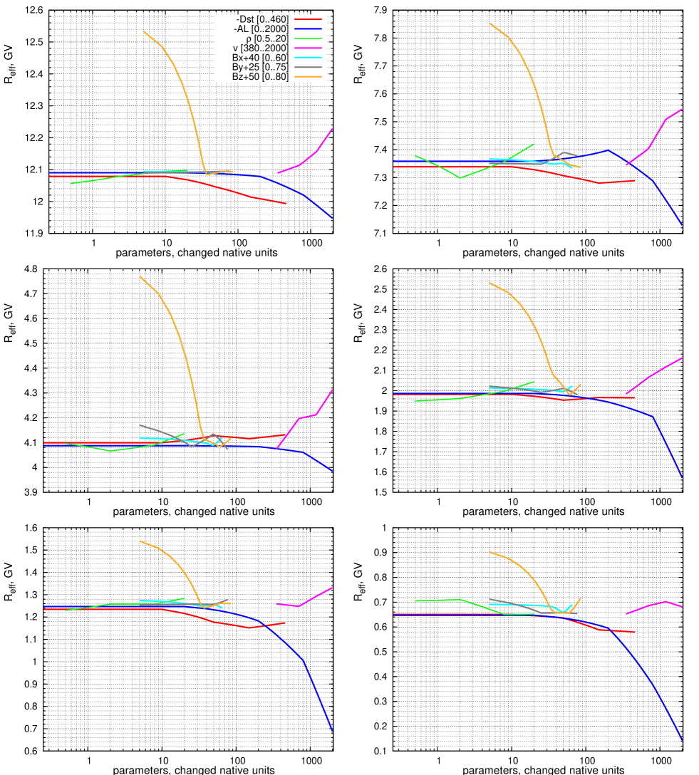
Figure 1: Partial dependencies of $R_{eff}$ on model parameters for six explored points.

Let us now demonstrate some results of cutoff rigidity dependence on local time and model parameters, that have been computed using presented technique.

Fig.1 gives an opportunity to weigh deposit of every model parameter in resulting $R_{eff}$ value for all points of noted above set. Such case of partial dependencies is obtained by fixating all parameters as quiet and excepting the given one. Note, that the role of $Dst$ as $R_{eff}$ depression factor wanes with decreasing of $R_{eff}$, but the $AL$ one rises rapidly. The weight of $B_{x}^{IMF}$ and $B_{y}^{IMF}$ seems to be not important for $R_{eff}$ values, at any hand, in presented case of quiet basic values, because they result in $R_{eff}$ changes that are comparable with the value of applied rigidity step size (see Appendix). Contrary, decrease of $B_{z}^{IMF}$ effects in huge $R_{eff}$ grow (see also fig.2). The effect of $\rho$ and $v$ here is clear but of moderate magnitude.

Fig.2 shows family of $R_{eff}$ daily variations for three points having normal cutoff values of different order. For the first picture there are some hours where $R_{eff}$ is negligibly small, so such a point can be accessible for particles of any rigidity. The middle picture demonstrates the effect of $B_{z}^{IMF}$ ”anti-extreme” setting, leading not only to very high $R_{eff}$ mean values (for this case), but also to the translocation of curve’s maximum for time axis’s positive direction. The upper curve on the most right part of Fig.2 exhibits the insufficiency of applied step size for penumbra calculation (see Appendix), leading to the underestimation of $R_{eff}$ value for $LT=9$, which causes an ambiguous interpolation results. However, this effect is rare and too weak to affect resulting transmission, for which calculating presented method was created.

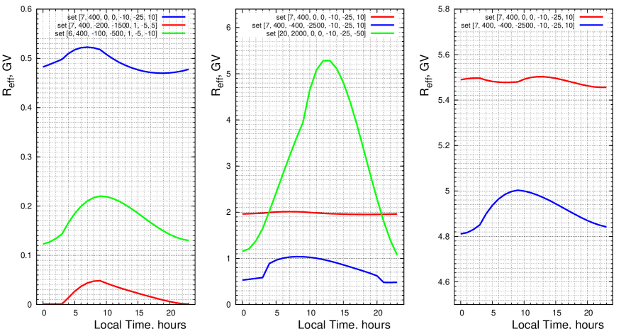
Figure 2: Dependencies of $R_{eff}$ on local time and model parameter set for three points with $R_{eff}^{model}(quiet)$ values 0.49 GV (left), 1.98 GV (middle) and 5.48 GV (right).

A ”gnarlyness” of some presented curves is due to effect of scarce grid, currently imperfect interpolation procedure and scale. It is does not sufficiently affect the results of applications where much of $R_{eff}$ values to be calculated, because interpolation uses many $R_{eff}^{model}$ values and their errors (which are of order of $R$ step size) are to be evened. Extrapolating parameter values to out of grid (but not very far) is also possible and seems to be correct enough to get reliable result.

3 Transmission functions for LEO missions

Magnetospheric transmission functions are directly connected with such tasks as LEO radiation conditions evaluating and the interpretation of orbital experiment results [21]. Because of their importance, it is necessary to be able to account for more empiric factors that affecting transmission. Here we’ll give some examples of calculated magnetospheric transmission functions for several (quiet, disturbed and very extreme) model parameters sets for ISS-like orbit, obtained using presented technique. The essential note is that, unlike Tsyganenko models, the paraboloid one is primordially intended to describe even very extreme conditions, as it is not internally limited by experimental data arrays. Fig.3 presents some modeled transmissions for $H=450$ km $i=51.7^{o}$ circular orbit under different conditions for long mission duration, where all localities are averaged and transmission curve became smoothed. In comparison with additionally figured transmission, obtained by Tsyganenko-89 (T89) model with $Kp=6$, it is obviously seen that the paraboloid model gives unapproachable for T89 results in modeling most extreme conditions.

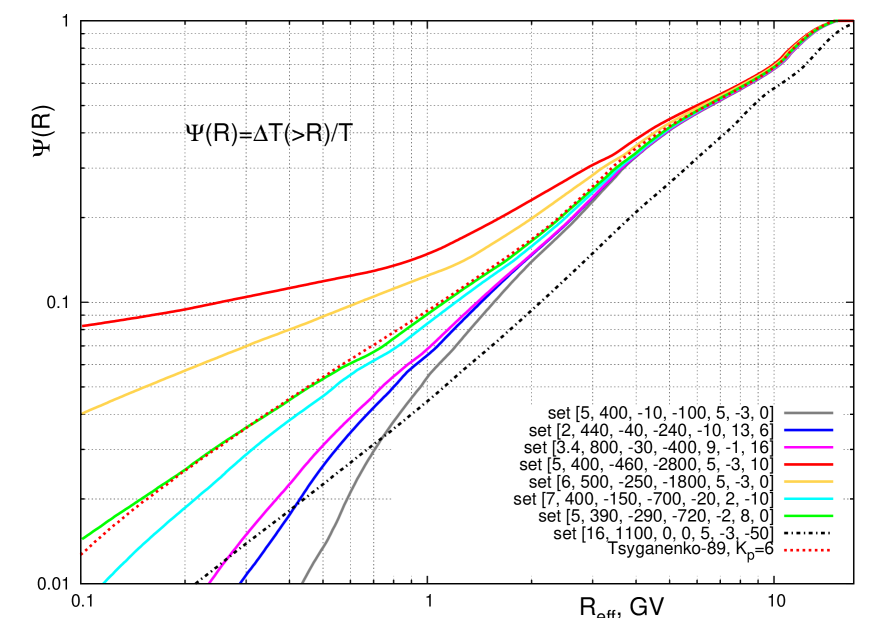
Figure 3: Magnetospheric transmission $\Psi(R)$ for different conditions, obtained according to paraboloid model with using presented technique. Tsyganenko-89 transmission for $Kp=6$ is also figured here for comparison. Note also the standing out of all ”anti-extreme” case.

4 Conclusion

The method we have developing is intended for applications using intensive geomagnetic cutoff calculations, first of all for express magnetospheric transmission calculation for given LEO missions, even under changing magnetospheric conditions during flight. Test $R_{eff}$ and transmission calculation, based on the presented technique, is available online by URL http://dec1.sinp.msu.ru/~vovka/riho (a simplified version, where transmission calculation is allowed for only static conditions and circular orbits).

Current version of the method uses the IGRF rigidity values table as basic (in step 1 of scheme), although it seems that the best choice would be to apply some other world basic grid, for example, one directly calculated $R_{eff}^{model}(quiet)$ table with using paraboloid model. Nevertheless, it does not understate the attenuation quotient methodology itself, because its drawback in our case is only correspond to relatively small systematic inaccuracies between conditional ”quiet” $R_{eff}^{model}$ values and IGRF ones.

Appendix. Technical details

Here we summarize technical moments that are related to the performed $R_{eff}^{model}$ trajectory calculations with using paraboloid model.

Vertically directed protons were test particles for reverse trajectory calculations of penumbra. Fourth order integration scheme was used for it, with accounting for time changing (hence, magnetic field) during particle’s modeled flight. The geomagnetic field there was superposition of IGRF epoch 2005 field with dynamic paraboloid model (version 2004  [20]), with uniform field vector $\overrightarrow{B^{IMF}}$ outside of the magnetopause, which position is natively given by the code realizing the paraboloid model. Maximal flying distance was equal to $15r_{E}$, the particles walked it over during motion were considered as allowed for penetration. The Earth was represented by WGS-82 ellipsoid with atmosphere layer at $20$ km above its surface, the particles which fell below it was considered as reentrant. Rigidity step size for penumbra calculation was equal to $0.01$ GV. All calculations were performed for altitude $450$ km above mean Earth’s radii $r_{E}=6371.2$ km for six selected points in northern geographic hemisphere with basic IGRF rigidities $12.086,7.381,4.101,2.018,1.203,0.666$ GV.

All presented transmissions were obtained for mission duration 3000 revolutions with orbital trajectory step size 0.9 degree.

References

- [1] Shea M.A., Smart D.F. and K.G.McCraken. JGR, 70:4117, 1965
- [2] Stone E.C. JGR, 69(17):3577, 1964
- [3] Smart D.F., Shea M.A. and R.Gull. JGR, 74(19):4731, 1969
- [4] Danilova O.A. and Tyasto M.I. Proc. 24th ICRC, 5:1066-1069, 1995
- [5] T.A. Ivanova et al. Geomagn. Aeron., 25(1):7-12, 1985
- [6] E.O. Flückiger et al. JGR, 91(A7):7925-7930, 1986
- [7] Smart D.F. et al. Magnetospheric models and trajectory computations. Space Sci. Rev., 93:305-333, 2000
- [8] Smart D.F. et al. ASR, 37:1206-1217, 2006
- [9] Smart D.F. et al. Proc. 26th ICRC, 7 (SH 3.6.28), 1999a
- [10] Smart D.F. et al. Proc. 26th ICRC, 7 (SH 3.6.29), 1999b
- [11] Smart D.F. and Shea M.A. Proc. 25th ICRC, 2:397-400, 1997
- [12] Nymmik R.A., Diurnal variations of geomagnetic cutoff boundaries and the penetration function. Cosmic Research, 29(3):491-493, 1991
- [13] R.A. Nymmik et al. Proc. 30th ICRC, 1:701-704, 2007
- [14] N.A. Tsyganenko. Planet Space Sci. 37(1):5-20, 1989
- [15] A.J. Tylka et al, CREME96: A Revision of the Cosmic Ray Effects on Micro-Electronics Code. IEEE Transactions on Nuclear Science, 44, 2150-2160 (1997); and references therein.
- [16] I.I. Alexeev et al. Magnetic storms and magnetotail currents. JGR, 101(4):7737-7748, 1996
- [17] I.I. Alexeev et al. The Model Description of Magnetospheric Magnetic Field in the Course of Magnetic Storm on January 9-12, 1997. JGR, 106(A11):25683-25694, 2001
- [18] I.I. Alexeev et al. Modelling of the electromagnetic field in the interplanetary space and in the Earth’s magnetosphere. Space Sci. Rev., 107, N1/2:7-26, 2003
- [19] V.V. Kalegaev. Paraboloid model input for two large events in 2003-2004. Private communication, 2006
- [20] http://www.magnetosphere.ru/iso
- [21] R.A. Nymmik. Doctoral dissertation. SINP MSU, Moscow, 1998