Quantum efficiency of binary-outcome detectors of solid-state qubits

Abstract

We discuss definitions of the quantum efficiency for binary-outcome qubit detectors with imperfect fidelity, focusing on the subclass of quantum non-demolition detectors. Quantum efficiency is analyzed for several models of detectors, including indirect projective measurement, linear detector in binary-outcome regime, detector of the superconducting phase qubit, and detector based on tunneling into continuum.

I Introduction

Reliable measurement of qubits is an essential requirement for the operation of a quantum computer. Bennett ; Nielsen A perfect detector of the qubit state should perform projective measurement, Neumann which means that it should have two possible outcomes: 0 and 1 (corresponding to the qubit states $|0\rangle$ and $|1\rangle$), the probabilities of these outcomes should be equal to the corresponding matrix elements of the qubit’s density matrix (traced over other entangled qubits), and after the measurement the pre-measured quantum state should get projected onto the subspace, corresponding to the measurement result. Realistic detectors of course do not realize the perfect projective measurement. In this paper we discuss efficiency of a realistic detector, assuming for simplicity the measurement of only one qubit; in other words, we neglect physical coupling with other entangled qubits in the process of measurement, so that the many-qubit measurement problem can be reduced to the one-qubit measurement.

We will consider a detector with binary outcome: 0 or 1 (such detector can also be called a dichotomic or threshold detector). In a realistic case the outcome does not perfectly correspond to the qubit state. For example, for a qubit in the state $|0\rangle$ the probability $F_{0}$ of the result 0 is typically less than 100% (we will call $F_{0}$ a “measurement fidelity” for the state $|0\rangle$). Similarly, for a qubit in the state $|1\rangle$ the probability $F_{1}$ to get result 1 is usually also less than unity. (The fidelities $F_{0}$ and $F_{1}$ fully determine the outcome probabilities for a general qubit state because of the linearity of the quantum mechanics.) In such situation the measurement is surely non-projective, and the post-measurement state should be analyzed using a more general formalism. In this paper we discuss the quantum efficiency (ideality) of binary-outcome detectors, which is defined via decoherence of the post-measurement state. We emphasize that the quantum efficiency is not related to the measurement fidelities $F_{0}$ and $F_{1}$, and therefore is not directly related to the fidelity of a quantum computer read-out. However, quantum efficiency is an important characteristic of a detector with imperfect fidelity, because for example, quantum-efficient detectors can be used for implementation of non-unitary quantum gates,Katz quantum feedback,Wiseman-Milburn ; Geremia ; Ruskov-02 quantum uncollapsing,QUD ; Katz-QUC etc.

Quantum efficiency (ideality) of solid-state qubit detectors has been well studied for linear detectors. Kor-99 ; Kor-01 ; Averin ; Devoret-Sch ; Makhlin-RMP ; Pilgram ; Clerk-03 ; Kor-nonid ; Av-Sukh ; Jordan-05 ; Clerk-06 In this case it has been defined Kor-01 as $\eta=1/2\Gamma\tau_{m}$, where $\Gamma$ is the qubit ensemble decoherence rate due to measurement and $\tau_{m}$ is the so-called “measurement time”: Shnirman-98 the time after which the signal-to-noise ratio becomes equal to unity. Notice that the inequality $\Gamma\geq 1/2\tau_{m}$ (leading to the bound $\eta\leq 1$) can be easily derived Kor-99 from the classical Bayes formula and inequality $|\rho_{01}|^{2}\leq\rho_{00}\rho_{11}$ for the matrix elements of the qubit density matrix $\rho$ (this derivation is within the framework of the quantum Bayesian theory Kor-99 ; Kor-01 ; Kor-rev describing individual realizations of measurement); it has been also derived using the framework of the ensemble-averaged theory of linear quantum detectors. Averin ; Devoret-Sch ; Makhlin-RMP ; Pilgram ; Clerk-03 It is important to mention that an equivalent definition of the quantum-limited linear detector has been discussed more than two decades ago Clarke-81 ; Caves-82 ; Danilov ; Braginsky-book in terms of the ratio between the effective energy sensitivity and $\hbar/2$. In a simple model, Kor-nonid the detector nonideality ($\eta<1$) can be caused by an additional coupling of the qubit with dephasing environment which increases the back-action noise, or by additional output noise (i.e. amplifier noise), or by both contributions. Correspondingly, the detector efficiency $\eta$ can be interpreted as a ratio $\eta=\Gamma_{\min}/\Gamma$, where $\Gamma_{\min}=1/2\tau_{m}$ is the “informational” limit on decoherence, determined by a given rate of information acquisition, or as a ratio $\eta=\tau_{m,\min}/\tau_{m}$, where $1/\tau_{m,\min}=2\Gamma$ is the maximum possible rate of information acquisition for a given value of back-action strength $\Gamma$. Particular interpretation as well as the real physical reason of the nonideality are irrelevant from the point of view of qubit measurement.

An ideal linear quantum detector ($\eta=1$) causes no decoherence of the measured qubit in each realization of the measurement (i.e. for each measurement outcome) in the sense that initially pure qubit state remains pure in the process of measurement; an example of such detector is the quantum point contact (QPC). Kor-99 Moreover, a detector with $\eta=1$ should not introduce any change of the phase between amplitudes of the states $|0\rangle$ and $|1\rangle$, except due to possible constant shift of energy difference between the states $|0\rangle$ and $|1\rangle$. The proof of the last statement is rather simple:Kor-99 if the phase change would depend on the detector outcome, then averaging over the outcomes would lead to strict inequality $|\langle\rho_{01}\rangle|<\langle|\rho_{01}|\rangle$ and therefore to $\Gamma>1/2\tau_{m}$. However, there is a class of linear detectors, for which the qubit state does not decohere for any measurement outcome, but nevertheless there is an outcome-dependent phase shift between the states $|0\rangle$ and $|1\rangle$.Stodolsky ; Kor-Av ; Goan-01 ; Averin ; Pilgram ; Clerk-03 ; Kor-nonid ; Av-Sukh An example is an asymmetric QPC: in this case each electron passing through the QPC shifts the phase between the qubit states by a small constant.Av-Sukh For such detectorsKor-01 ; Kor-nonid ; Averin ; Devoret-Sch ; Makhlin-RMP ; Pilgram ; Clerk-03 $\Gamma=1/2\tau_{m}+K^{2}S/4$, where $S$ is the output noise and $K$ is the properly normalized factor Kor-01 ; Kor-nonid describing the correlation between the output and back-action noises. Such detectors are non-ideal by the above definition ($\eta<1$); however, they are ideal in another sense: for example, they still can be used for perfect quantum feedback, quantum uncollapsing, etc. Therefore, it is meaningful to introduce a different definition of the quantum efficiency which takes into account noise correlation $K$, for example, asKor-01 ; Kor-nonid $\tilde{\eta}=(1/2\tau_{m})/(\Gamma-K^{2}S/4)$ or as $\tilde{\tilde{\eta}}=(1/2\tau_{m}+K^{2}S/4)/\Gamma$ (here we exchanged the definitions of $\tilde{\eta}$ and $\tilde{\tilde{\eta}}$ compared to Refs. Kor-01, ; Kor-nonid, ; Kor-rev, ).

In the present paper we discuss various definitions of quantum efficiency for binary-outcome detectors, using the reviewed above methodology developed for the linear detectors. We start with discussion of an arbitrary binary-oucome detector and show that in general its quantum efficiency can be described by 18 parameters, that is surely impractical. Then we focus on the class of detectors, which do not affect qubit in the states $|0\rangle$ and $|1\rangle$ (we call them quantum non-demolitionBraginsky-book (QND) detectors). Quantum efficiency of the QND detectors can be described by only 2 parameters. We introduce several definitions of quantum efficiency for the QND detectors and calculate the quantum efficiencies for several detector models.

II General binary-outcome detector

Let us start with the general description of the binary-outcome measurement of a qubit, using the POVM (“positive operator-valued measure”) theory of measurement.Nielsen For an ideal detector (which transforms a pure qubit state into a pure state) the measurement can be described by two linear operators $M^{(0)}$ and $M^{(1)}$, corresponding to two measurement results 0 and 1. For the qubit with initial density matrix $\rho$ the probability of the result 0 is $P_{0}=\mbox{Tr}(M^{(0)}\rho M^{(0)\dagger})$ and the normalized post-measurement state for this result is $M^{(0)}\rho M^{(0)\dagger}/P_{0}$ [quite often the non-normalized post-measurement state $M^{(0)}\rho M^{(0)\dagger}$ is considered in order to preserve the linearity of transformation]. Similarly, the probability of the result 1 is $P_{1}=\mbox{Tr}(M^{(1)}\rho M^{(1)\dagger})$ and then the post-measurement state is $M^{(1)}\rho M^{(1)\dagger}/P_{1}$. The measurement operators $M^{(0)}$ and $M^{(1)}$ should obey the following conditions:Nielsen the Hermitian operators $M^{(0)\dagger}M^{(0)}$ and $M^{(1)\dagger}M^{(1)}$ should be positive (i.e. having only non-negative eigenvalues) and satisfy the completeness relation $M^{(0)\dagger}M^{(0)}+M^{(1)\dagger}M^{(1)}=1$. (The projective measurement is a special case in which $M^{(0)}$ and $M^{(1)}$ are projectors onto mutually orthogonal axes.)

Let us count the number of degrees of freedom (real parameters) describing such an ideal binary-outcome detector. A linear operator $M^{(0)}$ acting in complex two-dimensional space can be described by 4 complex numbers, i.e. 8 real parameters; however, one parameter is the overall phase, so that there are 7 physical parameters. Similarly, operator $M^{(1)}$ can be described by 7 parameters. The completeless relation gives 4 equations (two for diagonal elements and two for the complex off-diagonal element). Therefore, the measurement by an ideal binary-outcome detector can be described by 10 real parameters (which include, in particular, fidelities $F_{0}$ and $F_{1}$).

A general (non-ideal) binary-outcome detector can be thought of as an ideal detector with many possible outcome values, which however are unknown to us, so that we know only if the outcome value belongs to the group 0 or group 1 (this trick can obviously describe information loss in an environment). Then the measurement can be described by two groups of measurement operators $M^{(0)}_{k}$ and $M^{(1)}_{k}$ with an extra index $k$ numbering operators within each group. The probability of the result 0 in this case is $P_{0}=\sum_{k}\mbox{Tr}(M^{(0)}_{k}\rho M^{(0)\dagger}_{k})$ and the corresponding post-measurement density matrix is $\sum_{k}M^{(0)}_{k}\rho M^{(0)\dagger}_{k}/P_{0}$. Similar formulas can be written in the case of result 1. The completeness relation in this case is $\sum_{k}M^{(0)\dagger}_{k}M^{(0)}_{k}+\sum_{k}M^{(1)\dagger}_{k}M^{(1)}_{k}=1$. Since separation into measurement operators within each group is not unique, it is better to deal with linear superoperators ${\cal S}^{(0)}$ and ${\cal S}^{(1)}$ (a superoperator transforms an operator into an operator, i.e. a matrix into a matrix) defined as ${\cal S}^{(0)}[\rho]=\sum_{k}M^{(0)}_{k}\rho M^{(0)\dagger}_{k}$ and ${\cal S}^{(1)}[\rho]=\sum_{k}M^{(1)}_{k}\rho M^{(1)\dagger}_{k}$. In this language the probability of the result 0 is $P_{0}=\mbox{Tr}\,{\cal S}^{(0)}[\rho]$ and the post-measurement state is ${\cal S}^{(0)}[\rho]/P_{0}$; the formulas are similar for the result 1.

Now let us count the number of parameters describing a general (non-ideal) binary-outcome measurement of a qubit. Following the methodology of the quantum process tomography,Nielsen we can characterize the superoperator ${\cal S}^{(0)}$ by the result of its operation on the state $|0\rangle$ (4 parameters, since the resulting density matrix is non-normalized), the state $|1\rangle$ (4 more parameters), and operation on the non-physical density matrix, for which one off-diagonal element is unity, while all other elements are zero (this gives 8 more parameters, since resulting matrix is not Hermitian). Overall this gives 16 parameters for ${\cal S}^{(0)}$ and similarly 16 parameters for ${\cal S}^{(1)}$. The completeness relation gives 4 equations, therefore the total number of remaining parameters is 28.

Comparing this number with 10 parameters for an ideal detector, we see that quantum efficiency (or non-ideality) of a general binary-outcome qubit detector should be described by 18 parameters. This is surely impractical, and below we limit our discussion by a narrower subclass of detectors, which can be described by a more reasonable number of parameters.

III QND binary-outcome detector

A general description of a detector attempted above does not make any assumptions regarding the mechanism of measurement and is based only on the linearity of the quantum mechanics. In particular, this approach allows evolution of the qubit by its own in the process of measurement (e.g. Hamiltonian evolution or energy relaxation). Let us now make a restrictive assumption that the qubit cannot not evolve by itself in the process of measurement. In particular, we assume absence of coupling (infinite barrier) between the measured states $|0\rangle$ and $|1\rangle$, so that coupling with the detector can only affect the energy difference between states $|0\rangle$ and $|1\rangle$ (in other words, we assume only $\sigma_{z}$-type coupling). In this case the qubit initially in the state $|0\rangle$ necessarily remains in the state $|0\rangle$ after the measurement. Similarly, the qubit in the state $|1\rangle$ cannot evolve also. Such a detector is often called a QND detector (the author does not quite like this terminology because it somewhat differs from the original meaning of the quantum non-demolition,Braginsky-book but it will still be used here because of absence of a better well-accepted terminology).

First, let us consider an ideal QND detector, which transforms a pure qubit state into a pure state. In the framework of the methodology discussed in Sec. II, we can characterize such detector in the following way. In the case of result 0 the initial qubit state $\alpha|0\rangle+\beta|1\rangle$ (here $|\alpha|^{2}+|\beta|^{2}=1$) is transformed into the non-normalized state $\alpha c^{(0)}_{0}|0\rangle+\beta c^{(0)}_{1}|1\rangle$ (normalization is trivial), while in the case of the result 1 it is transformed into $\alpha c^{(1)}_{0}|0\rangle+\beta c^{(1)}_{1}|1\rangle$. The probabilities of these results are, correspondingly, $P_{0}=|\alpha c^{(0)}_{0}|^{2}+|\beta c^{(0)}_{1}|^{2}$ and $P_{1}=|\alpha c^{(1)}_{0}|^{2}+|\beta c^{(1)}_{1}|^{2}$, so that the measurement fidelities are $F_{0}=|c^{(0)}_{0}|^{2}$ and $F_{1}=|c^{(1)}_{1}|^{2}$. The completeness relation requires total probability of unity for any initial state: $|c^{(0)}_{0}|^{2}+|c^{(1)}_{0}|^{2}=1$ and $|c^{(0)}_{1}|^{2}+|c^{(1)}_{1}|^{2}=1$. Since the overall phases are not important, we can assume, for example, that $c^{(0)}_{1}$ and $c^{(1)}_{1}$ are real numbers. Overall, we have 4 parameters to characterize an ideal QND detector: two fidelities ($F_{0}$ and $F_{1}$) and two phases ($\phi_{0}$ and $\phi_{1}$), so that in the case of result 0 the wavefunction is transformed as

$$\alpha|0\rangle+\beta|1\rangle\rightarrow\frac{\sqrt{F_{0}}\,e^{i\phi_{0}}\alpha|0\rangle+\sqrt{1-F_{1}}\,\beta|1\rangle}{\sqrt{P_{0}}},$$ (1)

while in the case of result 1 the transformation is

$$\alpha|0\rangle+\beta|1\rangle\rightarrow\frac{\sqrt{1-F_{0}}\,e^{i\phi_{1}}\alpha|0\rangle+\sqrt{F_{1}}\,\beta|1\rangle}{\sqrt{P_{1}}},$$ (2)

where

$$P_{0}=F_{0}|\alpha|^{2}+(1-F_{1})|\beta|^{2},\,\,P_{1}=(1-F_{0})|\alpha|^{2}+F_{1}|\beta|^{2}.$$ (3)

A non-ideal QND detector in general transforms a pure state into a mixed state. Because of the linearity of superoperators $S^{(0)}$ and $S^{(1)}$ in the formalism discussed above, the only possible modification of Eqs. (1) and (2) is an extra decoherence between the states $|0\rangle$ and $|1\rangle$. Therefore, a non-ideal binary-outcome QND detector can be characterized by 6 parameters ($F_{0}$, $F_{1}$, $\phi_{0}$, $\phi_{1}$, $D_{0}$, $D_{1}$), so that in the case of the result 0 the state transformation is

$$\alpha|0\rangle+\beta|1\rangle\rightarrow\frac{1}{P_{0}}\left(\begin{array}[]{cc}F_{0}|\alpha|^{2}&\sqrt{F_{0}(1-F_{1})}\,e^{-D_{0}}e^{i\phi_{0}}\alpha\beta^{*}\\ \mbox{c.c.}&(1-F_{1})|\beta|^{2}\end{array}\right),$$ (4)

and for the measurement result 1 the transformation is

$$\alpha|0\rangle+\beta|1\rangle\rightarrow$$ (7)

$$\frac{1}{P_{1}}\left(\begin{array}[]{cc}(1-F_{0})|\alpha|^{2}&\sqrt{(1-F_{0})F_{1}}\,e^{-D_{1}}e^{i\phi_{1}}\alpha\beta^{*}\\ \mbox{c.c.}&F_{1}|\beta|^{2}\end{array}\right),\quad\,\,$$

where c.c. in the density matrix means complex conjugation of the opposite off-diagonal element, and the probabilities $P_{0}$ and $P_{1}$ of the measurement results are still given by Eq. (3).

Using the quantum mechanics linearity, these equations can be easily generalized to an arbitrary (mixed) initial state $\rho$. For the result 0 the qubit density matrix transformation is

$$\left(\begin{array}[]{cc}\rho_{00}&\rho_{01}\\ \rho_{10}&\rho_{11}\end{array}\right)\rightarrow\frac{1}{P_{0}}\left(\begin{array}[]{cc}F_{0}\rho_{00}&\sqrt{F_{0}(1-F_{1})}\,e^{-D_{0}}e^{i\phi_{0}}\rho_{01}\\ \mbox{c.c.}&(1-F_{1})\rho_{11}\end{array}\right),$$ (8)

and for the result 1 the transformation is

$$\left(\begin{array}[]{cc}\rho_{00}&\rho_{01}\\ \rho_{10}&\rho_{11}\end{array}\right)\rightarrow$$ (14)

$$\frac{1}{P_{1}}\left(\begin{array}[]{cc}(1-F_{0})\rho_{00}&\sqrt{(1-F_{0})F_{1}}\,e^{-D_{1}}e^{i\phi_{1}}\rho_{01}\\ \mbox{c.c.}&F_{1}\rho_{11}\end{array}\right),\quad\,\,$$

while the probabilities of the results 0 and 1 are

$$P_{0}=F_{0}\rho_{00}+(1-F_{1})\rho_{11},\,\,\,P_{1}=(1-F_{0})\rho_{00}+F_{1}\rho_{11}.$$ (15)

Equations (8)–(15) give the complete description of the qubit measurement by a binary-outcome QND detector. Notice that the fidelities $F_{i}$ and decoherences $D_{i}$ satisfy obvious inequalities $0\leq F_{i}\leq 1$ and $D_{i}\geq 0$, while phases $\phi_{i}$ are defined modulo $2\pi$.

If the qubit evolution is averaged over the result, then the transformation becomes

$$\left(\begin{array}[]{cc}\rho_{00}&\rho_{01}\\ \rho_{10}&\rho_{11}\end{array}\right)\rightarrow\left(\begin{array}[]{cc}\rho_{00}&e^{-D_{\rm av}}e^{i\phi_{\rm av}}\rho_{01}\\ \mbox{c.c.}&\rho_{11}\end{array}\right),$$ (20)

$$e^{-D_{\rm av}}e^{i\phi_{\rm av}}=\sqrt{F_{0}(1-F_{1})}\,e^{-D_{0}}e^{i\phi_{0}}$$

$$\hskip 56.9055pt+\sqrt{(1-F_{0})F_{1}}\,e^{-D_{1}}e^{i\phi_{1}},\qquad$$ (21)

where $D_{\rm av}$ describes decoherence of the ensemble of qubits. Since $D_{0,1}\geq 0$, we immediately obtain the following lower bound for the ensemble decoherence:

$$D_{\rm av}\geq D_{\min}=-\ln[\sqrt{F_{0}(1-F_{1})}+\sqrt{(1-F_{0})F_{1}}].$$ (22)

This inequality is a counterpartAv-Sukh of the inequality $\Gamma\geq 1/2\tau_{m}$ for a linear detector.

Notice that the decoherence bound (22) is purely informational, and it can also be easily derived in the framework of the quantum Bayesian formalism. Kor-99 ; Kor-01 ; Kor-rev Following the derivation of Ref. Kor-99, , we can obtain the diagonal elements of the post-measurement density matrix for the measurement outcomes 0 or 1 via the classical Bayes theorem; the results coincide with the diagonal matrix elements in Eqs. (8) and (14). Then using the inequality $|\rho_{01}|^{2}\leq\rho_{00}\rho_{11}$ for each measurement outcome and averaging over the measurement outcomes, we immediately obtain the inequality (22). The inequality (22) can also be obtained following the derivation of Ref. Av-Sukh, .

It is easy to show that $D_{\min}\geq 0$ since the fidelities $F_{0}$ and $F_{1}$ are between 0 and 1. The value $D_{\min}=0$ is realized when $F_{0}+F_{1}=1$. In this case the measurement does not give any information about the qubit state, and therefore the quantum mechanics allows complete absence of the qubit decoherence.

The quantum efficiency of a QND binary-outcome detector can be defined in a number of different ways (some figures of merit for the QND detectors of qubits have been discussed in Ref. Ralph-Wiseman, ). Similarly to the definition of efficiency $\eta=\Gamma_{\min}/\Gamma$ for a linear detector, we can define the quantum efficiency in our case as

$$\eta=D_{\min}/D_{\rm av}.$$ (23)

The quantum efficiency can also be introduced in the spirit of definitions $\tilde{\eta}$ and $\tilde{\tilde{\eta}}$ for linear detectors (so that a detector is ideal if $D_{0}=D_{1}=0$):

$$\tilde{\eta}=\frac{D_{\min}}{-\ln[\sqrt{F_{0}(1-F_{1})}\,e^{-D_{0}}+\sqrt{(1-F_{0})F_{1}}\,e^{-D_{1}}]},$$ (24)

$$\tilde{\tilde{\eta}}=\frac{-\ln|\sqrt{F_{0}(1-F_{1})}+\sqrt{(1-F_{0})F_{1}}\,e^{i(\phi_{1}-\phi_{2})}|}{D_{\rm av}},$$ (25)

where $D_{\rm av}$ and $D_{\min}$ are given by Eqs. (21) and (22). Notice that in an experiment the phase difference $\phi_{0}-\phi_{1}$ can be relatively easily zeroed by adding the compensating conditional phase rotation to the qubit after the measurement. The efficiency (23) of such modified detector corresponds to the definition $\tilde{\eta}$ of Eq. (24).

It is also quite meaningful to define separate quantum efficiencies for each measurement outcome, since realistic detectors can behave very differently for different outcomes. For example, the detection of superconducting phase qubits Cooper ; Claudon ; Katz completely destroys the qubit in the case of measurement result 1. The binary-outcome detectors of the charge and flux qubits based on switching or bifurcation Vion ; Siddiqi-04 ; Siddiqi-05 ; Lupascu-07 are also very asymmetric in a sense that the detector either switches to a significantly “excited” mode or remains relatively “quiet”.

There are several possible ways to introduce outcome-dependent efficiencies $\eta_{0}$ and $\eta_{1}$ (to some extent this is a matter of taste). In this paper we will mostly use the following definition:

$$\eta_{0}=\frac{D_{\min}}{D_{0}+D_{\min}},\quad\eta_{1}=\frac{D_{\min}}{D_{1}+D_{\min}}.$$ (26)

The advantage of this definition is that $\tilde{\eta}$ is always in between $\eta_{0}$ and $\eta_{1}$, and therefore coincides with them if $\eta_{0}=\eta_{1}$. However, in some cases a more meaningful definition is

$$\tilde{\eta}_{0}=\frac{-\ln\sqrt{F_{0}(1-F_{1})}}{D_{0}-\ln\sqrt{F_{0}(1-F_{1})}},\,\,\tilde{\eta}_{1}=\frac{-\ln\sqrt{(1-F_{0})F_{1}}}{D_{0}-\ln\sqrt{(1-F_{0})F_{1}}},$$ (27)

which naturally stems from the form of the off-diagonal matrix elements in Eqs. (8) and (14) [the tilde sign here has no relation to the tilde signs in Eqs. (24) and (25)]; it is easy to see that $\tilde{\eta}_{i}\geq\eta_{i}$. It is also possible to characterize the outcome-dependent efficiencies directly by $e^{-D_{0}}$ and $e^{-D_{1}}$.

IV Several models of detectors

In this section we discuss several models of QND binary-outcome detectors (not necessarily realistic) and analyze their quantum efficiency.

IV.1 Indirect projective measurement

Let us start with an unrealistic but conceptually simple model of indirect projective measurement. In this model the measured qubit interacts with another (ancillary) qubit, which is later measured in the “orthodox” projective way. Assume that the ancillary qubit is initially in the state $|0_{a}\rangle$ and the interaction leads to the following entanglement:

$$(\alpha|0\rangle+\beta|1\rangle)\,|0_{a}\rangle \rightarrow \alpha|0\rangle\,(c_{00}|0_{a}\rangle+c_{10}|1_{a}\rangle)$$ (28)

$$+\beta|1\rangle\,(c_{01}|0_{a}\rangle+c_{11}|1_{a}\rangle),$$

where $|c_{00}|^{2}+|c_{10}|^{2}=|c_{01}|^{2}+|c_{11}|^{2}=1$. If the ancillary qubit is then measured and found in the state $|0_{a}\rangle$, the qubit state becomes $(\alpha c_{00}|0\rangle+\beta c_{01}|1\rangle)/Norm$, while for the measurement result 1 the qubit state becomes $(\alpha c_{10}|0\rangle+\beta c_{11}|1\rangle)/Norm$ (here $Norm$ is the normalization which is easy to find in each case).

We see that this model exactly corresponds to the ideal model considered at the beginning of Sec. III. For such detector $F_{0}=|c_{00}|^{2}$, $F_{1}=|c_{11}^{2}|$, $\phi_{0}=\arg(c_{00}c_{01}^{*})$, $\phi_{1}=\arg(c_{10}c_{11}^{*})$, and there are no extra decoherences: $D_{0}=D_{1}=0$. Therefore, it is an ideal detector in the sense that

$$\eta_{0}=\eta_{1}=1,\,\,\,\tilde{\eta}=\tilde{\tilde{\eta}}=1;$$ (29)

however, the efficiency $\eta$ is less than 100% if $\phi_{0}\neq\phi_{1}$:

$$\eta=\frac{-\ln[\sqrt{F_{0}(1-F_{1})}+\sqrt{(1-F_{0})F_{1}}]}{-\ln|\sqrt{F_{0}(1-F_{1})}+\sqrt{(1-F_{0})F_{1}}\,e^{i(\phi_{1}-\phi_{0}})|}.$$ (30)

IV.2 Linear detector in binary-outcome regime

Now let us consider a binary-outcome detector realized by a linear detector, which output is compared with a certain threshold to determine if the output falls into the “result 0” or “result 1” category. We will characterize the linear detector by two levels of average current $I_{0}$ and $I_{1}$ corresponding to the two qubit states [without loss of generality we assume that the detector output is the current $I(t)$] and by the spectral density $S$ of the output white noise. Then the time needed for signal-to-noise ratio reaching 1 is $\tau_{m}=2S/(\Delta I)^{2}$ where $\Delta I=I_{1}-I_{0}$. Since the qubit evolves only due to measurement, the qubit evolution is described by the quantum Bayesian equationsKor-99 ; Kor-01

$$\frac{\rho_{00}(t)}{\rho_{11}(t)}=\frac{\rho_{00}(0)\exp[-(\bar{I}-I_{0})^{2}t/S]}{\rho_{11}(0)\exp[-(\bar{I}-I_{1})^{2}t/S]},\qquad\qquad$$ (31)

$$\rho_{01}(t)=\rho_{01}(0)\sqrt{\frac{\rho_{00}(t)\rho_{11}(t)}{\rho_{00}(0)\rho_{11}(0)}}\,e^{iK(\bar{I}-\frac{I_{0}+I_{1}}{2})t}e^{-\gamma t},$$ (32)

where the average current $\bar{I}(t)=t^{-1}\int_{0}^{t}I(t^{\prime})\,dt^{\prime}$ carries all information about the measurement result, $K$ is the correlation between the output and back-action noise, and decoherence rate $\gamma$ is related to the ensemble decoherence rate $\Gamma$ as $\gamma=\Gamma-(\Delta I)^{2}/4S-K^{2}S/4$ [for simplicity we neglect possible extra factor $e^{i\varepsilon t}$ in Eq. (32) due to constant energy shift; the effect of this factor is trivial]. The probability distribution of the result $\bar{I}$ is

$$P(\bar{I})=\sum_{i=1,2}\rho_{ii}(0)\sqrt{t/\pi S}\exp[-(\bar{I}-I_{i})^{2}t/S].$$ (33)

Introducing dimensionless measurement result as $r=[\bar{I}-\frac{I_{0}+I_{1}}{2}]\,\sqrt{t/S}$, and assuming $I_{1}>I_{0}$, Eq. (31) can be rewritten as

$$\frac{\rho_{00}(t)}{\rho_{11}(t)}=\frac{\rho_{00}(0)}{\rho_{11}(0)}\,e^{-r\sqrt{8t/\tau_{m}}},$$ (34)

while the probability distribution becomes

$$P(r)=\frac{1}{\sqrt{\pi}}\sum_{i=1,2}\rho_{ii}(0)e^{-[r+(-1)^{i}\sqrt{t/2\tau_{m}}\,]^{2}}.$$ (35)

Fixing the time of measurement $t$, the binary-outcome detector can be realized by comparing the result $r$ with a certain threshold $r_{th}$, so that if $r\geq r_{th}$ the outcome is considered to be 1, otherwise it is considered to be 0. The fidelities of such detector can be easily calculated:

$$F_{0}=\frac{1+\mbox{erf}(r_{th}+s)}{2},\,\,\,F_{1}=\frac{1+\mbox{erf}(-r_{th}+s)}{2}.$$ (36)

where $s=\sqrt{t/2\tau_{m}}$ and $\mbox{erf}(x)=(2/\sqrt{\pi})\int_{0}^{x}e^{-z^{2}}dz$ is the error function.

In the case of the result 0, the resulting density matrix given by Eqs. (34) and (32) should be averaged over $r$ within the range $(-\infty,r_{th})$ with the weight given by Eq. (35). It is easy to check that the obtained diagonal matrix elements $\rho^{(0)}_{ii}$ coincide with the diagonal elements in Eq. (8); this is a trivial fact since the diagonal matrix elements should obey the classical Bayes formula. For averaging of the off-diagonal matrix element [Eq. (32)] let us assume for simplicity $K=0$, then we obtain

$$\rho_{01}^{(0)}=\frac{e^{-\gamma t}e^{-s^{2}}[1+\mbox{erf}(r_{th})]/2}{\rho_{00}F_{0}+\rho_{11}(1-F_{1})}\,\rho_{01}$$ (37)

(in this notation $\rho$ denotes pre-measured state, while $\rho^{(0)}$ denotes post-measurement state corresponding to the result 0). Then

$$D_{0}=\gamma t+s^{2}-\ln\frac{1+\mbox{erf}(r_{th})}{2\sqrt{F_{0}(1-F_{1})}},$$ (38)

and using the definition (26) of quantum efficiency $\eta_{0}$, we find it as

$$\eta_{0}=\left[1+\frac{D_{0}}{-\ln[\sqrt{F_{0}(1-F_{1})}+\sqrt{(1-F_{0})F_{1}]}}\right]^{-1}.$$ (39)

Notice that even for an ideal linear detector ($\gamma=0$) the quantum efficiency $\eta_{0}$ is not 100%. Thick lines in Fig. 1 show the dependence of $\eta_{0}$ in this case on the chosen threshold $r_{th}$ for several values of the parameter $s=\sqrt{t/2\tau_{m}}$, which characterizes the measurement strength. One can see that the curves are not symmetric, and the asymmetry grows with increase of $s$. The line corresponding to $s=0.1$ (thick solid line) practically coincides with the result in the limit $s\rightarrow 0$ (it is easy to derive a formula for this limit; however, it is long and we do not show it here). As follows from the numerical results, $\eta_{0}<0.692$ always, and the maximum is achieved at $s\approx 0$ and $r_{th}\approx-0.563$.

Figure 1: The result-0 quantum efficiency $\eta_{0}$ (thick lines) and averaged efficiency $\eta$ (thin lines) for a linear detector in a binary-outcome mode, as functions of the threshold $r_{th}$ separating results 0 and 1. Solid, dotted, and dashed lines are for different strengths of measurement: $s=0.1$, 1, and 2, correspondingly. We assume an ideal linear detector: $\gamma=0$ and $K=0$.

Analysis of the resulting density matrix in the case of measurement result 1 is similar to the above analysis. As obvious from the symmetry, the matrix element $\rho_{01}^{(1)}$ is given by Eq. (37) with $\mbox{erf}(r_{th})$ replaced by $\mbox{erf}(-r_{th})$ and exchanged fidelities $F_{0}\leftrightarrow F_{1}$ [notice that the transformation $r_{th}\rightarrow-r_{th}$ exchanges the fidelities in Eq. (36)]. Correspondingly, $D_{1}$ is given by Eq. (38) modified in the same way, and there is a simple symmetry

$$\eta_{1}(r_{th})=\eta_{0}(-r_{th})$$ (40)

for the quantum efficiencies (with the same $s$). Therefore, in Fig. 1 the dependences $\eta_{1}(r_{th})$ can be obtained by reflection of the thick lines about the axis $r_{th}=0$.

Now let us consider the result-independent quantum efficiency. To calculate the efficiency $\eta$ defined by Eq. (23) we notice that $D_{\rm av}=\gamma t+s^{2}+s^{2}(\tau_{m}K\Delta I/2)^{2}$, which is obviously the same as for the linear detector with linear output, and therefore

$$\eta=\frac{-\ln[\sqrt{F_{0}(1-F_{1})}+\sqrt{(1-F_{0})F_{1}}]}{\gamma t+s^{2}\left[1+\left(\tau_{m}K\Delta I/2\right)^{2}\right]}\,.$$ (41)

In the case $K\neq 0$ the efficiency $\tilde{\eta}$ [defined by Eq. (24)] is given by Eq. (41) without the term proportional to $K$ in the denominator, while the formula for the efficiency $\tilde{\tilde{\eta}}$ [defined by Eq. (25)] is quite long. In the case $K=0$ the three efficiencies obviously coincide: $\eta=\tilde{\eta}=\tilde{\tilde{\eta}}$.

Thin lines in Fig. 1 show the dependence $\eta(r_{th})$ for an ideal linear detector ($\gamma=0$, $K=0$) for several values of the measurement strength $s$. (If $\gamma=0$, but $K\neq 0$, then these curves show the efficiency $\tilde{\eta}$.) We see that the curves are symmetric, and $\eta$ reaches maximum at $r_{th}=0$. The efficiency at this point increases with decrease of the measurement strength $s$; however even for $s\rightarrow 0$ we have an upper bound $\eta\leq 2/\pi$. Notice that $\eta=\eta_{0}=\eta_{1}$ at $r_{th}=0$ because of the symmetry and chosen definition (26) for outcome-dependent efficiencies.

The main finding of this subsection is that a linear detector in a binary-outcome regime is never ideal ($\eta<2/\pi$, $\eta_{i}<0.7$), even if the linear detector itself is ideal ($\gamma=0$, $K=0$). This is obviously a consequence of the information loss, which happens when the actual measurement result $r$ is reduced to only one of two outcomes: 0 ($r<r_{th}$) or 1 ($r>r_{th}$). [Notice that the quantum efficiency of a linear detector in the standard linear-output regime Kor-rev is given by Eq. (41) with the numerator replaced by $s^{2}$.]

IV.3 Detector of the superconducting phase qubit

So far there is only one direct experiment showing high quantum efficiency of a binary-outcome detector of a solid-state qubit. This is the experiment on partial collapse of the superconducting phase qubit. Katz In this experiment the qubit is made of a superconducting loop interrupted by a Josephson junction [see Fig. 2(a)]; the corresponding potential profile is shown in Fig. 2(b). Two lowest energy levels in the quantum well represent the logic states $|0\rangle$ and $|1\rangle$. The qubit is measured Cooper by reducing the barrier of the quantum well (by changing the magnetic flux through the loop), so that the state $|1\rangle$ can tunnel out of the well, while the state $|0\rangle$ does not tunnel out. The tunneling event or its absence is checked at a later time by using an extra SQUID [Fig. 2(a)], which is off when the qubit barrier is lowered, and therefore does not affect the tunneling process.

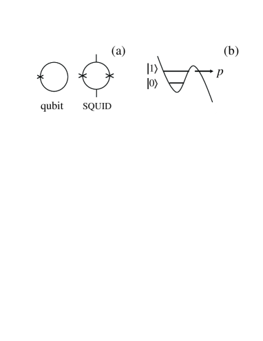
Figure 2: (a) Schematic of a superconducting phase qubit coupled to a SQUID. (b) Energy profile of the qubit with two lowest energy levels in the well representing logic states $|0\rangle$ and $|1\rangle$. Measurement is performed by lowering the energy barrier, so that the state $|1\rangle$ can tunnel out of the well with probability $p$; the tunneling event is then sensed by the SQUID.

By varying the amplitude and duration of the measurement pulse which lowers the barrier, it is possible to control the probability $p$ of tunneling from the level $|1\rangle$, which characterizes the measurement strength. [For a rectangular pulse $p=1-e^{-\Gamma t}$, where $\Gamma$ is the tunneling rate and $t$ is the pulse duration.] Neglecting all imperfections (including finite tunneling from the state $|0\rangle$), the fidelities of such measurement are

$$F_{0}=1,\qquad F_{1}=p.$$ (42)

In the case of measurement result 1 (registered tunneling event) the qubit state is completely destroyed (no longer in the quantum well). However, for measurement result 0 (null-result, no tunneling) the system remains in the quantum well, and therefore it is meaningful to discuss the qubit state evolution due to measurement. Ideally, this evolution should be given by Eq. (1), and this is exactly what has been confirmed in the experiment Katz with good accuracy.

Since the qubit state is destroyed for the measurement result 1, the quantum efficiency $\eta$ cannot be defined, as well as the efficiencies $\tilde{\eta}$, $\tilde{\tilde{\eta}}$, and $\eta_{1}$. However, the null-result efficiency $\eta_{0}$ is a well-defined quantity. In the ideal case described by Eq. (1) the measurement does not dephase the qubit state, and therefore

$$\eta_{0}=1.$$ (43)

In a realistic case there are always some mechanisms, which lead to the qubit decoherence via processes of virtual tunneling, and correspondingly decrease $\eta_{0}$. Some of these processes have been considered theoretically in Ref. Pryadko, , and the results of that paper for the null-result qubit decoherence can be converted into the results for the efficiency $\eta_{0}$.

To estimate experimental quantum efficiency $\eta_{0}$, we use Fig. 3(c) of Ref. Katz, (notice that $\tilde{\eta}_{0}=\eta_{0}$ because $F_{0}=1$). Choosing the data for the initial state $(|0\rangle+|1\rangle)/\sqrt{2}$ and moderate measurement strength ($p\simeq 0.5$), we see that the process of measurement reduces the visibility of the tomography oscillations by less than 7% (we exclude the effects of energy relaxation and dephasing, which occur even in the absence of measurement). Since the theoretical visibility is $[1-4\rho_{00}^{(0)}\rho_{11}^{(0)}(1-e^{-2D_{0}})]^{1/2}$, and since $\rho_{00}^{(0)}\rho_{11}^{(0)}=2/9$ for our initial state and $p=0.5$, we estimate dephasing as $D_{0}\lesssim 0.08$. Using $D_{\min}=-(1/2)\ln(1-p)=\ln 2/2$, we finally convert $D_{0}$ into the quantum efficiency $\eta_{0}\gtrsim 0.8$. Notice that this result most likely underestimates $\eta_{0}$; if we use the decoherence value of 4% obtained in Ref. Katz, in a different way, then the quantum efficiency $\eta_{0}$ is over 90%.

Notice that in the experiment of Ref. Katz, the detection of the tunneling event by SQUID was done after the tomography pulse sequence, and therefore did not affect the quantum efficiency of the partial measurement. If the detection by SQUID should be included into the partial measurement protocol, then it is important to avoid the qubit decoherence by the SQUID operation. This decoherence can be significantly decreased by using the SQUID in the null-result mode also. If the SQUID exceeds its critical current earlier for the tunneled qubit than for the non-tunneled qubit, and if the SQUID is biased in between these two critical currents, then detection of the tunneling event is still accurate; however, in absence of the qubit tunneling the SQUID remains in the “quiet” S-state.

Now let us briefly discuss the natural generalizationPryadko of the null-result measurement of the phase qubit to the case when there is a non-zero probability $p_{0}$ of the qubit tunneling from the state $|0\rangle$. In this case the measurement fidelities are

$$F_{0}=1-p_{0},\qquad F_{1}=p.$$ (44)

Assuming that the coupling between the two qubit states due to tunneling is negligible, we can still use Eq. (1) to describe the null-result evolution.Pryadko In this case the detector is still ideal in the sense that $\eta_{0}=1$ (while $\eta_{1}$, $\eta$, $\tilde{\eta}$, and $\tilde{\tilde{\eta}}$ are still not defined). Notice that for non-zero dephasing $D_{0}$ the definition (26) for $\eta_{0}$ differs from the definition (27) for $\tilde{\eta}_{0}$, in contrast to the above case of $p_{0}=0$, when the two definitions coincide.

IV.4 Tunneling-into-continuum detector

An obvious drawback of the detector considered in the previous subsection is the fact that the qubit state is completely destroyed when the measurement result is 1. In this subsection we consider a detector, which is still based on tunneling into continuum; however, it does not destroy the qubit state for both measurement results. The schematic of the detector is shown in Fig. 3. The initial state of the detector is in the quantum well, and it can tunnel through a barrier into continuum (the phase space is arbitrary). The barrier height is modulated by the qubit state, so that the states $|0\rangle$ and $|1\rangle$ correspond to different rates of tunneling: $\Gamma_{0}$ and $\Gamma_{1}$ (we assume $\Gamma_{1}>\Gamma_{0}$). The measurement is performed during a finite time $t$, after which it is checked if the tunneling has occurred (result 1) or not (result 0). The measurement fidelities are obviously

$$F_{0}=\exp(-\Gamma_{0}t),\qquad F_{1}=1-\exp(-\Gamma_{1}t),$$ (45)

and the goal of this subsection is to analyze the quantum efficiencies of such detector.

The main difference of this detector compared to the detector discussed in the previous subsection is that the tunneling happens in a physical system different from the qubit, and therefore the qubit state is not destroyed by the measurement. As a price for this improvement, the detector now requires two stages: a “sensor” which can tunnel, and then detection of the tunneling event, while for the previous detector the tunneling sensor was physically combined with the qubit. Notice that the model we consider has some similarity with the bifurcation detectors, Siddiqi-05 ; Lupascu-07 ; Dykman-80 which are used for the measurement of qubits (though there are significant differences as wellDykman-07 ).

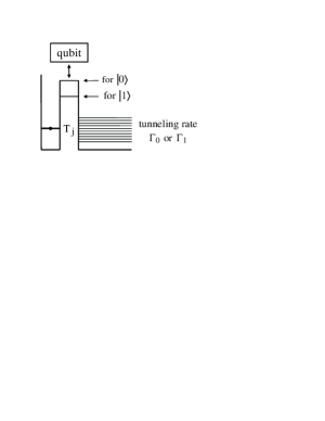
Figure 3: Schematic of a detector based on tunneling into continuum. The qubit state controls the tunneling matrix element ($T_{0}$ or $T_{1}$) and therefore the tunneling rate ($\Gamma_{0}$ or $\Gamma_{1}$).

We describe the qubit-detector system by the following Hamiltonian:

$$H=\sum_{k}\varepsilon_{k}|k\rangle\langle k|+|0\rangle\langle 0|\sum_{k}(T_{0,k}|k\rangle\langle w|+T_{0,k}^{*}|w\rangle\langle k|)$$

$$\hskip 19.91684pt+|1\rangle\langle 1|\sum_{k}(T_{1,k}|k\rangle\langle w|+T_{1,k}^{*}|w\rangle\langle k|),$$ (46)

where the detector Hilbert space consists of the state $|w\rangle$ in the well (its energy is taken to be zero) and many energy levels $|k\rangle$ (with energies $\varepsilon_{k}$) representing the continuum. Since we assume the QND measurement, the qubit Hamiltonian is zero (if energies of states $|0\rangle$ and $|1\rangle$ are actually different, the qubit Hamiltonian is still zero in the rotating frame). The coupling with the qubit changes the detector tunneling matrix elements from $T_{0,k}$ for the qubit state $|0\rangle$ to $T_{1,k}$ for the qubit state $|1\rangle$.

Assuming that the qubit is in one of the logic states $|j\rangle$ ($j=0,1$), the evolution of the detector wavefunction $a_{j}(t)|w\rangle+\sum_{k}b_{j,k}(t)|k\rangle$ is given by equations

$$\dot{a}_{j}=-\frac{i}{\hbar}\sum_{k}T_{j,k}^{*}b_{j,k},\quad\dot{b}_{j,k}=-\frac{i}{\hbar}\varepsilon_{k}-\frac{i}{\hbar}T_{j,k}a_{j}$$ (47)

with the initial condition $a_{j}(0)=1$, $b_{j,k}(0)=0$. Assuming the simplest case when $T_{j,k}=\mbox{const}=T_{j}$ and the energy levels are very dense with constant density of states ${\cal D}$ and infinite energy bandwidth, we obtain the standard solution (see Ref. Pryadko, for better approximations)

$$a_{j}(t)=e^{-\Gamma_{j}t/2},\quad b_{j,k}(t)=\frac{-i}{\hbar}\,T_{j}\,\frac{e^{-\Gamma_{j}t/2}-e^{-i\varepsilon_{k}t/\hbar}}{-\Gamma_{j}/2+i\varepsilon_{k}/\hbar},$$ (48)

where $\Gamma_{j}=(2\pi/\hbar)|T_{j}|^{2}{\cal D}$.

If the initial state of the qubit is $\alpha|0\rangle+\beta|1\rangle$ (where $|\alpha|^{2}+|\beta|^{2}=1$), the evolution is given by superposition of the two evolutions:

$$(\alpha|0\rangle a_{0}+\beta|1\rangle a_{1})|w\rangle+{\small\sum}_{k}(\alpha|0\rangle b_{0,k}+\beta|1\rangle b_{1,k})|k\rangle.$$ (49)

When after time $t$ it is checked if the tunneling event has occured or not, the corresponding probabilities of the measurement outcomes can be obtained by squaring the coefficients in Eq. (49):

$$P_{0}=|\alpha|^{2}e^{-\Gamma_{0}t}+|\beta|^{2}e^{-\Gamma_{1}t},\quad P_{1}=1-P_{0}.$$ (50)

These formulas are obviously consistent with the general description (3) and fidelities (45).

In the case of the measurement result 0 (no tunneling), the state (49) gets projected onto the subspace, which contains only the vector $|w\rangle$ from the detector degrees of freedom; therefore the overall evolution due to measurement is

$$(\alpha|0\rangle+\beta|1\rangle)\,|w\rangle\rightarrow\frac{\alpha|0\rangle\,e^{-\Gamma_{0}t/2}+\beta|1\rangle\,e^{-\Gamma_{1}t/2}}{\sqrt{|\alpha|^{2}e^{-\Gamma_{0}t}+|\beta|^{2}e^{-\Gamma_{1}t}}}\,|w\rangle,$$ (51)

where the denominator is due to normalization and is obviously equal to $\sqrt{P_{0}}$, as in the general description (1). Notice that in Eq. (51) the qubit state is not entangled with the detector [even though it was entangled in the process – see Eq. (49)], and therefore we can say that the qubit state remained pure and underwent a coherent non-unitary evolution described by Eq. (51) without $|w\rangle$. Then considering an arbitrary initial state $\rho$ of the qubit as a mixture of pure states, it is easy to find that the after-measurement state is

$$\rho^{(0)}=\frac{1}{P_{0}}\left(\begin{array}[]{cc}e^{-\Gamma_{0}t}\rho_{00}&e^{-(\Gamma_{0}+\Gamma_{1})t/2}\rho_{01}\\ e^{-(\Gamma_{0}+\Gamma_{1})t/2}\rho_{10}&e^{-\Gamma_{1}t}\rho_{11}\end{array}\right),$$ (52)

where $P_{0}=\rho_{00}e^{-\Gamma_{0}t}+\rho_{11}e^{-\Gamma_{1}t}$. The corresponding quantum efficiency is obviously ideal:

$$\eta_{0}=1,$$ (53)

since $D_{0}=0$.

In the case of the measurement result 1 (tunneling event) the wavefunction (49) is projected onto the subspace orthogonal to $|w\rangle$ and becomes

$$\frac{1}{\sqrt{P_{1}}}\sum_{k}\left(\alpha|0\rangle\frac{-i}{\hbar}\,T_{0}\,\frac{e^{-\Gamma_{0}t/2}-e^{-i\varepsilon_{k}t/\hbar}}{-\Gamma_{0}/2+i\varepsilon_{k}/\hbar}\right.$$

$$\hskip 14.22636pt\left.+\beta|1\rangle\frac{-i}{\hbar}\,T_{1}\,\frac{e^{-\Gamma_{1}t/2}-e^{-i\varepsilon_{k}t/\hbar}}{-\Gamma_{1}/2+i\varepsilon_{k}/\hbar}\right)|k\rangle,\qquad$$ (54)

where the factor $1/\sqrt{P_{1}}$ is again due to normalization. If we want to discuss only the qubit evolution, we have to convert this state into a density matrix and then trace over the detector states $|k\rangle$. It is easy to find that the diagonal matrix elements of thus obtained qubit density matrix $\rho^{(1)}$ are $\rho_{00}^{(1)}=|\alpha|^{2}\sum_{k}|b_{0,k}|^{2}/P_{1}=|\alpha|^{2}(1-e^{-\Gamma_{0}t})/P_{1}$ and $\rho_{11}^{(1)}=|\beta|^{2}\sum_{k}|b_{1,k}|^{2}/P_{1}=|\beta|^{2}(1-e^{-\Gamma_{1}t})/P_{1}$. They are obviously the same as in the general equation (7), since they should obey the classical Bayes formula. To find the off-diagonal matrix element $\rho_{01}^{(1)}=\alpha\beta^{*}\sum_{k}b_{0,k}b_{1,k}^{*}/P_{1}$, we perform integration over the energy $\varepsilon$ using the residue theorem and obtain

$$\rho_{01}^{(1)}=\frac{\alpha\beta^{*}}{P_{1}}\,\frac{4\pi T_{0}T_{1}^{*}\,{\cal D}}{\hbar\,(\Gamma_{0}+\Gamma_{1})}\,[1-e^{-(\Gamma_{0}+\Gamma_{1})t/2}].$$ (55)

Finally, expressing $|T_{0}|$ and $|T_{1}|$ via $\Gamma_{0}$ and $\Gamma_{1}$, and considering arbitrary initial qubit state $\rho$, we find the post-measurement qubit state as

$$\rho^{(1)}=\frac{1}{P_{1}}\left(\begin{array}[]{cc}(1-e^{-\Gamma_{0}t})\rho_{00}&\frac{2\sqrt{\Gamma_{0}\Gamma_{1}}}{\Gamma_{0}+\Gamma_{1}}e^{i\phi_{1}}(1-e^{-\frac{\Gamma_{0}+\Gamma_{1}}{2}t})\rho_{01}\\ \mbox{c.c.}&(1-e^{-\Gamma_{1}t})\rho_{11}\end{array}\right)$$ (56)

where $P_{1}=\rho_{00}(1-e^{-\Gamma_{0}t})+\rho_{11}(1-e^{-\Gamma_{1}t})$ and $\phi_{1}=\arg(T_{0}/T_{1})$. Comparing this result with Eq. (14), we find non-zero decoherence

$$D_{1}=-\ln\left[\frac{2\sqrt{\Gamma_{0}\Gamma_{1}}}{\Gamma_{0}+\Gamma_{1}}\,\frac{1-e^{-(\Gamma_{0}+\Gamma_{1})t/2}}{\sqrt{(1-e^{-\Gamma_{0}t})(1-e^{-\Gamma_{1}t})}}\right].$$ (57)

Since the averaged informational decoherence bound (22) is

$$D_{\min}=-\ln\left[\sqrt{e^{-\Gamma_{0}t}e^{-\Gamma_{1}t}}+\sqrt{(1-e^{-\Gamma_{0}t})(1-e^{-\Gamma_{1}t})}\right],$$ (58)

the quantum efficiency $\eta_{1}$ defined by Eq. (26) is

$$\eta_{1}=\left[1+\frac{\ln\left[\frac{2\sqrt{\Gamma_{0}\Gamma_{1}}}{\Gamma_{0}+\Gamma_{1}}\,\frac{1-e^{-(\Gamma_{0}+\Gamma_{1})t/2}}{\sqrt{(1-e^{-\Gamma_{0}t})(1-e^{-\Gamma_{1}t})}}\right]}{\ln[\sqrt{e^{-(\Gamma_{0}+\Gamma_{1})t}}+\sqrt{(1-e^{-\Gamma_{0}t})(1-e^{-\Gamma_{1}t})}]}\right]^{-1}.$$ (59)

Thick lines in Fig. 4(a) show the dependence of the decoherence $D_{1}$ on the fidelity $F_{1}$ for several ratios of the tunneling rates $\Gamma_{1}/\Gamma_{0}$. [The corresponding values of $1-F_{0}$ are shown by gray lines in Fig. 4(b).] The quantum efficiencies $\eta_{1}$ are shown by thick lines in Fig. 4(b) for the same parameters, and $D_{\min}$ are shown by thin lines in Fig. 4(a). One can see that $D_{1}$ approaches zero and $\eta_{1}$ approaches 100% when $F_{1}\rightarrow 0$ (correspondingly $F_{0}\rightarrow 1$). This behavior can be understood from the result for $b_{j,k}(t)$ given by Eq. (48). It is easy to check that in the case $\Gamma_{1}t\ll 1$ (then $\Gamma_{0}t\ll 1$ also) this result reduces to $b_{j,k}=(-T_{j}/\varepsilon_{k})(1-e^{-i\varepsilon_{k}t/\hbar})$. Since in this case the shape of $b_{j,k}$ dependence on $\epsilon_{k}$ does not depend on $T_{j}$, the qubit state in Eq. (54) becomes disentangled from the detector state, and as a result, the qubit state remains pure. In contrast, when $\Gamma_{1}t\gtrsim 1$, the difference between the shapes of $b_{0,k}$ and $b_{1,k}$ contains an information about the qubit state, which is lost since we do not measure $b_{k}$; as a result, there is a non-zero decoherence of the qubit state. Increase of this lost information with $\Gamma_{1}t$ explains increase of $D_{1}$ and decrease of $\eta_{1}$ with $F_{1}$ in Figs. 4(a) and 4(b). In the limiting case $F_{1}\rightarrow 1$ when $\Gamma_{1}t>\Gamma_{0}t\gg 1$, the decoherence saturates: $D_{1}\rightarrow-\ln[2\sqrt{\Gamma_{0}\Gamma_{1}}/(\Gamma_{0}+\Gamma_{1})]$, while $D_{\min}$ (which describes the information) continues to decrease: $D_{\min}\approx e^{-\Gamma_{0}t}/2$. Since our definition of $\eta_{1}$ is based on comparing $D_{1}$ with $D_{\min}$, this leads to $\eta_{1}\rightarrow 0$, as seen in Fig. 4(b). It is interesting to notice that while the decoherence $D_{1}$ increases with the increase of the ratio $\Gamma_{1}/\Gamma_{0}$ for a fixed $F_{1}$, the efficiency $\eta_{1}$ also increases (instead of decreasing); this is because $D_{\min}$ increases with $\Gamma_{1}/\Gamma_{0}$ faster than $D_{1}$.

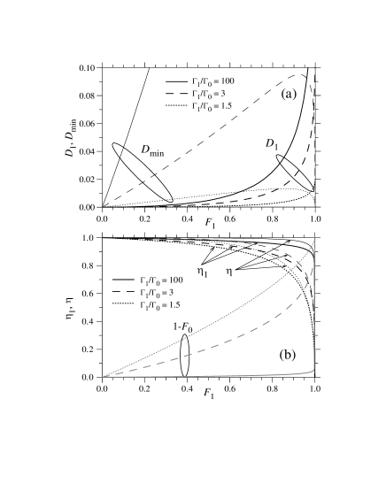
Figure 4: (a) The decoherences $D_{1}$ (thick lines) and $D_{\min}$ (thin lines) and (b) the quantum efficiencies $\eta_{1}$ (thick lines) and $\eta$ (thin lines), as functions of the fidelity $F_{1}$ for a tunneling-into-continuum detector with several values of the ratio of tunneling rates: $\Gamma_{1}/\Gamma_{0}=100$ (solid lines), 3 (dashed lines), and 1.5 (dotted lines). The values of $1-F_{0}$ are shown by gray lines in (b). For the calculation of $\eta$ we have assumed $\phi_{1}=0$. For null-result outcome the detector is ideal: $D_{0}=0$, $\eta_{0}=1$.

For the alternative definition (27) the outcome-dependent quantum efficiencies are

$$\tilde{\eta}_{0}=1,\quad\tilde{\eta}_{1}=\frac{\ln\sqrt{(1-e^{-\Gamma_{0}t})(1-e^{-\Gamma_{1}t})}}{\ln\left[\frac{2\sqrt{\Gamma_{0}\Gamma_{1}}}{\Gamma_{0}+\Gamma_{1}}\,[1-e^{-(\Gamma_{0}+\Gamma_{1})t/2}]\right]}.$$ (60)

If the resulting qubit state is averaged over the measurement results 0 and 1, then the averaged density matrix $\rho^{({\rm av})}=P_{0}\rho^{(0)}+P_{1}\rho^{(1)}$ is

$$\rho^{({\rm av})}=\left(\begin{array}[]{cc}\rho_{00}&e^{-D_{\rm av}}e^{i\phi_{\rm av}}\rho_{01}\\ \mbox{c.c.}&\rho_{11}\end{array}\right),\qquad\qquad$$ (63)

$$e^{-D_{\rm av}}e^{i\phi_{\rm av}}=e^{-\frac{\Gamma_{0}+\Gamma_{1}}{2}t}+\frac{2\sqrt{\Gamma_{0}\Gamma_{1}}}{\Gamma_{0}+\Gamma_{1}}e^{i\phi_{1}}(1-e^{-\frac{\Gamma_{0}+\Gamma_{1}}{2}t}).\,\,\,\,$$ (64)

The quantum efficiencies $\eta$, $\tilde{\eta}$, and $\tilde{\tilde{\eta}}$ can then be calculated using Eqs. (23)–(25) (notice that in our model $\phi_{0}=0$). In particular, when $\phi_{1}=0$ (the qubit does not change the phase of tunneling coefficients) these three efficiencies coincide and are equal to

$$\eta=\frac{\ln\left[e^{-\frac{\Gamma_{0}+\Gamma_{1}}{2}t}+\sqrt{(1-e^{-\Gamma_{0}t})(1-e^{-\Gamma_{1}t})}\right]}{\ln\left[e^{-\frac{\Gamma_{0}+\Gamma_{1}}{2}t}+\frac{2\sqrt{\Gamma_{0}\Gamma_{1}}}{\Gamma_{0}+\Gamma_{1}}(1-e^{-\frac{\Gamma_{0}+\Gamma_{1}}{2}t})\right]}$$ (65)

(the efficiency $\tilde{\eta}$ is given by this expression even if $\phi_{1}\neq 0$). Thin lines in Fig. 4(b) show the quantum efficiency $\eta$ given by Eq. (65) for the same parameters as for $\eta_{1}$. One can see that $\eta>\eta_{1}$; this is because $\eta_{0}=1$ and for our definitions (24) and (26) the value of $\tilde{\eta}$ is always in between $\eta_{0}$ and $\eta_{1}$.

As follows from Eqs. (57), (58), and (65), in the limiting case when there is no tunneling if the qubit is in the state $|0\rangle$ ($\Gamma_{0}\rightarrow 0$, $\Gamma_{1}/\Gamma_{0}\rightarrow\infty$), the results are

$$\eta=1,\,D_{\min}=\frac{\Gamma_{1}t}{2},\,D_{1}=-\ln[\frac{2}{\sqrt{\Gamma_{1}t}}\,\frac{1-e^{-\Gamma_{1}t/2}}{\sqrt{1-e^{-\Gamma_{1}t}}}],$$ (66)

so despite $\eta_{1}\neq 1$, the detector is ideal in the sense $\eta=1$. This happens because in this case for the measurement result 1 the qubit is fully collapsed onto the state $|1\rangle$, so the factor $\sqrt{(1-F_{0})F_{1}}$ in Eq. (14) is zero, and additional dephasing due to $D_{1}$ does not matter. Notice that in this case $\tilde{\eta}_{1}=1$, that illustrates the usefulness of the definition (27).

The main finding of this subsection is that the tunneling-into-continuum detector is ideal for the result 0 (i.e. $\eta_{0}=1$); but it is in general non-ideal for the measurement result 1 ($\eta_{1}<1$), leading to non-ideal averaged efficiency ($\eta<1$). However, the numerical results in Fig. 4(b) show that the quantum efficiencies $\eta_{1}$ and $\eta$ are typically rather close to 100%. [The efficiency $\tilde{\eta}_{1}$ (not shown) is significantly closer to 1 than $\eta_{1}$ and is even higher than $\eta$ for not too large ratio $\Gamma_{1}/\Gamma_{0}$.]

V Conclusion

In this paper we have discussed possible ways to introduce the notion of quantum efficiency for binary-outcome detectors of solid-state qubits. We consider detectors with imperfect measurement fidelities (non-projective measurement) and define the quantum efficiency by comparing the qubit dephasing with the information-related non-unitary evolution dictated by the quantum mechanics.

Our attempt to introduce the quantum efficiency for an arbitrary binary-outcome detector has failed, because the efficiency should in general be characterized by 18 parameters, that is obviously impractical. (The number 18 is the difference between 28 parameters necessary to describe a general binary-outcome detector and 10 parameters necessary to describe an ideal detector, which does not decohere the qubit for each measurement result.)

However, the situation is much simpler for a QND detector. Its operation can be fully characterized by only 6 parameters (instead of 28): fidelity $F_{i}$, phase shift $\phi_{i}$, and decoherence $D_{i}$ for each measurement result ($i=0,1$) – see Eqs. (8)–(15). Therefore it is not difficult to introduce a meaningful definition for the quantum efficiency via a combination of these 6 parameters. However, it can be done in a variety of ways. By comparing the averaged qubit decoherence with the informational bound (22), we have introduced three slightly different definitions: $\eta$, $\tilde{\eta}$, and $\tilde{\tilde{\eta}}$ [see Eqs. (23)–(25)], which are counterparts of the definitionsKor-01 ; Kor-rev of the quantum efficiency for a linear detector. We have also introduced outcome-dependent quantum efficiencies $\eta_{i}$ [see Eq. (26)] by comparing the decoherences $D_{i}$ with the informational bound (22). [Another meaningful way to introduce the outcome-dependent efficiencies is via Eq. (27).] Notice that all these definitions are not applicable in the “orthodox” case of perfect measurement fidelity: $F_{0}=F_{1}=1$.

After introducing the definitions for the quantum efficiency, we have calculated the efficiencies for several simple models of a binary-outcome detector. As follows from the results, it is not easy to find a model for a practical binary-outcome detector which would have theoretically perfect quantum efficiency (in contrast to linear detectors, for which QPC realizes the perfect case). Out of the models we have considered, the perfect efficiency is realized only in the indirect projective measurement, when the qubit interacts with another fully coherent two-level system, which is actually measured. While the quantum efficiency for such measurement setup is ideal, it is not a quite practical setup.

Analyzing a linear detector in the binary-outcome regime (when measurement result is compared with a threshold), we have found that such detector cannot have perfect quantum efficiency: $\eta\leq 2/\pi$, $\eta_{0,1}<0.7$. The tunneling-based partial measurement of superconducting phase qubits is theoretically ideal for the null-result outcome: $\eta_{0}=1$; however, the qubit state is destroyed in the case of the measurement result 1, and therefore quantum efficiencies $\eta_{1}$ and $\eta$ cannot be defined. We have also considered a detector based on tunneling into continuum, which tunneling rate depends on the qubit state. For such a detector the null-result efficiency is also perfect: $\eta_{0}=1$, and even though the efficiencies $\eta_{1}$ and $\eta$ are not perfect, their values can be rather close to 100%.

Our results hint that the practical binary-outcome detectors of solid-state qubits available at present (e.g. bifurcation detectorsVion ; Siddiqi-04 ; Siddiqi-05 ; Lupascu-07 or the balanced comparatorWalls-07 ) cannot closely approach 100% quantum efficiency for both measurement results, even theoretically. However, this is not a rigorous conclusion, and a more detailed analysis of the quantum efficiencies of the particular practical detectors is surely interesting and important.

This work was supported by NSA and IARPA under ARO grant W911NF-04-1-0204.

References

- (1) C. H. Bennett and D. P. DiVincenzo, Nature 404, 247 (2000).
- (2) M. A. Nielsen and I. L. Chuang, Quantum computation and quantum information (Cambridge University Press, Cambridge, 2000).
- (3) J. von Neumann, Mathematical Foundations of Quantum Mechanics (Princeton Univ. Press, Princeton, 1955).
- (4) N. Katz, M. Ansmann, R. C. Bialczak, E. Lucero, R. McDermott, M. Neeley, M. Steffen, E. M. Weig, A. N. Cleland, J. M. Martinis, and A. N. Korotkov , Science 312, 1498 (2006).
- (5) H. M. Wiseman and G. J. Milburn, Phys. Rev. Lett. 70, 548 (1993).
- (6) JM Geremia, J. K. Stockton, and H. Mabuchi, Science 304, 270 (2004).
- (7) R. Ruskov and A. N. Korotkov, Phys. Rev. B 66, 041401(R) (2002).
- (8) A. N. Korotkov and A. N. Jordan, Phys. Rev. Lett. 97, 166805 (2006).
- (9) N. Katz, M. Neeley, M. Ansmann, R. C. Bialczak, M. Hofheinz, E. Lucero, A. O’Connell, H. Wang, A. N. Cleland, J. M. Martinis, and A. N. Korotkov, quant-ph/0806.3547.
- (10) A. N. Korotkov, Phys. Rev. B 60, 5737 (1999).
- (11) A. N. Korotkov, Phys. Rev. B 63, 115403 (2001).
- (12) D. V. Averin, in Quantum noise in mesoscopic physics, edited by Yu. Nazarov (Kluwer, Dordrecht, 2003), p. 229; cond-mat/0301524.
- (13) M. H. Devoret and R. J. Schoelkopf, Nature 406, 1039 (2000).
- (14) Y. Makhlin, G. Schon, and A. Schnirman, Rev. Mod. Phys. 73, 357 (2001).
- (15) S. Pilgram and M. Büttiker, Phys. Rev. Lett. 89, 200401 (2002).
- (16) A. A. Clerk, S. M. Girvin, and A. D. Stone, Phys. Rev. B 67, 165324 (2003).
- (17) A. N. Korotkov, Phys. Rev. B 67, 235408 (2003).
- (18) D. V. Averin and E. V. Sukhorukov, Phys. Rev. Lett. 95, 126803 (2005).
- (19) A. N. Jordan and M. Büttiker, Phys. Rev. B 71, 125333 (2005).
- (20) A. A. Clerk, Phys. Rev. Lett. 96, 056801 (2006).
- (21) A. Shnirman and G. Schön, Phys. Rev. B 57, 15400 (1998).
- (22) A. N. Korotkov, in Quantum noise in mesoscopic physics, edited by Yu. Nazarov (Kluwer, Dordrecht, 2003), p. 205; cond-mat/0209629.
- (23) R. H. Koch, D. J. Van Harlingen, and J. Clarke, Appl. Phys. Lett. 39, 365 (1981).
- (24) C. M. Caves, Phys. Rev. D 26, 1817 (1982).
- (25) V. V. Danilov, K. K. Likharev, and A. B. Zorin, IEEE Trans. Magn. 19, 572 (1983).
- (26) V. B. Braginsky and F. Ya. Khalili, Quantum Measurement (Cambridge Univ. Press, 1992).
- (27) L. Stodolsky, Phys. Lett. B 459, 193 (1999).
- (28) A. N. Korotkov and D. V. Averin, Phys. Rev. B 64, 165310 (2001).
- (29) H.-S. Goan and G. J. Milburn, Phys. Rev. B 64, 235307 (2001).
- (30) T. C. Ralph, S. D. Bartlett, J. L. O’Brien, G. J. Pryde, and H. M. Wiseman, Phys. Rev. A 73, 012113 (2006).
- (31) K. B. Cooper, M. Steffen, R. McDermott, R. W. Simmonds, S. Oh, D. A. Hite, D. P. Pappas, and J. M. Martinis, Phys. Rev. Lett. 93, 180401 (2004).
- (32) J. Claudon, F. Balestro, F. W. J. Hekking, and O. Buisson, Phys. Rev. Lett. 93, 187003 (2004).
- (33) D. Vion, A. Aassime, A. Cottet, P. Joyez, H. Pothier, C. Urbina, D. Esteve, and M. H. Devoret, Science 296, 886 (2002).
- (34) I. Siddiqi, R. Vijay, F. Pierre, C. M. Wilson, M. Metcalfe, C. Rigetti, L. Frunzio, and M. H. Devoret, Phys. Rev. Lett. 93, 207002 (2004)
- (35) I. Siddiqi, R. Vijay, F. Pierre, C. M. Wilson, L. Frunzio, M. Metcalfe, C. Rigetti, R. J. Schoelkopf, M. H. Devoret, D. Vion, and D. Esteve, Phys. Rev. Lett. 94, 027005 (2005).
- (36) A. Lupascu, S. Saito, T. Picot, P. C. De Groot, C. J. P. M. Harmans, and J. E. Mooij, Nature Phys. 3, 119 (2007).
- (37) L. P. Pryadko and A. N. Korotkov, Phys. Rev. B 76, 100503(R) (2007).
- (38) M. I. Dykman and M. A. Krivoglaz, Physica A 104, 480 (1980).
- (39) M. I. Dykman, Phys. Rev. E 75, 011101 (2007).
- (40) T. J. Walls, D. V. Averin, and K. K. Likharev, IEEE Trans. Appl. Supercond. 17, 136 (2007).