Revisit of interfacial free energy of the hard sphere system near hard wall

Abstract

We propose a simple Monte Carlo method to calculate the interfacial free energy $\gamma$ between the substrate and the material. Using this method we investigate the interfacial free energys of the hard sphere fluid and solid phases near a smooth hard wall. According to the obtained interfacial free energys of the coexisting fluid and solid phases and the Young equation we are able to determine the contact angle with high accuracy, $\cos\theta=1.010(31)$, which indicates that a smooth hard wall can be wetted completely by the hard sphere crystal at the interface between the wall and the hard sphere fluid.

I Introduction

The interfacial free energy(IFE) $\gamma$ between different materials or different phases of a material plays crucial roles in many physical phenomena such as wetting and spreading de Gennes . An accurate result for $\gamma$ is necessary to understand these phenomena completely. The hard sphere system as a simple model system of condensed matter has been investigated extensively. By changing the density of the system, it undergoes a first order phase transformation from the liquid phase to the FCC solid phase Hoover . An interesting problem of the hard sphere system related to the IFE is whether a smooth hard wall can be wetted completely by the hard sphere crystal in the density region of coexistence. The problem was studied by different groups in the past but a definite answer is still awaiting Courtemanche ; Courtemanche1 ; Kegel . Recent computer simulation Dijkstra by Dijkstra provided a strong evidence of complete wetting. In that paper the author investigated the effect of wall separation on crystalline layers at the walls in a double-wall system and extracted the complete wetting information from the phenomenon of surface freezing(including complete wetting and capillary freezing). Alternatively, the direct way to study this wetting behavior is to calculate the cosine of the contact angle in terms of Young equation, i.e. $\cos\theta=(\gamma_{fw}^{c}-\gamma_{sw}^{c})/\gamma_{fs}^{c}$, here the subscripts $f$, $s$ and $w$ denote respectively the fluid, solid and wall, and the superscript $c$ denotes the bulk coexisting phase. In the complete wetting state $\cos\theta$ given by the above formula will be larger than unity. The fluid-wall IFE $\gamma_{fw}$ can be estimated via density functional theory Ohnesorge ; Gotzelmann , scaled particle theory Reiss , molecular dynamic simulation Henderson and Monte Carlo(MC) simulation Heni ; Gloor ; MacDowell . However, it is unfeasible to calculate directly the solid-wall IFE $\gamma_{sw}$ using the above methods except for the MC simulation Heni . Recently, several groups have calculated the crystal/melt IFE $\gamma_{fs}^{c}$ of a hard sphere system by different computer simulation methods Davidchack ; Cacciuto ; Davidchack1 ; Mu ; Davidchack2 . However, the accuracies of the contact angle $\theta$ from their calculation are too low to conclude definitely whether or not the wetting is complete Dijkstra . Comparing with $\gamma_{fs}^{c}$, the error of the contact angle $\theta$ comes mainly from $\gamma_{fw}^{c}$ and $\gamma_{sw}^{c}$ Heni ; Davidchack2 . Therefore, it is desired to accurately calculate the IFEs, which provide us not only the confirming of the complete wetting scenario but also a benchmark to test other theoretical methods.

In this paper we propose a simple Monte Carlo method of calculating the IFEs $\gamma_{fw}$ and $\gamma_{sw}$, and obtain the IFEs of the coexisting hard sphere fluid and solid phase(i.e. $\gamma_{fw}^{c}$ and $\gamma_{sw}^{c}$) with high accuracy, which nearly confirms the suggestion that at the smooth hard wall-hard sphere fluid interface a complete wetting phase transition occurs very close to the bulk freezing transition. Our method is inspired by the cleaving method of Davidchack and Laird Davidchack , where they used two moving walls to transform the hard sphere system from the bulk phase into the phase confined completely by two walls and vice versa, and the IFE can be obtained by calculating the work done in the reversible process. However, as mentioned in Davidchack’s work Davidchack , irreversibility is introduced during cleaving a fluid system using constructed hard walls. The reason of irreversibility is that the system doesn’t reach the equilibrium state in a typical run, which can be reduced by increasing the duration of equilibration run. The problem can be avoided by designing an auxiliary path which connects the confined and the bulk phase and the states along the path are all in equilibrium state during the simulation. The goal is achieved by combine the cleaving technique Davidchack ; Broughton and the so-called flat histogram methods Berg ; Wang ; Wang1 . From these method $\gamma_{fw}$ and $\gamma_{sw}$ can be accurately estimated. In the following sections we employ Wang-Landau (WL) algorithm Wang to demonstrate the implementation of the current approach.

In order to check the validity of our method, we calculated the IFE between the hard sphere system and the smooth hard wall at usual densities, including $\gamma_{fw}$ and $\gamma_{sw}$ for three different crystal orientations $(1,1,1)$, $(1,1,0)$, and $(1,0,0)$. The results are consistent with those of Heni and Löwen within the statistical error Heni . We also investigated the finite size effect of longitudinal dimension(along $z$ direction) on the IFE, and then obtained the effective interaction potential between two hard walls. Finally, we use the method to calculate the IFEs of the coexisting phase $\gamma_{fw}^{c}$ and $\gamma_{sw}^{c}$, and then obtained the contact angle $\cos\theta$. The paper is organized as follows: in section II, the model system and the numerical algorithm are described. The results are presented in section III. Section IV is a brief conclusion.

II Model and Algorithm

Our system is composed of $N$ hard sphere particles with diameter $\sigma$ in a fixed volume $V$. The periodic boundary conditions are imposed in all three directions. Hard sphere system is athermal, therefore its thermodynamic properties are solely dependent on the dimensionless packing fraction $\eta=\pi\rho\sigma^{3}/6$, where $\rho$ is the number density of the particles. Pairs of particles $i$ and $j$ interact via the potential

$$U_{Hs}(\vec{r_{i}},\vec{r_{j}})=\left\{\begin{array}[]{ll}\infty,&{\rm when}\quad|\vec{r_{i}}-\vec{r_{j}}|<\sigma,\\ 0,&{\rm otherwise},\end{array}\right.$$ (1)

here $\vec{r}$ is the positions of the particles.

Figure 1: Diagram illustrating the change of the system boundary conditions by two synchronously moving smooth hard walls. When the walls are respectively placed on $|a_{1}|$ and $|a_{2}|$ ($|a_{1}|=|a_{2}-Z_{0}|=D_{0}>\sigma/2$), they do not interact with the particles and the system is in the bulk phase; when the walls are placed at the boundaries, the system are completely confined by two hard walls.

Two moving smooth hard walls are used to transform the system from the periodic boundary conditions into the hard wall boundary conditions, as Davidchack and Laird did Davidchack . The detail is illustrated in Figure 1. The two walls can be displaced synchronously along $z$ direction from the boundary of the system (shown by the dot line in Figure 1) to the position $a_{1}$ and $a_{2}$ ($|a_{1}|=|a_{2}-Z_{0}|>\sigma/2$, $Z_{0}$ is the dimension of the system in the $z$-direction), respectively. The interaction between the walls and the particles is

$$U_{w}(\vec{z_{i}},\vec{z_{w}})=\left\{\begin{array}[]{ll}\infty,&{\rm when}\quad|\vec{z_{i}}-\vec{z_{w}}|<\sigma/2,\\ 0,&{\rm otherwise},\end{array},\right.$$ (2)

where $\vec{z_{i}}$ and $\vec{z_{w}}$ are the coordinates of the particles and the walls in $z$ direction, respectively. Therefore, when the separation between the walls and the boundaries is larger than the hard sphere radius, the walls do not interact with the particles and the system is in the bulk phase; however, when the walls are placed at the boundaries, the system are completely confined by the two hard walls.

The total Hamiltonian of the system $H$ is a sum of the kinetic energy and the potential energy, given by

$$K=\sum_{i}\frac{P_{i}^{2}}{2m}$$ (3)

and

$$U=\sum_{i<j}U_{Hs}(\vec{r_{i}},\vec{r_{j}})+U_{w}(\vec{z_{i}},\vec{z}_{w1},\vec{z}_{w2}),$$ (4)

where $m$ is the mass of particles and $p_{i}$ is the linear momenta. The Helmholtz free energy of the system is written as

$$F(T,V,N,z_{w1},z_{w2})=-k_{B}T\;{\rm ln}(Q(T,V,N,z_{w1},z_{w2})),$$ (5)

where $Q(T,V,N,z_{w1},z_{w2})$ is the canonical partition function of the system

$$Q(T,V,N,z_{w1},z_{w2})=\frac{1}{\Lambda^{3N}N!}\int dr_{1}^{3}\cdots\int dr_{N}^{3}\exp(-\beta U(\{\vec{r}_{i}\},z_{w1},z_{w2})).$$ (6)

In the leading order approximation, the total IFE is just the difference of the total free energy between the confined system and the bulk system Evans ; Heni . The IFE per unit area $\gamma$ is expressed by

$$\gamma(\eta,T) = \frac{F_{confined}(T,\eta)-F_{bulk}(T,\eta)}{A}$$ (7)

$$= \frac{F(T,\eta,z_{w1}=0,z_{w2}=Z_{0})-F(T,\eta,z_{w1}=a1,z_{w2}=a2)}{A},$$

here $A$ is the total contact area between the system and two hard walls.

Using WL algorithm Wang , initially developed to compute the density of state(DOS) $g(E)$, we can easily obtain the excess Helmholtz free energy in a Metropolis-type MC simulation. The original algorithm does a random walk in energy space with an acceptance ratio $\min\{1,g(E_{i})/g(E_{f})\}$, where $E_{i}$ and $E_{f}$ are respectively the energies of the current and the proposed configuration. The DOS of the accepted energy then adjusted by multiply it with a factor $f>1$. The histogram is accumulated in the simulation and its flatness is tested. A new run with reduced $f$ starts when the histogram reaches a specified flatness condition. The DOS obtained when the $f$ reduced close to unity.

The same procedure can be used to calculated the excess Helmholtz free energy. In order to use the method, we employ an expanded canonical ensemble, where the separation $D_{wb}$ from the hard walls to the system boundary is an additional ensemble variable. The expanded ensemble method has been used to calculate the Helmholtz free energy at a series of temperatures Lyubartsev and the chemical potential of polymers Wilding and colloid Tej . Obviously, $0\leq D_{wb}\leq D_{0}$, where $D_{0}=|a_{1}|=|a_{2}-Z_{0}|$. We use $D_{wb}$ to rewrite (7) as

$$\gamma(\eta,T)=\frac{F(T,\eta,D_{wb}=0)-F(T,\eta,D_{wb}=D_{0})}{A}.$$ (8)

Every $D_{wb}$ corresponds to a macroscopic state. The DOS $g(D_{wb})$ of the system can be computed via WL algorithm. For the hard interaction system, the logarithm of DOS is proportional to the partition function of the system. According to (5) and (8) we get

$$\gamma(\eta,T)=\frac{k_{B}T\ln(g(D_{wb}=D_{0}))-k_{B}T\ln(g(D_{wb}=0))}{A}.$$ (9)

The expanded canonical ensemble simulations are performed in a similar way as in the canonical ensemble. In addition to the particles translation operation which is accepted or rejected in the usual way, the trial moves also include the walls displacement along $z$ axis, which is accepted with the probability

$$P_{acc}\{D_{wb}^{old}\rightarrow D_{wb}^{new}\}=\min\{1,g(D_{wb}^{old})/g(D_{wb}^{new})\},$$ (10)

Where $D_{wb}^{old}$ and $D_{wb}^{new}$ are the distances before and after the hard walls are displaced, respectively. In other words a random walk is implemented in $D_{wb}$ space instead of energy space. The calculation is as follows, the interval $[0,D_{0}]$ is divided into many subintervals, a random walk in this space is performed in the same way as that of the Wang-Landau method in the energy space. A initial guess of the DOS is assigned, the walk goes on with the acceptance probability given by (9) and a initial factor $f>1$, the DOS of the accepted state is modified by multiply the corresponding DOS with $f$. A histogram of accepted states is accumulated and the flatness of it is tested. The run is finished when the histogram is flat enough, here we use the criteria that the deviation of the histogram away from its average is less than 20%. A new run starts with the DOS obtained in the previous run as initial DOS and the factor $f$ is reduced to $\sqrt{f}$. The full calculation is ended when the reduce factor $f$ is very close to $1$, here we use $f-1<10^{-5}-10^{-6}$. At the end of the simulation the $\gamma(\eta,T)$ can be determined from equation (9).

III Results and Discussion

The simulations were performed in a cuboid box with conventional periodic boundary conditions. The $D_{wb}$ is a continuous variable, however the WL algorithm demands a discrete $D_{wb}$. In the calculation the continuous $D_{wb}$ is replaced with a set of discrete points and the walls may displace by jumping between nearest-neighbor points. Increasing $D_{wb}$ and decreasing $D_{wb}$ are attempted with equal frequency, which are accepted or rejected by transition rule (10). At first, we check the validity of our method by calculating $\gamma_{fw}$ and $\gamma_{sw}$ at two ordinary densities.

III.1 Fluid-wall $\gamma$

In this subsection we report the results of the $\gamma$ for the fluid-wall interface. The transverse dimensions of the simulation box are respectively $L_{x}=8.1\sigma$ and $L_{y}=7\sigma$. In order to study the longitudinal finite size effect we consider several different longitudinal dimensions $L_{z}=6.6\sigma$, $L_{z}=13.2\sigma$, $L_{z}=19.8\sigma$, $L_{z}=26.4\sigma$ and $L_{z}=33.1\sigma$, and the number of particles $N$ are respectively $216$, $432$, $648$, $864$ and $1080$, which correspond to a packing fraction of $\eta=0.3$. The dependence of $\gamma_{fw}^{*}=\gamma_{fw}\sigma^{2}$ on $L_{z}$ is shown in Figure 2. The $\gamma_{fw}^{*}$ decreases with increasing the longitudinal dimension of the system at fixed packing fraction and the curve flattens gradually. In other words, there exists an effective interaction potential $\Phi_{\rm eff}$ between the two walls, which is a function of $L_{z}$ and can be written as

$$\Phi_{\rm eff}(L_{z})=A(\gamma_{fw}(L_{z})-\gamma_{fw}(\infty)),$$ (11)

here $A$ is the total contact area and $\gamma_{fw}(\infty)$ is the exact IFE.

Our result of the $\gamma_{fw}^{*}$ at the largest separation, $L_{z}=33.1$, is $0.652\pm 0.005)kT/\sigma^{2}$, which can be regarded as a good approximation of the exact IFE and this value is in very good agreement with that of Heni’s Heni , $\gamma_{fw}^{*}=(0.656\pm 0.03)kT$. We also performed simulations for a system with $L^{{}^{\prime}}_{x}\times L^{{}^{\prime}}_{y}\simeq 2(L_{x}\times L_{y})$ and $L^{{}^{\prime}}_{z}=33.1\sigma$, the results are basically the same as that of the results obtained from the smaller system which indicates our system size is already big enough.

Figure 2: Data points (with error bars) show the reduced fluid-wall interfacial free energy $\gamma_{fw}^{*}$ at $\eta=0.3$. The solid line is merely a guide to the eye.

III.2 Solid-wall $\gamma$

In the solid-wall case the initial configuration is an ideal fcc lattice with periodic boundary conditions. The system dimensions $L_{x}$, $L_{y}$, and $L_{z}$ are given in Table 1 and the number of particles $N$ are determined in such a way that the volume fraction remains constant, $\eta=0.6$. Here, we calculate the crystal-wall $\gamma_{sw}$ for the three crystalline orientations $(1,1,1)$, $(1,1,0)$ and $(1,0,0)$. The results are compared with those of Heni’s in Table 1. The resulting $\gamma_{sw}^{*}$ as a function of $L_{z}$ are plotted in Figure 3. The profiles of the IFE and the effective potential are similar to those of the fluid phase. However, the IFEs are largely anisotropic and their ratio is $\gamma_{110}:\gamma_{100}:\gamma_{111}\approx 5:3:2$ at $\eta=0.6$, which implies a hard sphere solid prefers to pack in the $(1,1,1)$ orientation near a smooth hard wall. We also checked the lateral finite size effects of the crystal-wall $\gamma_{sw}$ for three orientations, all results are consistent with those obtained from the smaller systems within statistical error.

	$L_{x}$	$L_{y}$	$L_{z1}$	$L_{z2}$	$L_{z3}$	$L_{z4}$	$L_{z5}$	$\gamma^{*}$	$\gamma^{*}_{1}$
111	6.4$\sigma$	5.6$\sigma$	5.3$\sigma$	10.6$\sigma$	21$\sigma$	26.3$\sigma$		2.09$\pm$0.01	1.74$\pm$0.21
100	6.1$\sigma$	6.1$\sigma$	12.1$\sigma$	18.2$\sigma$	24.1$\sigma$	30.3$\sigma$		3.02$\pm$0.01	2.95$\pm$0.30
110	6.1$\sigma$	8.6$\sigma$	15$\sigma$	18.2$\sigma$	21.4$\sigma$	24.7$\sigma$	30$\sigma$	5.08$\pm$0.01	5.03$\pm$0.30

Table 1: The system dimensions and interfacial free energys with their statistical error for three crystal face orientations. $\gamma^{*}$: our simulation result; $\gamma^{*}_{1}$: MC simulation form Ref. [11].

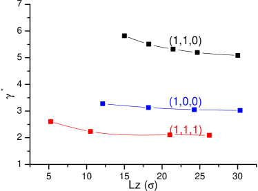
Figure 3: Data points show the crystal-wall reduced interfacial free energy $\gamma_{sw}^{*}$ for three different orientations at $\eta=0.6$. From bottom to top: (1,1,1), (1,0,0) and (1,1,0) orientation. The solid line is merely a guide to the eye. Statistical errors do not exceed the symbol size.

III.3 Wetting

The IFEs of the coexisting phases $\gamma_{fw}^{c}$ and $\gamma_{sw}^{c}$ are calculated in this section. Based on the results of the last subsections, we expect that the simulation systems with lateral dimensions $L_{x}\times L_{y}\simeq 60\sigma^{2}$ and longitudinal dimension $L_{z}\simeq 38\sigma$ is large enough to effectively reduce the finite-size effect. It is worth emphasizing that the coexisting volume fractions of the hard sphere fluid and solid phases are $\eta_{f}=0.4917$ and $\eta_{s}=0.543$ Davidchack ; Mu ; Davidchack2 ; Davidchack3 , respectively, which are slightly different from those obtained by Hoover and Ree Hoover . Because the hard sphere particles usually crystalize on a smooth hard wall with the $(1,1,1)$ orientation, we need only consider this packing structure. The $\gamma_{sw}^{c}$ can be easily determined, however, the prefreezing phenomenon prevents us from directly achieving the $\gamma_{fw}^{c}$ from the simulation. We have to extrapolate the $\gamma_{fw}$ from lower packing fraction to the bulk coexisting packing fraction $\eta_{f}$ Heni . In order to get a more accurate estimation of the $\gamma_{fw}$ at the bulk coexisting packing fraction, we should use the data at packing fractions as close to the bulk coexisting as possible, on the other hand, the data used should correspond to fluid phases, i.e., before the prefreezing occurs. Therefore, it’s crucial to accurately locate the volume fraction just before the prefreezing. Our simulation results are the relative Helmholtz free energy of the system with various $D_{wb}$, therefore, if the prefreezing occurs so that crystalline layers appear at some $D_{wb}$ value, a singularity may be observed on the free energy versus $D_{wb}$ curve. Figure 4 depicts the free energy-$D_{wb}$ curve for different packing fractions $\eta$ close to the bulk coexisting packing. The volume fractions of the system from top to bottom are respectively $\eta_{f}$, $0.9975\eta_{f}$, $0.995\eta_{f}$, $0.9925\eta_{f}$ and $0.99\eta_{f}$. From Figure 4 we see that the packing fraction of forming the crystalline layers is lower than $0.995\eta_{f}$, however it is difficult to locate the point exactly. With these observations it is appropriate to extrapolate from the volume fraction $\eta=0.99\eta_{f}$. On the other hand, by observing the density profile near the walls Dijkstra Dijkstra suggested that at the packing fraction $\eta\sim 0.987\eta_{f}$ the crystalline layers begin to form. To check the consistence of the extrapolation, we also obtained the IFE by extrapolations from $\gamma_{fw}$ at the volume fraction $\eta=0.985\eta_{f}=0.4843$. The two extrapolation results are the same within statistical error of the simulation. The results of the IFE are shown in Table 2. In Figure 5 we compare our simulation results with those from the scaled particle theory combined with the Carnahan-Starling equation of state(SPT) Heni . Here we don’t present a comparison with Heni’s simulation results, as the coexistence densities taken in their simulation are different from ours.

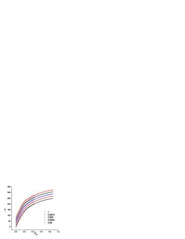
Figure 4: (color online)The relative Helmholtz free energy versus the parameter $D_{wb}$ for different packing fractions. From top to bottom the packing fraction $\eta=\eta_{f}$, $0.9975\eta_{f}$, $0.995\eta_{f}$, $0.9925\eta_{f}$ and $0.99\eta_{f}$. The shape of the upper curves obviously differs from the lower curves, which indicates the formation of the crystalline layers. The curves are shifted vertically for clarity.

  $\eta$ $\gamma^{*}$ $\delta$ 0.20 0.3261 0.0004 0.25 0.4685 0.0004 0.30 0.6499 0.0004 0.35 0.8836 0.0011 0.40 1.1866 0.0007 0.43 1.4106 0.0010 0.46 1.6711 0.0011 0.4843 1.9105 0.0016 0.4867 1.9323 0.0018 0.4917_f 1.9872 0.0012 0.4917${}_{f_{1}}$ 1.9896 0.0016 0.5430_s 1.4380 0.0050  

Table 2: The reduced surface free energys $\gamma^{*}$ with its error $\delta$ for different volume fractions. The subscript $f$ and $f_{1}$ refer to the surface tension of coexisting hard sphere fluid phase $\gamma_{fw}^{c*}$ obtained by extrapolating from $0.99\eta_{f}$ and $0.985\eta_{f}$, respectively. And the subscript $s$ refers to the surface free energy of coexisting hard sphere solid phase $\gamma_{sw}^{c*}$ with $(1,1,1)$ face.

Using the available latest crystal/melt IFE $\gamma_{fs}=0.546(16)$ from simulation Davidchack2 combined with our results, the contact angle $\theta$ can be calculated in terms of the Young equation, $\cos\theta=(\gamma_{fw}^{c}-\gamma_{sw}^{c})/\gamma_{fs}^{c}=1.010(31)$, which nearly indicates that a complete wetting phase transition will occur. If the above $\gamma_{fs}^{c}$ is replaced by the value $0.55(2)$ obtained from nucleation experiment Marr , which is the average of the crystal/melt IFEs over all three orientations and larger than the $\gamma_{fs}^{c}$ for (1,1,1) interface, we will have the same conclusion. The main source of error is the crystal/melt IFE $\gamma_{fs}^{c}$, a more accurate $\gamma_{fs}^{c}$ is necessary to draw a definite conclusion. Of course, one can also improve the precision of the $\gamma_{fw}^{c}$ and $\gamma_{sw}^{c}$ by employing other sampling method, e.g. multicanonical algrithm Berg .

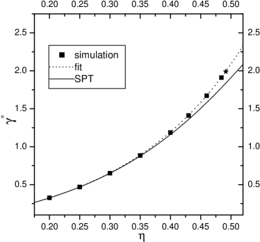
Figure 5: The fluid-wall reduced surface tension versus the volume fraction. The solid line denotes SPT; the dashed line denotes a numerical fit from SPT; the filled square refers to our simulation results and $\star$ to the $\gamma_{fw}^{c*}$ obtained from extrapolation.

IV conclusion

In conclusion, we proposed a simple Monte Carlo method and calculated the IFEs of the hard sphere system at the smooth hard wall with high accuracy. The contact angle calculated with the accurate IFEs $\gamma_{fw}^{c}$ and $\gamma_{sw}^{c}$ make us confident that a smooth hard wall can be completely wetted by the hard sphere crystal at the wall-hard sphere fluid interface. Our conclusion is consistent with Dijkstra’s work. However, when using the Young equation to study the wetting behavior, the finite-size effect can not be avoided completely as Dijkstra did in Ref. [6]. Therefore larger system and higher precision are necessary to confirm unambiguously the complete wetting phenomenon. Furthermore, the IFEs obtained also provide a benchmark to test other theoretical approaches. Our method can be extended to other systems (e.g. soft sphere system, polydisperse hard sphere system and hard/soft wall system) in a straightforward manner. We have already obtained some results of the polydisperse hard sphere system which will be reported elsewhere.

Note added in proof. — After the completion of this study, we are aware of Laird et al studied the same problem with molecular dynamics simulation and have the same conclusions as ours Laird . The work is supported by the National Natural Science Foundation of China under grant No.10334020 and in part by the National Minister of Education Program for Changjiang Scholars and Innovative Research Team in University.

References

- (1) P. G. de Gennes, Rev. Mod. Phys., 1985, 57, 827.
- (2) W. G. Hoover and F. H. Ree, J. Chem. Phys., 1968, 49, 3609.
- (3) D. J. Courtemanche and F. van Swol, Phys. Rev. Lett., 1992, 69, 2078.
- (4) D. J. Courtemanche, T. A. Pasmore, and F. van Swol, Mol. Phys., 1993, 80, 861.
- (5) W. K. Kegel, J. Chem. Phys., 2001, 115, 6538.
- (6) M. Dijkstra, Phys. Rev. Lett., 2004, 93, 108303.
- (7) R. Ohnesorge, H. Löwen, and H. Wagner, Phys. Rev. E, 1994, 50, 4801.
- (8) B. Gotzelmann, A. Haase, and S. Dietrich, Phys. Rev. E, 1996, 53, 3456.
- (9) H. Reiss, H. L. Frisch, E. Helfand, and J. L. Lebowitz, J. Chem. Phys., 1960, 32, 119.
- (10) J. R. Henderson and F. van Swol, Mol. Phys., 1984, 51, 991.
- (11) M. Heni and H. Löwen, Phys. Rev. E., 1999, 60, 7057.
- (12) G. J. Gloor, G. Jackson, F. J. Blas and E. de Miguel, J. Chem. Phys., 2005, 123, 134703.
- (13) L. G. MacDowell and P. Bryk, Phys. Rev. E, 2007, 75, 061609.
- (14) R. L. Davidchack and B. B. Laird, Phys. Rev. Lett., 2000, 85, 4751.
- (15) A. Cacciuto, S. Auer, and D. Frenkel, J. Chem. Phys., 2003, 119, 7467 .
- (16) R. L. Davidchack and B. B. Laird, Phys. Rev. Lett., 2005, 94, 086102.
- (17) Y. Mu, A. Houk, and X. Song, J. Phys. Chem. B, 2005, 109, 6500.
- (18) R. L. Davidchack, J. R. Morris, and B. B. Laird, J. Chem. Phys., 2006, 2125, 094710.
- (19) J. Q. Broughton and G. H. Gilmer, J. Chem. Phys., 1986, 84, 5759.
- (20) B. A. Berg and T. Neuhaus, Phys. Rev. Lett., 1992, 68, 9.
- (21) F. Wang, D. P. Landau, Phys. Rev. Lett., 2001, 86, 2050.
- (22) J. S. Wang and R. H. Swendsen, J. Stat. Phys., 2002, 106, 245.
- (23) R. Evans in Liquids at Interfaces, Les Houches Session XLVIII, edited by J. Charvolin, J. F. Joanny, and J. Zinn-Justin (Elsevier, Amsterdam, 1990)
- (24) A. P. Lyubartsev, A. A. Martsinovski, S. V. Shevkunov, and P. N. Vorontsov-Velyaminov, J. Chem. Phys., 1992, 96, 1776.
- (25) N. B. Wilding and M. Muller, J. Chem. Phys., 1994, 101, 4324.
- (26) M. K. Tej and J. C. Meredith, J. Chem. Phys., 2002, 117, 5443.
- (27) R. L. Davidchack and B. B. Laird, J. Chem. Phys., 1998, 108, 9452.
- (28) D.W. Marr and A. P. Gast, Langmuir, 1994, 10, 1348.
- (29) B. B. Laird and R. L. Davidchack, J. Phys. Chem. C, 2007, 111, 15952 .