Detailed Study of the $K_{L}\to\pi^{0}\pi^{0}\pi^{0}$ Dalitz Plot

Abstract

Using a sample of $68.3$ million $K_{L}\to\pi^{0}\pi^{0}\pi^{0}$ decays collected in 1996-1999 by the KTeV  (E832) experiment at Fermilab, we present a detailed study of the $K_{L}\to\pi^{0}\pi^{0}\pi^{0}$ Dalitz plot density. We report the first observation of interference from $K_{L}\to\pi^{+}\pi^{-}\pi^{0}$ decays in which $\pi^{+}\pi^{-}$ rescatters to $\pi^{0}\pi^{0}$ in a final-state interaction. This rescattering effect is described by the Cabibbo-Isidori model, and it depends on the difference in pion scattering lengths between the isospin $I=0$ and $I=2$ states, $a_{0}-a_{2}$. Using the Cabibbo-Isidori model, and fixing $(a_{0}-a_{2})m_{\pi^{+}}=0.268\pm 0.017$ as measured by the CERN-NA48 collaboration, we present the first measurement of the $K_{L}\to\pi^{0}\pi^{0}\pi^{0}$ quadratic slope parameter that accounts for the rescattering effect: $h_{000}=(+0.59\pm 0.20_{stat}\pm 0.48_{syst}\pm 1.06_{ext})\times 10^{-3}$, where the uncertainties are from data statistics, KTeV  systematic errors, and external systematic errors. Fitting for both $h_{000}$ and $a_{0}-a_{2}$, we find ${h}_{000}=(-2.09\pm 0.62_{stat}\pm 0.72_{syst}\pm 0.28_{ext})\times 10^{-3}$, and $m_{\pi^{+}}({a}_{0}-{a}_{2})=0.215\pm 0.014_{stat}\pm 0.025_{syst}\pm 0.006_{ext}$ ; our value for $a_{0}-a_{2}$ is consistent with that from NA48.

I Introduction

The amplitude for the $K_{L}\to\pi^{0}\pi^{0}\pi^{0}$ decay includes contributions from two sources. The first source is from intrinsic dynamics that represent a $K_{L}$ decaying directly into the $\pi^{0}\pi^{0}\pi^{0}$ final state. The second contribution is from the decay $K_{L}\to\pi^{+}\pi^{-}\pi^{0}$ followed by a rescattering, $\pi^{+}\pi^{-}\to\pi^{0}\pi^{0}$. The amplitudes from these two contributions result in a small $(\sim 1\%)$ interference pattern in the Dalitz plot density.

The Dalitz plot density corresponding to the intrinsic $K\to 3\pi$ decay amplitude is approximately described by Particle Data Group (2006)

$$|{\cal M}^{int}(X_{D},Y_{D})|^{2}\propto 1+gY_{D}+\sqrt{3}jX_{D}+hY_{D}^{2}+3kX_{D}^{2}~{},$$ (1)

where

$$X_{D} \equiv (s_{1}-s_{2})/(\sqrt{3}m_{\pi^{+}}^{2})$$ (2)

$$Y_{D} \equiv (s_{3}-s_{0})/m_{\pi^{+}}^{2}$$ (3)

$$s_{i} \equiv (P_{K}-P_{i})^{2},~{}~{}i=1,2,3$$ (4)

$$s_{0} \equiv (s_{1}+s_{2}+s_{3})/3~{},$$ (5)

and $P_{K}$ and $P_{i}$ are the four-momenta of the parent kaon and the three pions. The linear $g,j$ parameters and the quadratic $h,k$ parameters are determined experimentally. For the specific case of $K_{L}\to\pi^{0}\pi^{0}\pi^{0}$ decays, the linear terms vanish, $h=3k$ and the intrinsic Dalitz plot density reduces to Messner et al. (1974); Devlin and Dickey (1979)

$$|{\cal M}_{000}^{\rm int}|^{2}\propto 1+h_{000}R^{2}_{D}~{},$$ (6)

where

$$R^{2}_{D} = X_{D}^{2}+Y_{D}^{2}$$ (7)

$$= \frac{4}{m_{\pi^{+}}^{4}}\left[s_{0}^{2}-(s_{1}s_{2}+s_{1}s_{3}+s_{2}s_{3})/3\right]~{},$$ (8)

and $h_{000}$ is the quadratic slope parameter. With $|h_{000}|<10^{-2}$ and $R^{2}_{D}<2.5$ from kinematic constraints, the variation of $|{\cal M}_{000}|^{2}$ over the entire Dalitz plot is less than 2%.

There are two previous measurements of $h_{000}$. The first reported measurement, from Fermilab experiment E731 Somalwar et al. (1992), is based on 5 million recorded $K_{L}\to\pi^{0}\pi^{0}\pi^{0}$ decays with an $R^{2}_{D}$-resolution $\sigma(R^{2}_{D})\sim 0.1$ determined from Monte Carlo simulations. CERN experiment NA48 Lai et al. (2001) used nearly 15 million decays with $\sigma(R^{2}_{D})\simeq 0.03$. The average of these two results is $h_{000}({\rm PDG06})=(-5.0\pm 1.4)\times 10^{-3}$ Particle Data Group (2006). Here we report a more precise result from KTeV  based on $68.3$ million decays with $\sigma(R^{2}_{D})\simeq 0.014$. Compared with the previous measurements of $h_{000}$, a major difference in the KTeV  analysis is that we take into account the contribution from $K_{L}\to\pi^{+}\pi^{-}\pi^{0}$ decays in which $\pi^{+}\pi^{-}\to\pi^{0}\pi^{0}$ in a final-state interaction.

A full treatment of rescattering in $K\to 3\pi$ decays, including higher order loop corrections, is given by Cabibbo and Isidori Cabibbo and G.Isidori (2005). This model, referred to hereafter as CI3PI, describes a “cusp” in the region where the minimum $\pi^{0}\pi^{0}$ mass is very near $2m_{\pi^{+}}$: a cusp refers to a localized region of the Dalitz plot where the density changes very rapidly. A precisely measured shape of this cusp can be used to measure the difference in pion scattering lengths between the isospin $I=0$ and $I=2$ states, $a_{0}-a_{2}$. In 2006, the CERN-NA48 collaboration reported the first observation of a cusp in $K^{\pm}\to\pi^{\pm}\pi^{0}\pi^{0}$ decays. The interference effect is from the decay $K^{\pm}\to\pi^{\pm}\pi^{\mp}\pi^{\pm}$ followed by rescattering: $\pi^{+}\pi^{-}\to\pi^{0}\pi^{0}$. They reported $(a_{0}-a_{2})m_{\pi^{+}}=0.268\pm 0.017$ Batley et al. (2006), in excellent agreement with the prediction of Chiral Perturbation Theory Colangelo et al. (2000, 2001).

Compared to $K^{\pm}\to\pi^{\pm}\pi^{0}\pi^{0}$ decays, a much smaller cusp is expected in $K_{L}\to\pi^{0}\pi^{0}\pi^{0}$ decays, and here we report the first such observation as part of our measurement of the quadratic slope parameter. The expected distortion of the $K_{L}\to\pi^{0}\pi^{0}\pi^{0}$ Dalitz plot is shown in Fig. 1a using $h_{000}=-0.005$ and no contribution from rescattering, and in Fig. 1b using $h_{000}=0$ and CI3PI Cabibbo and G.Isidori (2005) to model rescattering from $K_{L}\to\pi^{+}\pi^{-}\pi^{0}$.

The effects of rescattering and a negative value of $h_{000}$ both result in the Dalitz plot density dropping slowly as $R^{2}_{D}$ increases. The maximum variation is only a few percent. The main feature that separates these two effects is that while the quadratic slope parameter results in a smooth linear function of $R^{2}_{D}$, the rescattering from $K_{L}\to\pi^{+}\pi^{-}\pi^{0}$ results in a much sharper fall-off near some of the Dalitz plot edges (see “cusp” labels in Fig. 1b). Also note that the Dalitz plot density in Fig. 1a is azimuthally symmetric, while the density in Fig. 1b is azimuthally asymmetric. This cusp will become more apparent when we examine the minimum $\pi^{0}\pi^{0}$ mass in § VI.

The outline of this report is as follows. The KTeV  detector and simulation are described in § II-III. The reconstruction of $K_{L}\to\pi^{0}\pi^{0}\pi^{0}$ decays and the determination of the Dalitz plot variables ($X_{D},Y_{D}$) are presented in § IV. § V describes the fitting technique used to extract the quadratic slope parameter ($h_{000}$) and the difference in scattering lengths ($a_{0}-a_{2}$). Systematic uncertainties are described in § VII, and § VIII presents results for $h_{000}$ with $a_{0}-a_{2}$ fixed to the value measured by the NA48 collaboration. In § IX, both the quadratic slope parameter and the difference in scattering lengths are determined simultaneously in a two-parameter fit of the $K_{L}\to\pi^{0}\pi^{0}\pi^{0}$ phase space.

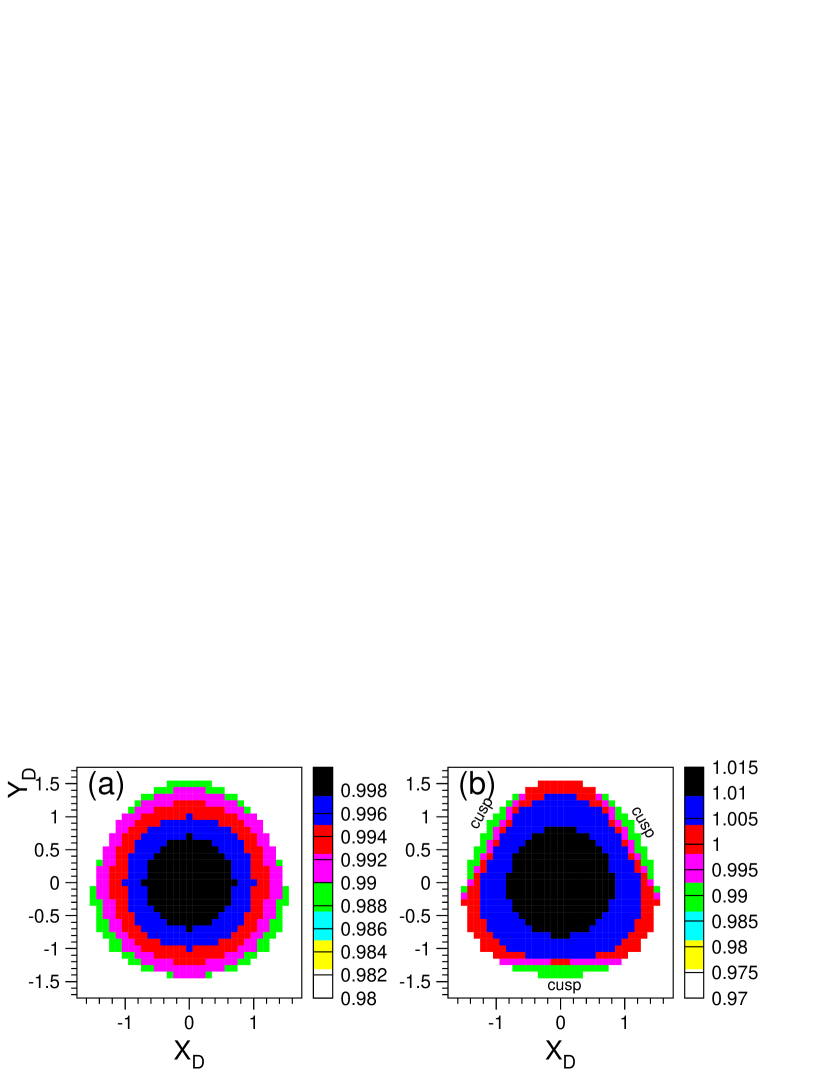
Figure 1: Expected deviation from $K_{L}\to\pi^{0}\pi^{0}\pi^{0}$ phase-space based on (a) $h_{000}=-0.005$ and no contribution from rescattering, and (b) $K_{L}\to\pi^{+}\pi^{-}\pi^{0}$ with rescattering as calculated by Cabibbo and Isidori Cabibbo and G.Isidori (2005), with $h_{000}=0$. The intensity scales are slightly different to better illustrate the relative shapes.

II Experimental Apparatus

The KTeV  detector has been described in detail elsewhere Alavi-Harati et al. (2003); Alexopoulos et al. (2004). Here we give a brief description of the essential detector components. An 800 GeV proton beam incident on a beryllium-oxide (primary) target produces neutral kaons along with other charged and neutral particles. Sweeping magnets remove charged particles from the beamline. Beryllium absorbers 20 meters downstream of the target attenuate the beam in a manner that increases the kaon-to-neutron ratio. A collimation system results in two parallel neutral beams beginning 90 meters from the primary target; each beam consists of roughly equal numbers of kaons and neutrons. The fiducial decay region is 121-158 meters from the target, and the vacuum region extends from 20-159 meters. A regenerator, designed to produce $K_{S}$ decays for the $Re(\epsilon^{\prime}/\epsilon)$ measurement, alternates between the two beams. The other neutral beam is called the vacuum ($K_{L}$) beam. Only $K_{L}\to\pi^{0}\pi^{0}\pi^{0}$ decays from the vacuum beam are used in this analysis.

The KTeV  detector (Fig. 2) is located downstream of the decay region. The main element used in the analysis is an electromagnetic calorimeter made of 3100 pure cesium iodide (CsI) crystals (Fig. 3). For photons and electrons, the energy resolution is better than 1% and the position resolution is about 1 mm. The CsI calorimeter has two holes to allow the neutral beams to pass through without interacting.

A spectrometer consisting of four drift chambers, two upstream and two downstream of a dipole magnet, measures the momentum of charged particles; the resolution is $\sigma_{p}/p\simeq[1.7\oplus(p/14)]\times 10^{-3}$, where $p$ is the track momentum in GeV/$c$. Bags filled with helium are placed between the drift chambers and inside the magnet, replacing about 25 meters of air. A scintillator “trigger” hodoscope just upstream of the CsI is used to trigger on decays with charged particles in the final state. The KTeV  beamline has very little material upstream of the CsI calorimeter, thereby reducing the impact of external photon conversions ($\gamma X\to Xe^{+}e^{-}$). The total amount of material is 0.043 radiation lengths, about half of which is in the trigger hodoscope. Eight photon-veto detectors along the decay region and spectrometer reject events with escaping particles.

An electronic trigger for $K_{L}\to\pi^{0}\pi^{0}\pi^{0}$ decays requires at least 25 GeV total energy deposit in the CsI calorimeter, as well as six isolated clusters with energy above 1 GeV. For $K_{L}\to\pi^{0}\pi^{0}\pi^{0}$ decays that satisfy the energy and vertex requirements (§ IV), approximately 9% of these decays satisfy the six-cluster trigger, and 20% of the six-cluster events were recorded for analysis. The combined six-cluster data from three run periods (1996, 1997, 1999) has nearly 400 million recorded events. $K_{L}\to\pi^{0}\pi^{0}\pi^{0}$ decays are recorded for use as a high-statistics crosscheck on the Monte Carlo (see below) determination of the acceptance in the $Re(\epsilon^{\prime}/\epsilon)$ analysis Alavi-Harati et al. (2003). This sample is ideal to study the Dalitz density.

Figure 2: Plan view of the KTeV  (E832) detector. The evacuated decay volume ends with a thin vacuum window at $Z=159$ m. Only decays from the vacuum beam are used to measure $h_{000}$.

Figure 3: Layout of CsI calorimeter. The two neutral beams go through the $15\times 15~{}{\rm cm}^{2}$ beam holes (into page) shown by the two inner squares. The fiducial cut, indicated by the dark lines, rejects $K_{L}\to\pi^{0}\pi^{0}\pi^{0}$ decays in which any photon hits a crystal adjacent to a beam hole or at the outer boundary.

III Monte Carlo Simulation

A Monte Carlo simulation (MC) is used to determine the expected $K_{L}\to\pi^{0}\pi^{0}\pi^{0}$ Dalitz plot density that would be observed without the contribution from rescattering and with $h_{000}=0$; i.e, pure phase space. The $K_{L}\to\pi^{0}\pi^{0}\pi^{0}$ dynamics are determined from deviations between the observed Dalitz density (Fig. 5) and that from the phase-space MC. The simulated phase-space density accounts for detector geometry, detector response, trigger, and selection requirements in the analysis.

The simulation of $K_{L}\to\pi^{0}\pi^{0}\pi^{0}$ decays begins by selecting the kaon momentum from a distribution measured with $K\to\pi^{+}\pi^{-}$ decays. Each simulated kaon undergoes scattering in the beryllium absorbers near the target, and kaons that hit the edge of any collimator are either scattered or absorbed. For kaons that scatter from a collimator edge, the $K_{L}$-$K_{S}$ mixture has been determined from a study of $K_{L}\to\pi^{+}\pi^{-}\pi^{0}$ and $K^{0}\to\pi^{+}\pi^{-}$ decays. After generating a kaon trajectory downstream of the collimator, each photon from $K_{L}\to\pi^{0}\pi^{0}\pi^{0}\to 6\gamma$ is traced through the detector, allowing for external ($\gamma\to e^{+}e^{-}$) conversions. The secondary electron-positron pairs are traced through the detector and include the effects of multiple scattering, energy loss from ionization, and bremsstrahlung. The effects of accidental activity are included by overlaying events from a trigger that recorded random activity in the detector that is proportional to the instantaneous intensity of the proton beam.

For photons and electrons that hit the CsI calorimeter, the energy response is taken from a shower library generated with geant Brun et al. (1994): each library entry contains the energy deposits in a $13\times 13$ grid of crystals centered on the crystal struck by the incident particle. The shower library is binned in incident energy, position within a crystal, and angle.

For both data and MC, the energy calibration for the CsI is performed with momentum-analyzed electrons from $K_{L}\to\pi^{\pm}e^{\mp}\nu$ decays. To match CsI energy resolutions for data and MC, an additional 0.3% fluctuation is added to the MC energy response. The data also show a low-side response tail that is not present in the MC, and is probably due to photo-nuclear interactions in the CsI calorimeter. As explained in Appendix B of Alexopoulos et al. (2004), this energy-loss tail has been accurately measured with electrons from $K_{L}\to\pi^{\pm}e^{\mp}\nu$ decays, and this tail is empirically modeled in the simulation with the assumption that the energy-loss tail is the same for photons and electrons. Losses up to 40% of the incident photon/electron energy are included in the model.

The CsI position resolution is measured with precise electron trajectories in $K_{L}\to\pi^{\pm}e^{\mp}\nu$ decays. The position resolution for the MC is found to be nearly 10% worse than for data, requiring that the MC cluster positions be “un-smeared” to match the data resolution. The un-smearing is done for each simulated photon cluster by moving the reconstructed position closer to the true (generated) position in the CsI calorimeter. The position un-smearing fraction is $0.07+0.0016E_{\gamma}$, where $E_{\gamma}$ is the photon energy in GeV.

Nearly five billion $K_{L}\to\pi^{0}\pi^{0}\pi^{0}$ decays were generated by our Monte Carlo simulation. More than 90% of the generated decays are rejected by the geometric requirement that all six photons hit the CsI calorimeter; about 2/3 of these six-cluster events are rejected by the selection requirements described below in § IV. The resulting sample of $124.9$ million reconstructed $K_{L}\to\pi^{0}\pi^{0}\pi^{0}$ decays corresponds to $1.8\times$ the data statistics.

IV Reconstruction of $K_{L}\to\pi^{0}\pi^{0}\pi^{0}$ Decays

The reconstruction of $K_{L}\to\pi^{0}\pi^{0}\pi^{0}\to 6\gamma$ is based on measured energies and positions of photons that hit the CsI calorimeter. Exactly six clusters, each with a transverse profile consistent with a photon, are required. The cluster positions must be separated by at least $7.5$ cm, and each cluster energy must be greater than $3$ GeV. For the two nearest photon clusters in the CsI calorimeter, we require that the minimum-to-maximum photon energy ratio is greater than 20%; this requirement eliminates the most extreme cases of overlapping clusters in which an energetic photon lands very close to a photon of much lower energy. The fiducial volume is defined by cluster positions measured in the calorimeter; we reject events in which any reconstructed photon position is in a crystal adjacent to a beam-hole or in the outermost layer of crystals (Fig. 3).

To remove events in which the kaon has scattered in the collimator or regenerator, we define the center-of-energy of the six photon clusters to be

$$x_{ce}=\sum_{i}x_{i}E_{i}/\sum_{i}E_{i}~{}~{}~{}~{}~{}~{}~{}~{}y_{ce}=\sum_{i}y_{i}E_{i}/\sum_{i}E_{i}$$ (9)

where $x_{i},y_{i}$ are the measured photon positions in the CsI calorimeter, $E_{i}$ are the measured photon energies, and the index $i=1,6$. The coordinate $x_{ce},y_{ce}$ is the point where the kaon would have intercepted the plane of the calorimeter if it had not decayed. The size of each beam at the CsI calorimeter is about $10\times 10~{}{\rm cm}^{2}$; the center-of-energy, measured with $\sim 1$ millimeter resolution, is required to lie within an $11\times 11~{}{\rm cm}^{2}$ square centered on the kaon beam.

Photons are paired to reconstruct three neutral pions consistent with a single decay vertex. There are 15 possible photon pairings for a $K_{L}\to\pi^{0}\pi^{0}\pi^{0}$ decay. To select the best $\pi^{0}\pi^{0}\pi^{0}$ pairing, we introduce a “pairing-$\chi^{2}$” variable ($\chi_{pair}^{2}$), which quantifies the consistency of the three $\pi^{0}$ vertices. To ensure a reliable reconstruction of the Dalitz variables, we require that the smallest of the 15 $\chi_{pair}^{2}$ values is less than 10 (the mean $\chi_{pair}^{2}$ is 3), and also that the second smallest $\chi_{pair}^{2}$ value is greater than 30. The location of the kaon decay vertex ($z$) is determined from a weighted average of the $\pi^{0}$ vertices.

The main kinematic requirement is that the invariant mass of the $\pi^{0}\pi^{0}\pi^{0}$ final state be between $0.494$ and $0.501$ GeV/$c^{2}$, or nearly $\pm 4\sigma$. Figure 4a shows the $\pi^{0}\pi^{0}\pi^{0}$-mass distribution for data and the MC. The mass side-bands are due to $K_{L}\to\pi^{0}\pi^{0}\pi^{0}$ decays in which the wrong photon pairing is found in the reconstruction. The fraction of reconstructed events outside the invariant mass cut is $0.21\%$ for data and $0.20\%$ for the MC, confirming that the MC provides an excellent description of the data.

Additional selection requirements are that the energy-sum of the six photon clusters lie between 40 and 160 GeV, and that the reconstructed decay vertex is within 121–158 meters from the primary target. To prevent an accidental cluster from faking a photon, we use the energy-vs-time profiles recorded by the CsI calorimeter. For each photon candidate, the CsI cluster energy deposited in a 19 nanosecond window before the event must be consistent with pedestal. To limit the effect of external photon conversions in the detector material ($\gamma X\to Xe^{+}e^{-}$), we allow no more than one hit in the scintillator hodoscope that lies 2 meters upstream of the CsI calorimeter.

To improve the resolution of the Dalitz plot parameters ($X_{D},Y_{D},R^{2}_{D}$), the cluster energies are adjusted for each event by imposing kinematic constraints to minimize

$$\chi_{E}^{2}=\sum_{i=1}^{6}\frac{(E_{i}-E_{i}^{fit})^{2}}{\sigma_{i}^{2}}~{},$$ (10)

where $E_{i}$ are the reconstructed cluster energies, $\sigma_{i}$ are the energy resolutions, and $E_{i}^{fit}$ are the six fitted cluster energies. The impact of cluster position resolution on the Dalitz parameters is much smaller than that of the energy resolution, and therefore the cluster positions are fixed in the minimization. The four kinematic constraints are $M_{6\gamma}=M_{K}$ and $M_{\gamma\gamma}=m_{\pi^{0}}$ for each of the three neutral pions. With four constraints and six unknowns in Eq. 10, the minimization has two degrees of freedom. Events with $\chi_{E}^{2}<50$ are selected for the analysis. The minimization of $\chi_{E}^{2}$ improves the $R^{2}_{D}$-resolution from 0.070 to $0.014$. Fig. 4b shows a data-MC comparison of the $\chi_{E}^{2}$ distribution. The fraction of events removed by the $\chi_{E}^{2}$ cut is $0.43\%$ for data and $0.47\%$ for the MC; this slight disagreement will be addressed in the evaluation of systematic uncertainties.

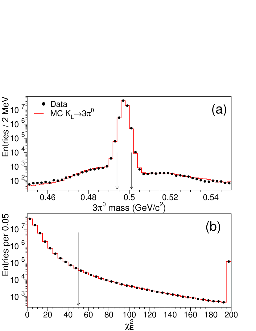
Figure 4: (a) Invariant $\pi^{0}\pi^{0}\pi^{0}$ mass with all selection requirements except for the $\pi^{0}\pi^{0}\pi^{0}$-mass and $\chi_{E}^{2}$. The $\pi^{0}\pi^{0}\pi^{0}$ mass resolution (from Gaussian fit) is $0.94~{}{\rm MeV}/c^{2}$. (b) shows $\chi_{E}^{2}$ distribution with all other selection requirements; last bin includes all events with $\chi_{E}^{2}>200$. Dots are data and the histogram is MC. Vertical arrows show the selection requirements.

After all reconstruction and selection requirements there are $68.3$ million $K_{L}\to\pi^{0}\pi^{0}\pi^{0}$ events. The two-dimensional Dalitz plot distribution for this sample is shown in Fig. 5 with no acceptance correction, and projections onto $R^{2}_{D}$ and the minimum $\pi^{0}\pi^{0}$ mass are shown in Fig. 6a,b. The $\sim 5$% variation across the Dalitz plot is mainly from the detector acceptance; this variation is nearly an order of magnitude larger than the variations from rescattering (CI3PI) and the quadratic slope parameter. Also note that the uncorrected phase space distribution has a minimum at the center of the Dalitz plot, while the expected effects from physics (Fig. 1) result in a maximum at the center. An accurate $K_{L}\to\pi^{0}\pi^{0}\pi^{0}$ simulation is therefore critical to this measurement.

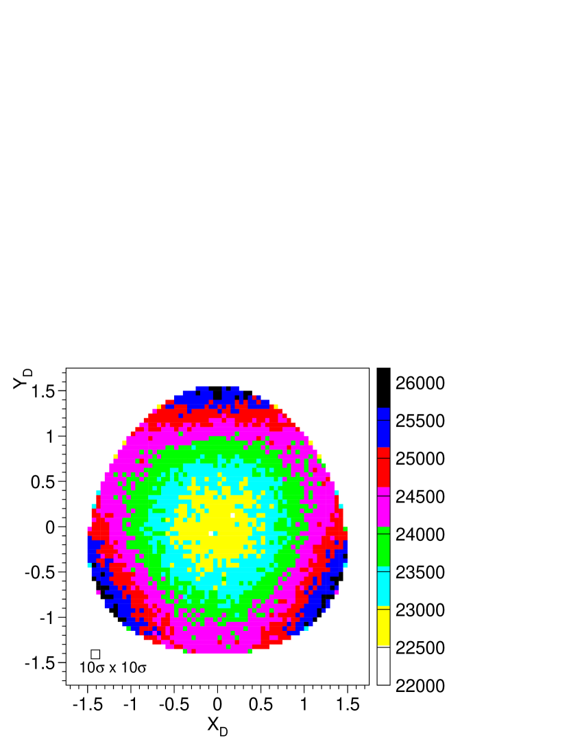
Figure 5: Dalitz plot density, $Y_{D}$ vs. $X_{D}$, for $68.3$ million $K_{L}\to\pi^{0}\pi^{0}\pi^{0}$ decays in the KTeV  data sample after all selection requirements. The color-scale at right shows the number of events in each $0.05\times 0.05$ pixel. The reconstruction resolution on $X_{D}$ and $Y_{D}$ is $\sigma\sim 0.01$ as determined by the MC; the box in the lower-left corner shows $10\sigma\times 10\sigma$ for illustration.

V Fit for $h_{000}$ and $a_{0}-a_{2}$

In the previous measurements of the quadratic slope parameter $h_{000}$ Somalwar et al. (1992); Lai et al. (2001), the $R^{2}_{D}$-distribution for data (Fig. 6a) was compared to the $R^{2}_{D}$ distribution from a simulated $K_{L}\to\pi^{0}\pi^{0}\pi^{0}$ sample with $h_{000}=0$. Normalizing the MC sample to have the same data statistics at $R^{2}_{D}=0$, the data/MC ratio was fit to a linear function, $1+h^{\prime}R^{2}_{D}$, where $h^{\prime}$ is the fitted slope. The region $R^{2}_{D}>1.9$ was excluded because this region is more sensitive to energy nonlinearities and resolution. The $K_{L}\to\pi^{0}\pi^{0}\pi^{0}$ slope parameter was then assumed to be $h_{000}=h^{\prime}$. Applying the same procedure to our KTeV  data yields a result consistent with the CERN-NA48 result Lai et al. (2001), but with a very poor fit probability.

In light of new information about rescattering from $K_{L}\to\pi^{+}\pi^{-}\pi^{0}$, we fit our two-dimensional Dalitz plot to the CI3PI model Cabibbo and G.Isidori (2005). With the exception of $h_{000}$ and $a_{0}-a_{2}$, the CI3PI model parameters have been measured or calculated theoretically, and these parameters are listed in Table 1. In this section the fitting technique is described within the framework of a single-parameter fit for $h_{000}$ with the value of $a_{0}-a_{2}$ fixed by an external measurement (from NA48). However, this fitting technique works the same way when both $h_{000}$ and $a_{0}-a_{2}$ are floated in the fit.

Table 1: Parameters and their values used in the CI3PI model. $K_{3\pi}$ refers to $K_{L}\to\pi^{+}\pi^{-}\pi^{0}$, subscripts 0 and 2 refer to isospin $I=0$ and $I=2$.

parameter	value
$K_{3\pi}$ linear slope ($g_{+-0}$)	$0.678\pm 0.008$ Particle Data Group (2006)
$K_{3\pi}$ quadratic slope ($h_{+-0}$)	$0.076\pm 0.006$ Particle Data Group (2006)
$a_{0}m_{\pi^{+}}$ at $\pi^{+}\pi^{-}$ thresh	$0.216\pm 0.013$ S.Pislak et al. (2003)
$(a_{0}-a_{2})m_{\pi^{+}}$ at $\pi^{+}\pi^{-}$ thresh	$0.268\pm 0.017$ Batley et al. (2006)
Effective ranges ($r_{0},r_{2}$)	$1.25\pm 0.04$, $1.81\pm 0.05$ Cabibbo and G.Isidori (2005)
$A_{L}^{+}/A_{L}^{0}$	$0.28\pm 0.03$ Cabibbo and G.Isidori (2005)
Isospin breaking parameter ($\epsilon$)	0.065 Batley et al. (2006)

We first define $N_{xy}^{\rm data}$ to be the number of events reconstructed in a $0.05\times 0.05$ Dalitz pixel (Fig. 5) denoted by integers $x$ and $y$. The model prediction for the number of events in each Dalitz pixel, $N_{xy}^{\rm pred}$, is given by

$$N_{xy}^{\rm pred}=~{}~{}~{}~{}~{}~{}~{}~{}~{}~{}~{}~{}~{}~{}~{}~{}~{}~{}$$

$${\cal N}\sum_{{}^{x^{\prime}=x-2,x+2}_{y^{\prime}=y-2,y+2}}|{\cal M}_{000}(x^{\prime},y^{\prime})|^{2}N_{x^{\prime}y^{\prime}}^{\rm MC}{\rm PSF}(x^{\prime}-x,y^{\prime}-y)~{}.$$ (11)

The quantities appearing in the prediction function are explained as follows. ${\cal N}$ is an overall normalization factor such that the total phase-space density integrals on each side of Eq. 11 are the same. ${\cal M}_{000}(x^{\prime},y^{\prime})$ is the matrix element at the center of pixel $x^{\prime},y^{\prime}$, as calculated from the CI3PI model and the floated value of $h_{000}$. The remaining quantities are based on $K_{L}\to\pi^{0}\pi^{0}\pi^{0}$ MC generated with $h_{000}=0$ and no rescattering: i.e., flat phase space. $N_{x^{\prime}y^{\prime}}^{\rm MC}$ is the number of $K_{L}\to\pi^{0}\pi^{0}\pi^{0}$ events generated in pixel $x^{\prime},y^{\prime}$ that pass all selection criteria; note that $N_{x^{\prime}y^{\prime}}^{\rm MC}$ is not the number of MC events reconstructed in pixel $x^{\prime},y^{\prime}$. ${\rm PSF}(x^{\prime}-x,y^{\prime}-y)$ is the “pixel-spread-function,” computed from MC, which gives the fraction of events generated in pixel $x^{\prime},y^{\prime}$ that are reconstructed in pixel $x,y$. In each of the 2956 Dalitz pixels with data, the ${\rm PSF}$ is computed on a $5\times 5$ grid around the pixel. The pixel size corresponds to about $5\sigma\times 5\sigma$ in terms of the reconstruction resolution of $X_{D}$ and $Y_{D}$. On average, 70% of the MC events are reconstructed in the same Dalitz pixel as the generation pixel; 99.96% of the MC events are reconstructed within a $3\times 3$ pixel grid centered on the generation pixel.

The data are fit with minuit to minimize the $\chi^{2}$-function

$$\chi^{2}=\sum_{x,y}\left[(N_{xy}^{\rm data}-N_{xy}^{\rm pred})/\sigma_{xy}^{\rm pred}\right]^{2}~{},$$ (12)

where $N_{xy}^{\rm pred}$ is the prediction function in Eq. 11, and $N_{xy}^{\rm data}$ is the number of reconstructed $K_{L}\to\pi^{0}\pi^{0}\pi^{0}$ decays in pixel $x,y$. The statistical uncertainty is

$$(\sigma_{xy}^{\rm pred})^{2}=N_{xy}^{\rm pred}+(N_{xy}^{\rm pred})^{2}/N_{xy}^{\rm MC}$$ (13)

where $N_{xy}^{\rm MC}$ is the number of MC events reconstructed in pixel $x,y$. The two terms above represent the statistical uncertainty on the data and MC, respectively.

In the fitting procedure we make an additional selection requirement that among the three possible $\pi^{0}\pi^{0}$ pairings, the minimum $\pi^{0}\pi^{0}$ mass, “$m_{\pi^{0}\pi^{0}}^{\rm min}$,” is greater than $0.274~{}{\rm GeV}/c^{2}$. This requirement removes 3 million (4.5%) $K_{L}\to\pi^{0}\pi^{0}\pi^{0}$ decays from the data sample, and it is applied because of a slight data-model discrepancy that is discussed in § VII.2 and § VIII.1.

The quality of the fit is illustrated by the $\chi^{2}$. With $h_{000}$ as a fit parameter and $a_{0}-a_{2}$ fixed, $\chi^{2}/{\rm dof}=2805.3/2765$ for all of the pixels, and $\chi^{2}_{\rm edge}/{\rm dof}=125.3/130$ for the subset of edge-pixels that overlap the Dalitz boundary. The sensitivity of $\chi^{2}_{\rm edge}$ is illustrated by fitting the data without the kinematically-constrained energy adjustments (Eq. 10): in this case, $\chi^{2}_{\rm edge}$ increases by 60. Fitting for both $h_{000}$ and $a_{0}-a_{2}$, the corresponding $\chi^{2}$ and $\chi^{2}_{\rm edge}$ are very similar. The results of these fits are presented in § VIII-IX.

Figure 6: For the $68.3$ million $K_{L}\to\pi^{0}\pi^{0}\pi^{0}$ in the KTeV  sample, projected Dalitz distributions are shown for (a) $R^{2}_{D}$ and (b) $m_{\pi^{0}\pi^{0}}^{\rm min}$. The average reconstruction resolution determined by the simulation is $\sigma(R^{2}_{D})\sim 0.014$ and $\sigma({\rm min}~{}m_{\pi^{0}\pi^{0}})\sim 0.3$ MeV$/c^{2}$: these resolutions are indicated by a $10\sigma$ marker on each plot. The data/MC(phase-space) ratio is shown as a function of (c) $R^{2}_{D}$ and (d) $m_{\pi^{0}\pi^{0}}^{\rm min}$ (points with error bars). The solid curve is the prediction from our best fit $h_{000}$. The dashed curve is the prediction using $h_{000}({\rm PDG06})=(-5.0\pm 1.4)\times 10^{-3}$. The arrow in (d) shows the selection requirement $m_{\pi^{0}\pi^{0}}^{\rm min}>0.274~{}{\rm GeV}/c^{2}$. Note that previous analyses Somalwar et al. (1992); Lai et al. (2001) ignored rescattering and excluded $R^{2}_{D}>1.9$ ; the corresponding data/MC ratio was assumed to be a straight line with slope of $-0.005$.

VI Observation of Interference from $K_{L}\to\pi^{+}\pi^{-}\pi^{0}$ with Rescattering

While the cusp from rescattering is clearly visible in the CERN-NA48 distribution of $m_{\pi^{0}\pi^{0}}$ from $K^{\pm}\to\pi^{\pm}\pi^{0}\pi^{0}$ decays (see Fig. 2 of Batley et al. (2006)), there is no such evidence in our raw distribution of $m_{\pi^{0}\pi^{0}}^{\rm min}$ from $K_{L}\to\pi^{0}\pi^{0}\pi^{0}$ decays (Fig. 6b). The rescattering effect in $K_{L}\to\pi^{0}\pi^{0}\pi^{0}$ decays becomes apparent only when the data are divided by the corresponding MC distribution generated with pure phase-space: i.e, $h_{000}=0$ and no rescattering from $K_{L}\to\pi^{+}\pi^{-}\pi^{0}$ decays. These data/MC(phase-space) ratios are shown as data points with errors in Figs. 6c,d. A cusp is clearly visible in the Dalitz region $R^{2}_{D}\sim 2$ and $m_{\pi^{0}\pi^{0}}^{\rm min}\sim 2m_{\pi^{+}}=0.28~{}{\rm GeV}$. The rescattering process $\pi^{+}\pi^{-}\to\pi^{0}\pi^{0}$ changes from a virtual process ($m_{\pi^{+}\pi^{-}}<2m_{\pi^{+}}$) resulting in destructive interference, to a real process ($m_{\pi^{+}\pi^{-}}>2m_{\pi^{+}}$) resulting in constructive interference.

We use the fit results (§ VIII) to compute a prediction for the data/MC(phase-space) ratio as a function of $R^{2}_{D}$ and $m_{\pi^{0}\pi^{0}}^{\rm min}$; these predictions are shown as solid curves in Figs. 6c,d. The predictions agree well with our measured data/MC(phase-space) distributions, except for the discrepancy in the region defined by $m_{\pi^{0}\pi^{0}}^{\rm min}<0.274~{}{\rm GeV}/c^{2}$ (first four bins of Fig. 6d). The dashed curves show the prediction using the CI3PI model and $h_{000}$ replaced with the current PDG value, $h_{000}=-0.005$; these curves clearly do not match the KTeV  distributions. To easily reproduce the KTeV prediction, we have parametrized the solid curve in Fig. 6d as a polynomial of the form:

$${\mathcal{R}}_{00}^{\rm model}(m_{\pi^{0}\pi^{0}}^{\rm min})=\sum_{n=0}^{3}m_{i}\times(m_{\pi^{0}\pi^{0}}^{\rm min}-0.281)^{n}~{},$$ (14)

where $m_{\pi^{0}\pi^{0}}^{\rm min}$ is the minimum $\pi^{0}\pi^{0}$ mass (GeV$/c^{2}$), and the coefficients ($m_{n=0,3}$) are given in Table 2. The root-mean-square precision of this parametrization is 0.023%, and the largest deviation of the parametrization is 0.06%.

Table 2: Polynomial coefficients (Eq. 14) for the parametrization of the solid curve in Fig. 6d for $h_{000}=+0.59$ and $m_{\pi^{+}}(a_{0}-a_{2})=0.268$. Note that the coefficients depend on the value of $m_{\pi^{0}\pi^{0}}^{\rm min}$.

valid range of
min $\pi^{0}\pi^{0}$ mass	$m_{0}$	$m_{1}$	$m_{2}$	$m_{3}$
$m_{\pi^{0}\pi^{0}}^{\rm min}<0.281~{}{\rm GeV}/c^{2}$	0.999937	3.34994	165.229	0
$m_{\pi^{0}\pi^{0}}^{\rm min}>0.281~{}{\rm GeV}/c^{2}$	0.998851	0.121152	16.5534	$-372.656$

VII Systematic Uncertainties

Systematic uncertainties are broken into three categories: detector & reconstruction, fitting, and external parameters. Within the framework of a single-parameter fit for $h_{000}$ these categories are discussed in the subsections below, and the systematic uncertainties on $h_{000}$ are summarized in Table 3. The KTeV  detector and analysis introduces a systematic uncertainty of $0.48\times 10^{-3}$ on $h_{000}$. Uncertainties in external parameters, particularly $a_{0}-a_{2}$, lead to a much larger uncertainty of $1.06\times 10^{-3}$ on $h_{000}$. For the two-parameter fit (${h}_{000}$ and ${a}_{0}-{a}_{2}$; see § IX), the systematic uncertainties are evaluated in the same manner, and these uncertainties are summarized in Table 4. Note that when a systematic variation results in a shift that is comparable to the the statistical uncertainty, we make an effort to justify an uncertainty that is smaller than the systematic variation; when the corresponding shift is much smaller than the statistical uncertainty, there is no need to justify a smaller uncertainty.

Table 3: Systematic uncertainties on $h_{000}$. For each external parameter $\cal X$, the sign ($+$ or $-$) is indicated for the partial derivative, $\partial h_{000}/\partial{\cal X}$, so that our $h_{000}$ result can be updated when an external parameter is updated.

source of	uncertainty on $h_{000}$
uncertainty	$(\times 10^{-3})$
DETECTOR & RECON
kaon scattering	$0.05$
accidentals	$0.02$
photon energy scale	$0.06$
energy resolution	$0.04$
low-side energy tail	$0.02$
position resolution	$0.07$
$\chi_{E}^{2}$-cut	$0.07$
(sub-total)	$(0.13)$
FITTING
MC statistics	$0.14$
Ignore PSF for $N_{xy}^{\rm pred}$	$0.02$
remove $m_{\pi^{0}\pi^{0}}^{\rm min}$ cut	$0.44$
(sub-total)	($0.46$)
KTeV   TOTAL	$0.48$
EXTERNAL
$(a_{0}-a_{2})m_{\pi^{+}}$	$(+)$ $1.03$
$a_{0}m_{\pi^{+}}$	$(-)$ $0.12$
$r_{0},~{}r_{2}$	$(+)$ $0.21$, $(+)$ $0.04$
$A_{L}^{+}/A_{L}^{0}$	$(+)$ $0.01$
$g_{+-0},~{}h_{+-0}$	$(-)$ $0.05$, $(-)$ $0.05$
(sub-total)	($1.06$)

VII.1 Detector & Reconstruction

Systematic uncertainties on $h_{000}$ are mainly from effects that bias the reconstructed Dalitz variables, $X_{D}$ and $Y_{D}$, in a manner that is not accounted for in the simulation.

Kaon Scattering
Recall that beryllium absorbers were placed 20 meters downstream of the primary target in order to increase the kaon-to-neutron ratio. Scattering in these absorbers affects the kaon trajectory, and hence the reconstructed Dalitz variables. If absorber-scattering is turned off in the MC, the resulting value of $h_{000}$ changes by $0.5\times 10^{-3}$. Based on studies of kaon trajectories with $K^{0}\to\pi^{+}\pi^{-}$ decays in the vacuum beam, we assign a systematic uncertainty on $h_{000}$ equal to 10% of the change when scattering is turned off in the simulation: $0.05\times 10^{-3}$.

Accidental Activity
Energy deposits from accidental activity in the CsI calorimeter can modify the reconstructed photon energies. In the reconstruction, events are rejected if any of the six photon clusters has accidental activity within a 19 nanosecond window prior to the start-time of the event. Removing this cut increases the level of accidental activity, and changes $h_{000}$ by $0.02\times 10^{-3}$; we include this difference as a systematic uncertainty.

Photon Energy Scale
The photon energy scale is determined in the $Re(\epsilon^{\prime}/\epsilon)$ analysis by comparing the data and MC vertex distributions for $K^{0}\to\pi^{0}\pi^{0}$ decays downstream of the regenerator. These decays are mainly due to the $K_{S}$-component of the neutral kaon. The active veto system rejects decays inside the regenerator, resulting in a rapidly rising distribution just downstream of the regenerator. The data-MC vertex comparison has a discrepancy that is slightly dependent on kaon energy, and the magnitude of the discrepancy no more than 3 cm; this data-MC shift in the vertex corresponds to an energy-scale discrepancy of up to $\sim 0.05$%. An energy scale correction is empirically derived to remove this small discrepancy in $K^{0}\to\pi^{0}\pi^{0}$ decays, and this “$\pi^{0}\pi^{0}$” correction is applied to photon energies in the $K_{L}\to\pi^{0}\pi^{0}\pi^{0}$ Dalitz analysis. As a systematic test, the Dalitz analysis is performed with no energy scale correction: $h_{000}$ changes by $0.06\times 10^{-3}$ and is included as a systematic error.

Photon Energy Resolution
The simulated energy resolution is adjusted by about 0.3% to match the energy resolution for electrons from $K_{L}\to\pi^{\pm}e^{\mp}\nu$ decays. The resulting photon energy resolution is well simulated, as illustrated by the excellent data-MC agreement in the $\pi^{0}\pi^{0}\pi^{0}$-mass distribution (Fig. 4a). As a systematic test, we increase the simulated resolution by an additional 0.3%: the change in $h_{000}$ is $0.04\times 10^{-3}$, and is included as a systematic uncertainty.

Low-Side Energy Tail
The effects of photo-nuclear interactions and wrapping material in the CsI calorimeter can result in photon energies measured well below a few-sigma fluctuation in the expected photostatistics. As described in § III, this non-Gaussian tail has been measured using electrons from $K_{L}\to\pi^{\pm}e^{\mp}\nu$ decays, and modeled in the simulation. Based on the data-MC agreement in the low-side $E/p$ tail for electrons, we assign a 20% uncertainty on our understanding of this effect. As an illustration, note that the Gaussian energy resolution (0.8%) predicts that 0.02% of the photons will be reconstructed with an energy that is at least 3% below the true value; the effect of the non-Gaussian tail is that 0.8% of the reconstructed photon energies are at least 3% low. As a systematic test, we remove simulated decays in which any photon loses more than 3% of its energy due to this non-Gaussian process. This test rejects $6\times 0.8\%\sim 5\%$ of the generated $K_{L}\to\pi^{0}\pi^{0}\pi^{0}$ decays. After applying selection requirements, the MC sample is reduced by 2%, which is smaller than the reduction for generated decays. Using this test-MC sample, the change in $h_{000}$ is $0.1\times 10^{-3}$ compared to using the nominal MC; as explained above, we include 20% of this change, $0.02\times 10^{-3}$, as a systematic uncertainty on $h_{000}$.

Photon Position Resolution
Turning off the “un-smearing” (§ III) of the MC photon positions results in a change of $0.3\times 10^{-3}$ in $h_{000}$. Based on the data-MC agreement in the electron position resolution from $K_{L}\to\pi^{\pm}e^{\mp}\nu$ decays, we take 20% of this change, $0.07\times 10^{-3}$, as a systematic uncertainty.

$\chi_{E}^{2}$ Cut
The determination of the Dalitz variables is performed using adjusted photon energies, where the adjustment is done for each $K_{L}\to\pi^{0}\pi^{0}\pi^{0}$ decay by minimizing the “energy-$\chi_{E}^{2}$” in Eq. 10. The selection requirement is $\chi_{E}^{2}<50$. As a systematic test, this cut is relaxed to $\chi_{E}^{2}<1000$; the change in $h_{000}$ is $0.07\times 10^{-3}$, and is included as a systematic uncertainty.

VII.2 Fitting

MC Statistics
The simulated sample consists of $124.9$ million $K_{L}\to\pi^{0}\pi^{0}\pi^{0}$ decays that satisfy the selection requirements ($1.8\times$ the data statistics). This sample results in a MC-statistics uncertainty of $0.14\times 10^{-3}$ on $h_{000}$.

Pixel Migration
The reconstructed pixel location in the Dalitz plot ($X_{D},Y_{D}$) can be different than the true pixel location This pixel migration is accounted for by using the pixel-spread-function (PSF) in Eq. 11 to predict the number of reconstructed $K_{L}\to\pi^{0}\pi^{0}\pi^{0}$ decays in each pixel. As a systematic test, we ignore pixel migration by setting ${\rm PSF}(x^{\prime}-x,y^{\prime}-y)=\delta(x^{\prime}-x,y^{\prime}-y)$ and replacing $N_{x^{\prime}y^{\prime}}^{\rm MC}$ with the number of events reconstructed in each pixel; the change in $h_{000}$, $0.02\times 10^{-3}$, is included as a systematic uncertainty.

Data-Model Discrepancy
As shown in Fig. 6d, the Dalitz region defined by $m_{\pi^{0}\pi^{0}}^{\rm min}<0.274~{}{\rm GeV}/c^{2}$ shows a data-model discrepancy, and this region is therefore excluded from the nominal fit. Including this region in the fit changes $h_{000}$ by $0.44\times 10^{-3}$, and we include this difference as a systematic uncertainty. Additional discussion on this discrepancy is given in § VIII.1.

VII.3 External Parameters

The CI3PI model depends on several parameters listed in Table 1. The uncertainties in these parameters have been propagated through the $h_{000}$ fit. The net $h_{000}$ uncertainty from these external parameters is $1.06\times 10^{-3}$. This uncertainty is almost entirely due to the uncertainty in the difference in scattering lengths, $a_{0}-a_{2}$.

In Table 3, we have also included the sign of each partial derivative so that our $h_{000}$ result can be updated when an external parameter is updated. For example, $\partial h_{000}/\partial(a_{0}m_{\pi^{+}})=-0.12/0.013$, where the numerator and denominator are from Tables 3 and 1, respectively.

VIII Result for $h_{000}$ with Fixed $a_{0}-a_{2}$

Here we fix $m_{\pi^{+}}(a_{0}-a_{2})=0.268$ as measured by NA48 Batley et al. (2006)), and determine $h_{000}$. The result from minimizing the $\chi^{2}$ in Eq. 12 is

$$h_{000} = (+0.59\pm 0.20_{stat})\times 10^{-3}$$ (15)

$$\chi^{2}/{\rm dof} = 2805.3/2765~{}~{}({\rm all~{}pixels})$$ (16)

$$\chi^{2}/{\rm dof} = 125.3/130~{}~{}({\rm edge~{}pixels})~{}.$$ (17)

where the statistical uncertainty is from $68.3$ million decays in the data sample. To check our modeling near the Dalitz boundary, the $\chi^{2}$ is shown for the subset of “edge pixels” that overlap the Dalitz boundary.

Including the systematic uncertainty, the final result for the quadratic slope parameter is

$$h_{000} = (+0.59\pm 0.20_{stat}\pm 0.48_{syst}\pm 1.06_{ext})\times 10^{-3}$$ (19)

$$= (+0.59\pm 1.19)\times 10^{-3}$$

where the uncertainties are from data statistics, KTeV  systematic errors, and external systematics errors.

VIII.1 Crosschecks on $h_{000}$

Some crosschecks on the result for $h_{000}$ are shown in Fig. 7. The separate measurements for each year are consistent, as well as the separate measurements from each vacuum beam. The last crosscheck involves the asymmetry between the minimum and maximum photon energy, which could expose potential problems related to non-linearities in the photon energy measurement. The ratio between the minimum and maximum photon energies, $r_{\gamma}\equiv E_{\gamma}^{\rm min}/E_{\gamma}^{\rm max}$, is used to define five sub-samples with roughly equal statistics: $r_{\gamma}=\{0,0.14\},\{0.14,0.18\},\{0.18,0.23\},\{0.23,0.31\},\{0.31,1\}$. The five independent measurements of $h_{000}$ are consistent.

Concerning the data-model discrepancy in the Dalitz plot region $m_{\pi^{0}\pi^{0}}^{\rm min}<0.274~{}{\rm GeV}/c^{2}$ (Fig. 6d), we have performed many checks to investigate if the problem is related to our analysis. For example, the MC energy resolution was degraded by an additional 0.8%, an extreme change that is nearly three times larger than the standard 0.3% smearing: the corresponding change in $h_{000}$ is $1.6$ times the statistical uncertainty ($\sigma^{h}_{stat}$), but the data-model discrepancy remains unchanged. In another test, an extreme energy nonlinearity of 0.3% per 100 GeV is introduced into the simulated energy measurements; $h_{000}$ changes by $0.5\sigma^{h}_{stat}$, and the data-model discrepancy is again unchanged. These highly exaggerated tests suggest that the KTeV  energy reconstruction is not responsible for the data-model discrepancy. We have also checked that the data-model discrepancy is unchanged for the following tests: vary best $\chi_{pair}^{2}$ cut between 4 and 100 (nominal cut is 10), remove requirement that the second smallest $\chi_{pair}^{2}$ value is greater than 30, allow no hits and up to six hits in the scintillator hodoscope (to check photon conversions), allow photons to hit a CsI crystal adjacent to the beam holes (Fig. 3), remove requirement on CsI cluster energy deposited before event (increases effect from accidentals), vary cut on $\chi_{E}^{2}$ from $<10$ to no cut (Fig. 4b), remove simulated decays in which any photon loses more than 3% of its energy in the CsI (see systematic test “Low-Side Energy Tail” in § VII.1), use reconstructed CsI photon energies instead of adjusted energies based on kinematic constraints.

Photon conversions in detector material result in $e^{+}e^{-}$ pairs that are reconstructed as a single photon. A scintillator hodoscope just upstream of the CsI calorimeter tags such $e^{+}e^{-}$ pairs. The standard analysis allows up to one hit in this hodoscope. As a systematic test, we compare results with (i) no requirement on hodoscope hits, and with (ii) a requirement that there are no hits in the hodoscope. For these two samples, there is a 15% difference in the number of reconstructed $K_{L}\to\pi^{0}\pi^{0}\pi^{0}$ decays, and the difference in $h_{000}$ is $(0.07\pm 0.09)\times 10^{-3}$.

As a final crosscheck, the analysis is repeated using the reconstructed photon energies instead of the adjusted energies based on kinematic constraints from the $K_{L}$ and $\pi^{0}$ masses (see $\chi_{E}^{2}$ in Eq. 10). Using unconstrained Dalitz variables, the resulting value of $h_{000}$ changes by $1.2\sigma^{h}_{stat}$ compared to the nominal result. However, compared to the nominal result in Eqs. 16-17, the overall fit-$\chi^{2}$ increases by 120, and the fit-$\chi^{2}$ for the edge pixels increases by nearly 60. This increase in $\chi^{2}$ indicates that the resolution is not modeled as well for the unconstrained Dalitz variables, and it illustrates the importance of the kinematic constraints.

Figure 7: Crosscheck measurements of $h_{000}$: data-taking years (96,97,99), left and right vacuum beams (L,R), and min/max photon-energy ratio ($E_{\gamma}^{\rm min}/E_{\gamma}^{\rm max}$) as discussed in the text. Measurements within each category (between vertical lines) are statistically independent. Error bars reflect the statistical uncertainties from the data and MC samples.

IX Measurement of $a_{0}-a_{2}$ and $h_{000}$ with $K_{L}\to\pi^{0}\pi^{0}\pi^{0}$ Decays

Here we use $K_{L}\to\pi^{0}\pi^{0}\pi^{0}$ decays to measure both the quadratic slope parameter and the difference in pion scattering lengths. The fit procedure is described in § V, but now we float $a_{0}-a_{2}$ instead of fixing it to the value measured by NA48 Batley et al. (2006). Fitting our data for both ${h}_{000}$ and ${a}_{0}-{a}_{2}$ in a two-parameter fit, we find

$${{h}_{000}} =$$

$$(-2.09\pm 0.62_{stat} \pm 0.72_{syst}\pm 0.28_{ext})\times 10^{-3}$$ (20)

$$= (-2.09\pm 0.99)\times 10^{-3}$$ (21)

$$m_{\pi^{+}}({a}_{0}-{a}_{2}) =$$

$$0.215\pm 0.014_{stat} \pm 0.025_{syst}\pm 0.006_{ext}$$ (22)

$$= 0.215\pm 0.031$$ (23)

$$\rho_{ha} = +0.939$$ (24)

$$\chi^{2}/{\rm dof} = 2790.6/2764~{}~{}({\rm all~{}pixels})$$ (25)

$$\chi^{2}/{\rm dof} = 126.3/130~{}~{}({\rm edge~{}pixels})~{}.$$ (26)

The uncertainties are from data statistics, KTeV  systematic errors, and external systematic errors. The systematic uncertainties are evaluated in the same manner as for the one-parameter fit for $h_{000}$ (§ VII): these uncertainties are summarized in Table 4. The data-model comparisons are shown in Fig. 8.

Compared to the fit in which $a_{0}-a_{2}$ is fixed (Eq. LABEL:eq:hzzz_result), the statistical uncertainty on $h_{000}$ is more than $\times 3$ larger but the total uncertainty is slightly smaller. The reason for the smaller $h_{000}$-uncertainty when $a_{0}-a_{2}$ is floated is related to the nonlinear dependence of the correlation between $h_{000}$ and $a_{0}-a_{2}$. When $a_{0}-a_{2}=0.268$ is fixed , $dh_{000}/d(a_{0}-a_{2})\simeq 0.06$. For our best-fit value of $a_{0}-a_{2}=0.215$, $dh_{000}/d(a_{0}-a_{2})\simeq 0.04$ and hence $h_{000}$ is less sensitive to variations in $a_{0}-a_{2}$. The asymmetry between $+1\sigma$ and $-1\sigma$ variations is about 10%, so we simply averaged the $\pm 1\sigma$ variations and quote symmetric errors.

IX.1 Comparisons of Results

We begin by comparing the $h_{000}$ result for the two different fits. Compared to the one-parameter fit where $a_{0}-a_{2}$ is fixed, the statistical uncertainty on ${h}_{000}$ from the two-parameter fit (Eq. 20) is about $\times 3$ larger and the KTeV  systematic uncertainty is $\times 1.5$ larger. The systematic uncertainty increases by less than the statistical uncertainty because the largest source of uncertainty (cut on $m_{\pi^{0}\pi^{0}}^{\rm min}$) is similar in both the one- and two-parameter fits. While the $h_{000}$ measurement errors are much larger for the two-parameter fit, the external uncertainty is $\times 4$ smaller than the external uncertainty for the one-parameter fit. The large difference in the external uncertainties is driven by the large correlation ($\rho_{ha}=+0.939$) between $h_{000}$ and $a_{0}-a_{2}$. The overall uncertainty on $h_{000}$ is nearly the same for the one- and two-parameter fits; after accounting for the different sources of uncertainty in each fit, the significance on the different values of $h_{000}$ ($+0.59$ vs. $-2.09$) is estimated to be $2\sigma$.

Next we compare our $a_{0}-a_{2}$ result to the NA48 analysis based on $K^{\pm}\to\pi^{\pm}\pi^{0}\pi^{0}$ decays where they reported $a_{0}-a_{2}=0.268\pm 0.017$. The KTeV  statistical uncertainty on ${a}_{0}-{a}_{2}$ is about 40% larger even though our $K_{L}\to\pi^{0}\pi^{0}\pi^{0}$ sample is more than twice as large as their (NA48) $K^{\pm}\to\pi^{\pm}\pi^{0}\pi^{0}$ sample; the larger statistical uncertainty from $K_{L}\to\pi^{0}\pi^{0}\pi^{0}$ decays is due to the much smaller rescattering effect compared to $K^{\pm}\to\pi^{\pm}\pi^{0}\pi^{0}$ decays. Our overall uncertainty on ${a}_{0}-{a}_{2}$ is nearly $\times 2$ larger than that obtained by NA48. The KTeV  and NA48 results on ${a}_{0}-{a}_{2}$ are consistent at the level of $1.5\sigma$. Our result is also compatible with the DIRAC result based on measuring the lifetime of the $\pi^{+}\pi^{-}$ atom: $|a_{0}-a_{2}|=0.264^{+0.033}_{-0.020}$ Adevi et al. (2005).

Table 4: Systematic uncertainties on ${h}_{000}$ and $m_{\pi^{+}}({a}_{0}-{a}_{2})$. For each external parameter $\cal X$, the sign ($+$ or $-$) is indicated for the partial derivative, $\partial h_{000}/\partial{\cal X}$, so that our results can be updated if an external parameter is updated.

source of	uncertainty on
uncertainty	$10^{3}\times{h}_{000}$	$m_{\pi^{+}}({a}_{0}-{a}_{2})$
DETECTOR & RECON
kaon scattering	$0.05$	$0.000$
accidentals	$0.03$	$0.000$
photon energy scale	$0.13$	$0.002$
energy resolution	$0.11$	$0.002$
low-side energy tail	$0.02$	$0.000$
position resolution	$0.10$	$0.001$
$\chi_{E}^{2}$-cut	$0.07$	$0.000$
(sub-total)	$(0.21)$	$(0.003)$
FITTING
MC statistics	$0.46$	$0.011$
Ignore PSF for $N_{xy}^{\rm pred}$	$0.07$	$0.002$
remove $m_{\pi^{0}\pi^{0}}^{\rm min}$ cut	$0.51$	$0.022$
KTeV   TOTAL	$0.72$	$0.025$
EXTERNAL
$a_{0}m_{\pi^{+}}$	$(-)$ $0.07$	$(-)$ $0.002$
$r_{0}$	$(+)$ $0.15$	$(+)$ $0.001$
$r_{2}$	$(-)$ $0.01$	$(-)$ $0.000$
$A_{L}^{+}/A_{L}^{0}$	$(-)$ $0.08$	$(-)$ $0.002$
$g_{+-0}$	$(+)$ $0.12$	$(+)$ $0.004$
$h_{+-0}$	$(-)$ $0.17$	$(-)$ $0.003$
(sub-total)	($0.28$)	($0.006$)

Figure 8: Same as Fig. 6c-d, except $a_{0}-a_{2}$ is floated in the fit instead of fixed to the NA48 value.

X Conclusion

We have made the first observation of interference between the $K_{L}\to\pi^{0}\pi^{0}\pi^{0}$ decay amplitude, and the amplitude for $K_{L}\to\pi^{+}\pi^{-}\pi^{0}$ with the final-state rescattering process $\pi^{+}\pi^{-}\to\pi^{0}\pi^{0}$. When comparing our data to a Monte Carlo sample of $K_{L}\to\pi^{0}\pi^{0}\pi^{0}$ decays generated with pure phase-space, we see a cusp in the data/MC distribution-ratio of minimum $\pi^{0}\pi^{0}$ mass. This cusp is not visible in the data distribution (Fig. 6b); rather, it is visible only in the data/MC ratio (Fig. 6d).

Using the CI3PI model Cabibbo and G.Isidori (2005) to account for rescattering, and fixing $a_{0}-a_{2}$ to the value measured with $K^{\pm}\to\pi^{\pm}\pi^{0}\pi^{0}$ decays Batley et al. (2006), we have measured the quadratic slope parameter, $h_{000}=(+0.59\pm 1.19)\times 10^{-3}$, where the largest source of uncertainty is from the uncertainty on $a_{0}-a_{2}$. This result is consistent with zero, and it disagrees with the average of previous measurements that did not account for rescattering. The CI3PI model describes the data well for most of the $K_{L}\to\pi^{0}\pi^{0}\pi^{0}$ phase space, but there is a notable $0.3\%$ discrepancy in the region where the minimum $\pi^{0}\pi^{0}$ mass is less than $0.274~{}{\rm GeV}/c^{2}$. We have excluded this discrepant region from our nominal fits, but have included this region to evaluate systematic uncertainties. To investigate the possibility that the data-model discrepancy is from our analysis, we have made extreme variations in the simulation of the photon energy scale and resolution (§ VIII.1) and found that such drastic changes have no impact on the discrepancy. We have not been able to numerically verify the calculation of the model, but for future comparisons we have left a convenient parametrization (Eq. 14 and Table 2).

We have repeated our phase space analysis by floating ${a}_{0}-{a}_{2}$ rather than fixing it to the value reported by NA48. Detailed results are presented in § IX. Our value of ${a}_{0}-{a}_{2}$ is consistent with that found by NA48, but with an uncertainty that is nearly twice as large.

We gratefully acknowledge the support and effort of the Fermilab staff and the technical staffs of the participating institutions for their vital contributions. This work was supported in part by the U.S. Department of Energy, The National Science Foundation, The Ministry of Education and Science of Japan, Fundacao de Amparo a Pesquisa do Estado de Sao Paulo-FAPESP, Conselho Nacional de Desenvolvimento Cientifico e Tecnologico-CNPq and CAPES-Ministerio Educao. We also wish to thank Gino Isidori for helpful discussions on implementing the CI3PI model for $K_{L}\to\pi^{0}\pi^{0}\pi^{0}$ decays.

References

• Particle Data Group (2006) Particle Data Group, Journal of Physics 33, 1 (2006).
• Messner et al. (1974) R. Messner et al., Phys. Rev. Lett. 33, 1458 (1974).
• Devlin and Dickey (1979) T. Devlin and J. Dickey, Rev. Mod. Phys. 51, 237 (1979).
• Somalwar et al. (1992) S. Somalwar et al. (E731), Phys. Rev. Lett. 68, 2580 (1992).
• Lai et al. (2001) A. Lai et al. (NA48), Phys. Lett. B515, 261 (2001).