Eigenvalues of a nonlinear ground state
in the Thomas–Fermi approximation

Abstract

We study a nonlinear ground state of the Gross–Pitaevskii equation with a parabolic potential in the hydrodynamics limit often referred to as the Thomas–Fermi approximation. Existence of the energy minimizer has been known in literature for some time but it was only recently when the Thomas–Fermi approximation was rigorously justified. The spectrum of linearization of the Gross–Pitaevskii equation at the ground state consists of an unbounded sequence of positive eigenvalues. We analyze convergence of eigenvalues in the hydrodynamics limit. Convergence in norm of the resolvent operator is proved and the convergence rate is estimated. We also study asymptotic and numerical approximations of eigenfunctions and eigenvalues using Airy functions.

1 Introduction

Recent experiments in Bose–Einstein condensation has stimulated an intense research around the Gross–Pitaevskii equation with a parabolic potential [PS]. Considered in a one-dimensional cigar-shaped geometry and in the limit of a compact Thomas-Fermi cloud, the repulsive Bose gas is described by the Gross–Pitaevskii equation in the form

$$iu_{t}+\varepsilon^{2}u_{xx}+(1-x^{2})u-|u|^{2}u=0,$$ (1.1)

where $u=u(x,t)$ is a complex-valued amplitude, the subscripts denote partial differentiations, $\varepsilon$ is a small parameter, and all other parameters are normalized to unity.

Existence of the ground state $u=\eta_{\varepsilon}(x)$ for a fixed, sufficiently small $\varepsilon>0$, where $\eta_{\varepsilon}$ is a real-valued, positive-definite, global minimizer of the Gross–Pitaevskii energy

$$E_{\varepsilon}(u)=\int_{\mathbb{R}}\left(\frac{1}{2}\varepsilon^{2}|u_{x}|^{2}+\frac{1}{2}(x^{2}-1)|u|^{2}+\frac{1}{4}|u|^{4}\right)dx$$

in the energy space

$$\mathcal{H}_{1}=\left\{u\in H^{1}(\mathbb{R}):\;\;xu\in L^{2}(\mathbb{R})\right\},$$

has been proved in the literature long ago (see, i.e., Brezis & Oswald [BO]). Recent works of Ignat & Millot [IM] and Aftalion, Alama, & Bronsard [AAB] have focused, among other problems related to existence of vortices in a two-dimensional rotating Bose–Einstein condensate, on the rigorous justification of the Thomas-Fermi asymptotic formula

$$\eta_{0}(x)=\left\{\begin{array}[]{cl}(1-x^{2})^{1/2},&\mbox{for}\;\;|x|<1,\\ 0,&\mbox{for}\;\;|x|>1,\end{array}\right.$$ (1.2)

which was believed to be a weak limit of $\eta_{\varepsilon}(x)$ as $\varepsilon\to 0$ since the work of Thomas [T] and Fermi [F]. To be precise, Proposition 2.1 of [IM] and Proposition 1 in [AAB] state that $\eta_{\varepsilon}(x)$ converges to $\eta_{0}(x)$ as $\varepsilon\to 0$ in the sense that

$$\left\{\begin{array}[]{cl}(1-C\varepsilon^{1/3})\leqslant\frac{\eta_{\varepsilon}(x)}{(1-x^{2})^{1/2}}\leqslant 1&\mbox{for}\;\;|x|\leqslant 1-\varepsilon^{2/3}\\ 0\leqslant\eta_{\varepsilon}(x)\leqslant C\varepsilon^{1/3}\exp\left(\frac{1-x^{2}}{4\varepsilon^{2/3}}\right)&\mbox{for}\;\;|x|\geqslant 1-\varepsilon^{2/3},\end{array}\right.$$ (1.3)

for an $\varepsilon$-independent constant $C>0$. (The results of [IM, AAB] are formulated in the space of two dimensions, but the extension to the one-dimensional case is trivial.) It was proved in [IM] that $\|\eta_{\varepsilon}-\eta_{0}\|_{C^{1}(K)}\leqslant C_{K}\varepsilon^{2}$ for any compact subset $K\subset(-1,1)$, which justified the WKB approximation of the ground state considered earlier by formal expansions (see, i.e., [BK]).

We are concerned here with the spectrum of linearization of the Gross–Pitaevskii equation (1.1) at the ground state $\eta_{\varepsilon}$, which is defined by the eigenvalue problem

$$-\varepsilon^{2}u^{\prime\prime}+(x^{2}-1+3\eta_{\varepsilon}^{2})u=-\lambda w,\qquad-\varepsilon^{2}w^{\prime\prime}+(x^{2}-1+\eta_{\varepsilon}^{2})w=\lambda u,$$ (1.4)

where $(u+iw)e^{\lambda t}+(\bar{u}-i\bar{w})e^{\bar{\lambda}t}$ is a perturbation to $\eta_{\varepsilon}$. The eigenvalue problem (1.4) determines the spectral stability of the ground state $\eta_{\varepsilon}$ with respect to the time evolution of the Gross–Pitaevskii equation (1.1) and gives preliminary information for nonlinear analysis of orbital stability and long-time dynamics of ground states. More complex phenomena of pinned vortices (dark solitons) on the top of the ground state can also be understood from the analysis of eigenvalues of the spectral problem (1.4) (see, i.e., [PK]).

In what follows, we shall simplify the spectral problem (1.4) and replace $\eta_{\varepsilon}$ by $\eta_{0}$. We do not claim that eigenvalues of these two problems are close to each other but, given a complexity of the problem, we would like to deal with a simpler problem in this article. Therefore, we analyze here solutions of the model eigenvalue problem defined explicitly by

$$\left\{\begin{array}[]{cl}-\varepsilon^{2}u^{\prime\prime}+2(1-x^{2})u=-\lambda w,\;\;-\varepsilon^{2}w^{\prime\prime}=\lambda u&\mbox{for}\;\;|x|<1,\\ -\varepsilon^{2}u^{\prime\prime}+(x^{2}-1)u=-\lambda w,\;\;-\varepsilon^{2}w^{\prime\prime}+(x^{2}-1)w=\lambda u&\mbox{for}\;\;|x|>1,\end{array}\right.$$ (1.7)

with appropriate matching conditions at $x=\pm 1$. It will be left for the forthcoming work to study solutions of the original eigenvalue problem (1.4) with $\eta_{\varepsilon}=\eta_{0}+{\cal O}_{L^{\infty}(\mathbb{R})}(\varepsilon^{1/3})$, according to the bound (1.3) above.

Formal weak solutions of (1.7) have been constructed in the pioneer work of Stringari [S] and have been used in a more complex context of three-dimensional anisotropic repulsive Bose gas in [FCSG, EGO]. To recover these solutions, let us denote $\lambda=i\varepsilon\gamma^{1/2}$ and drop $-\varepsilon^{2}u^{\prime\prime}$ term in the first equation of (1.7). Then, the model eigenvalue problem is closed at the singular Sturm–Liouville problem

$$-2(1-x^{2})w^{\prime\prime}=\gamma w,\quad-1<x<1,$$ (1.8)

which has a ${\cal C}^{2}$ solution on $[-1,1]$ for $\gamma\neq 0$ if and only if $w(1)=w(-1)=0$. We will show in Lemma 3.4 below that the only solutions of (1.8) with $w(1)=w(-1)=0$ are the Gegenbauer polynomials $w(x)=C_{n+1}^{-1/2}(x)$, which correspond to eigenvalues at $\gamma=\gamma_{n}=2n(n+1)$, where $n\geqslant 1$ is an integer. Solutions $w(x)=C_{n+1}^{-1/2}(x)$ of (1.8) on the interior domain $[-1,1]$ are completed with the zero function $w=0$ on the exterior domain $|x|\geqslant 1$. In this way, we glue together weak solutions of system (1.7) in the hydrodynamics limit $\varepsilon=0$. It is the main goal of this article to develop a rigorous justification of persistence of eigenvalues $\{\gamma_{n}\}_{n\in\mathbb{N}}$ for small non-zero values of $\varepsilon$. Our main result is the following theorem.

Main Theorem. Spectral problem (1.7) for $\varepsilon>0$ has a purely discrete spectrum that consists of eigenvalues at $\lambda=\pm i\varepsilon(\gamma_{n,\varepsilon})^{1/2}$, where the set $\{\gamma_{n,\varepsilon}\}_{n\in\mathbb{N}}$ is sorted in the increasing order

$$0<\gamma_{1,\varepsilon}\leqslant\gamma_{2,\varepsilon}\leqslant\gamma_{3,\varepsilon}\leqslant\gamma_{4,\varepsilon}\leqslant...,$$

while

$$\gamma_{n,\varepsilon}\longrightarrow\gamma_{n}\quad\text{as }\varepsilon\to 0$$

for every fixed $n\in\mathbb{N}$. Moreover, for any fixed $\delta>0$, there exists $C_{n}>0$ such that

$$|\gamma_{n,\varepsilon}-\gamma_{n}|\leqslant C_{n}\varepsilon^{1/3-\delta}$$

for sufficiently small $\varepsilon>0$.

Remark. The convergence rate of eigenvalues is not sharp and our numerical results indicate that the convergence rate is ${\cal O}(\varepsilon^{2})$ for a fixed $n\in\mathbb{N}$.

Before going into technical details of our analysis, we mention three relevant applications where eigenvalues of the singular Sturm–Liouville problem (1.8) have appeared recently.

• Propagation of self-similar pulses in an amplifying optical medium is described by the Gross–Pitaevskii equation with a parabolic potential [BTNN]

  $$iU_{\tau}+\tau^{-2}U_{\xi\xi}+(1-\xi^{2})U-|U|^{2}U=0.$$

  The small parameter $\varepsilon=\tau^{-1}$ changes with the time $\tau$ due to evolution of the self-similar optical pulse in the presence of the gain. The decomposition of perturbation to the optical pulse via Gegenbauer polynomials is used for understanding the effects of higher-order dispersion and gain terms on the long-term optical pulse dynamics [BT].

• Analysis of radiation from a dark soliton oscillating in a wide parabolic potential was studied in [PFK] using asymptotic multi-scale expansion methods. The analysis leaded to the wave equation with a space-dependent speed

  $$U_{\tau\tau}=\left((1-\xi^{2})U_{\xi}\right)_{\xi}.$$

  Eigenvalues of the wave equation are given by eigenvalues of the Sturm–Liouville problem (1.8). The corresponding eigenfunctions are needed to match the dark soliton with its far-field radiation tail and to predict radiative corrections to the soliton dynamics [PFK].

• Numerical approximations of eigenvalues of the spectral problem associated with a dark soliton in the Gross–Pitaevskii equation

  $$iU_{\tau}+U_{\xi\xi}+(\mu-\xi^{2})U-|U|^{2}U=0$$

  showed convergence of eigenvalues in the limit $\mu\to\infty$ [PK]. It was observed that the whole spectrum consisted of eigenvalues associated with the ground state and an additional pair of pure imaginary eigenvalues. The countable infinite set of eigenvalues associated with the ground state corresponds to the set of eigenvalues of the Sturm–Liouville problem (1.8) after an appropriate rescaling transformation of $\xi$, $\tau$, and $U$.

This article is organized as follows. Section 2 discusses properties of the two Schrödinger operators that define the spectral problem (1.7) as well as the properties of their product. Section 3 gives a proof of the Main Theorem. Section 4 is devoted to asymptotic and numerical approximations of eigenvalues of the spectral problem (1.7). In the Appendix, we give the proofs of several technical lemmas used in the article, as well as the description of the numerical method.

Notations.

In what follows, if $A$ and $B$ are two quantities depending on a parameter $p$ in a set $\mathcal{P}$, the notation $A(p)\lesssim B(p)$ indicates that there exists a positive constant $C$ such that

$$A(p)\leqslant CB(p)\quad\mbox{for every}\;p\in\mathcal{P}.$$

The notation $A(p)\approx B(p)$ means that $A(p)\lesssim B(p)$ and $A(p)\gtrsim B(p)$. We say that a property is satisfied for $0<\varepsilon\ll 1$ if there exists $\varepsilon_{0}\in(0,1)$ such that the property is true for every $\varepsilon\in(0,\varepsilon_{0})$. If $E$ and $F$ are two Banach spaces, $\mathcal{L}(E,F)$ denotes the space of bounded linear operators from $E$ into $F$, endowed with its natural norm

$$\|u\|_{\mathcal{L}(E,F)}=\underset{x\in E,\;x\neq 0}{\sup}\frac{\|u(x)\|_{F}}{\|x\|_{E}}.$$

If $E=F$, we simply denote $\mathcal{L}(E)=\mathcal{L}(E,E)$. The dual space of $E$ is denoted by $E^{\prime}=\mathcal{L}(E,\mathbb{R})$. If $S$ is a subset of $\mathbb{R}$, $\mathbf{1}_{S}$ denotes the characteristic function of $S$:

$$\mathbf{1}_{S}(x)=\left\{\begin{array}[]{ccc}1&\text{if}&x\in S,\\ 0&\text{if}&x\notin S.\end{array}\right.$$

If $f$ is a function defined on some set $D$ and $S\subset D$, $f_{|S}$ denotes the restriction of $f$ to the set $S$. Finally, $B_{L^{2}}$ denotes the unit ball of $L^{2}(\mathbb{R})$.

2 Preliminaries

2.1 The operator $L_{-}^{\varepsilon}$ and its inverse

Let $L_{-}^{\varepsilon}$ be the Friedrichs extension of $-\partial_{x}^{2}+p_{\varepsilon}(x)$ on $L^{2}(\mathbb{R})$ for $\varepsilon>0$ and

$$p_{\varepsilon}(x)=\frac{1}{\varepsilon^{2}}(x^{2}-1)\mathbf{1}_{\{|x|>1\}}.$$

Since $p_{\varepsilon}(x)\geqslant 0$ for any $x\in\mathbb{R}$, $L_{-}^{\varepsilon}$ is a positive self-adjoint operator. Since $p_{\varepsilon}(x)\to+\infty$ as $x\to\infty$, $L_{-}^{\varepsilon}$ has compact resolvent. The domain of $L_{-}^{\varepsilon}$,

$$D(L_{-}^{\varepsilon})=\{\varphi\in L^{2}(\mathbb{R}):-\partial_{x}^{2}\varphi+p_{\varepsilon}\varphi\in L^{2}(\mathbb{R})\}=\{\varphi\in H^{2}(\mathbb{R}):x^{2}\varphi\in L^{2}(\mathbb{R})\}=:\mathcal{H}_{2},$$

is contained in its form domain

$$Q(L_{-}^{\varepsilon})=\{\varphi\in H^{1}(\mathbb{R}):x\varphi\in L^{2}(\mathbb{R})\}.$$

If $\varphi\in D(L_{-}^{\varepsilon})$ is in the kernel of $L_{-}^{\varepsilon}$, then $\int_{\mathbb{R}}\left(|\partial_{x}\varphi|^{2}+p_{\varepsilon}|\varphi|^{2}\right)dx=0$, which implies $\varphi=0$. Therefore $0\not\in\sigma(L_{-}^{\varepsilon})$ and $L_{-}^{\varepsilon}$ is invertible. In the following lemma, we state that the inverse of $L_{-}^{\varepsilon}$ is uniformly bounded in $\mathcal{L}(L^{2})$ as $\varepsilon\to 0$.

Lemma 2.1

For $0<\varepsilon\ll 1$,

$$\|(L_{-}^{\varepsilon})^{-1}\|_{\mathcal{L}(L^{2})}\approx 1.$$

• Proof. See Appendix A.1.  

Using Lemma 2.1, we give estimates on various norms of $(L_{-}^{\varepsilon})^{-1}$ for sufficiently small $\varepsilon>0$.

Lemma 2.2

For $0<\varepsilon\ll 1$,

$$\|\partial_{x}(L_{-}^{\varepsilon})^{-1}\|_{\mathcal{L}(L^{2}(\mathbb{R}))} \lesssim 1,$$ (2.1)

$$\|\mathbf{1}_{\{|x|>1\}}\partial_{x}(L_{-}^{\varepsilon})^{-1}\|_{\mathcal{L}(L^{2}(\mathbb{R}))} \lesssim \varepsilon^{1/3},$$ (2.2)

$$\|\mathbf{1}_{\{|x|>1\}}(L_{-}^{\varepsilon})^{-1}\|_{\mathcal{L}(L^{2}(\mathbb{R}))} \lesssim \varepsilon$$ (2.3)

$$\|\partial_{x}(L_{-}^{\varepsilon})^{-1}\|_{\mathcal{L}(L^{2}(\mathbb{R}),L^{\infty}(\mathbb{R}))} \lesssim 1,$$ (2.4)

$$\|\mathbf{1}_{\{|x|>1\}}(L_{-}^{\varepsilon})^{-1}\|_{\mathcal{L}(L^{2}(\mathbb{R}),L^{\infty}(\mathbb{R}))} \lesssim \varepsilon^{2/3}.$$ (2.5)

• Proof. Let us take $\varepsilon>0$ sufficiently small, $f\in B_{L^{2}}$, and denote $\varphi=(L_{-}^{\varepsilon})^{-1}f$. By Lemma 2.1,

  $$\|\varphi\|_{L^{2}(\mathbb{R})}\lesssim 1.$$ (2.6)

  Moreover, $\varphi$ satisfies the second–order differential equation

  $$-\varphi^{\prime\prime}+p_{\varepsilon}\varphi=f,\qquad x\in\mathbb{R}.$$ (2.7)

  Multiplying (2.7) by $\varphi$, integrating over $\mathbb{R}$, using the Cauchy-Schwarz inequality and (2.6), we get

  $$\int_{\mathbb{R}}|\varphi^{\prime}|^{2}dx+\int_{|x|>1}p_{\varepsilon}|\varphi|^{2}dx=\int_{\mathbb{R}}f\varphi dx\leqslant\|f\|_{L^{2}(\mathbb{R})}\|\varphi\|_{L^{2}(\mathbb{R})}\lesssim 1,$$ (2.8)

  which directly proves (2.1). Proceeding like for (2.8), but integrating on $[1,+\infty)$ instead of $\mathbb{R}$, we obtain

  $$\int_{1}^{+\infty}|\varphi^{\prime}|^{2}dx+\int_{1}^{+\infty}p_{\varepsilon}|\varphi|^{2}dx\leqslant|\varphi(1)||\varphi^{\prime}(1)|+\|\varphi\|_{L^{2}(1,+\infty)}.$$ (2.9)

  Then, we observe

  $$\|\varphi\|_{L^{2}(1+\varepsilon^{2/3},+\infty)}^{2} = \varepsilon^{2}\int_{1+\varepsilon^{2/3}}^{+\infty}\frac{1}{x^{2}-1}p_{\varepsilon}|\varphi|^{2}dx$$ (2.10)

  $$\leqslant \frac{\varepsilon^{2}}{(1+\varepsilon^{2/3})^{2}-1}\int_{1+\varepsilon^{2/3}}^{+\infty}p_{\varepsilon}|\varphi|^{2}dx$$

  $$\lesssim \varepsilon^{4/3}\int_{1}^{+\infty}p_{\varepsilon}|\varphi|^{2}dx.$$

  Since $\varphi^{\prime\prime}=-f$ on $(-1,1)$ and thanks to bound (2.1), Sobolev’s embedding of $H^{1}(-1,1)$ into $L^{\infty}(-1,1)$ yields

  $$\|\varphi^{\prime}\|_{L^{\infty}(-1,1)}\lesssim\|\varphi^{\prime}\|_{H^{1}(-1,1)}\lesssim\|\varphi^{\prime}\|_{L^{2}(-1,1)}+\|f\|_{L^{2}(-1,1)}\lesssim 1.$$ (2.11)

  The triangle inequality yields

  $$\|\varphi\|_{L^{2}(1,+\infty)} \leqslant \|\varphi\|_{L^{2}(1+\varepsilon^{2/3},+\infty)}+\varepsilon^{1/3}\|\varphi\|_{L^{\infty}(1,1+\varepsilon^{2/3})}.$$ (2.12)

  By the Taylor formula and the Cauchy-Schwarz inequality,

  $$\|\varphi\|_{L^{\infty}(1,1+\varepsilon^{2/3})}\leqslant|\varphi(1+\varepsilon^{2/3})|+\varepsilon^{1/3}\|\varphi^{\prime}\|_{L^{2}(1,+\infty)}.$$ (2.13)

  Let us introduce the new variable $\xi=(x-1)/\varepsilon^{2/3}$ and the function $\tilde{\varphi}(\xi)=\varphi(1+\varepsilon^{2/3}\xi)$. Then,

  $$\|\tilde{\varphi}\|^{2}_{H^{1}(1,+\infty)} = \varepsilon^{2/3}\|\varphi^{\prime}\|^{2}_{L^{2}(1+\varepsilon^{2/3},+\infty)}+\varepsilon^{-2/3}\|\varphi\|^{2}_{L^{2}(1+\varepsilon^{2/3},+\infty)}$$ (2.14)

  Thus, by Sobolev’s embedding of $H^{1}(1,+\infty)$ into $L^{\infty}(1,+\infty)$, (2.14) provides the bound

  $$|\varphi(1+\varepsilon^{2/3})|=|\tilde{\varphi}(1)|\lesssim\varepsilon^{1/3}\|\varphi^{\prime}\|_{L^{2}(1+\varepsilon^{2/3},+\infty)}+\varepsilon^{-1/3}\|\varphi\|_{L^{2}(1+\varepsilon^{2/3},+\infty)}.$$ (2.15)

  Concatenating (2.10), (2.9), (2.11), (2.12), (2.13) and (2.15), we obtain

  $$\|\varphi^{\prime}\|^{2}_{L^{2}(1,+\infty)}+\frac{1}{\varepsilon^{4/3}}\|\varphi\|^{2}_{L^{2}(1+\varepsilon^{2/3},+\infty)} \lesssim \varepsilon^{1/3}\|\varphi^{\prime}\|_{L^{2}(1,+\infty)}+\varepsilon^{-1/3}\|\varphi\|_{L^{2}(1+\varepsilon^{2/3},+\infty)}.$$ (2.16)

  There exists $C>0$ such that (2.16) can be rewritten in the form

  $$\left(\|\varphi^{\prime}\|_{L^{2}(1,+\infty)}-C\varepsilon^{1/3}\right)^{2}+\frac{1}{\varepsilon^{4/3}}\left(\|\varphi\|_{L^{2}(1+\varepsilon^{2/3},+\infty)}-C\varepsilon\right)^{2}\lesssim\varepsilon^{2/3}.$$

  Therefore, $\|\varphi^{\prime}\|_{L^{2}(1,+\infty)}\lesssim\varepsilon^{1/3}$ and $\|\varphi\|_{L^{2}(1+\varepsilon^{2/3},+\infty)}\lesssim\varepsilon$. Using also (2.13) and (2.15), we deduce

  $$\|\varphi\|_{L^{2}(1,1+\varepsilon^{2/3})}\lesssim\varepsilon^{1/3}\|\varphi\|_{L^{\infty}(1,1+\varepsilon^{2/3})}\lesssim\varepsilon,$$

  and thus $\|\varphi\|_{L^{2}(1,+\infty)}\lesssim\varepsilon$. Similar computations on $(-\infty,-1]$ complete the proof of (2.2) and (2.3). Sobolev’s embedding of $H^{1}(\mathbb{R}_{+})$ into $L^{\infty}(\mathbb{R}_{+})$ for $\tilde{\varphi}(\xi)=\varphi(1+\varepsilon^{2/3}\xi)$ yields

  $$\|\varphi\|_{L^{\infty}(1,+\infty)} = \|\tilde{\varphi}\|_{L^{\infty}(\mathbb{R}_{+})}\lesssim\|\tilde{\varphi}\|_{H^{1}(\mathbb{R}_{+})}\lesssim\|\tilde{\varphi}^{\prime}\|_{L^{2}(\mathbb{R}_{+})}+\|\tilde{\varphi}\|_{L^{2}(\mathbb{R}_{+})}$$ (2.17)

  $$\lesssim \varepsilon^{1/3}\|\varphi^{\prime}\|_{L^{2}(1,+\infty)}+\varepsilon^{-1/3}\|\varphi\|_{L^{2}(1,+\infty)}\lesssim\varepsilon^{2/3}.$$

  Combined with a similar estimate for $\|\varphi\|_{L^{\infty}(-\infty,-1)}$, we get (2.5). Finally, Sobolev’s embedding of $H^{1}(\mathbb{R}_{+})$ into $L^{\infty}(\mathbb{R}_{+})$ for $\tilde{\varphi}^{\prime}(\xi)=\varepsilon^{2/3}\varphi^{\prime}(1+\varepsilon^{2/3}\xi)$ similarly yields

  $$\|\varphi^{\prime}\|_{L^{\infty}(1,+\infty)} \lesssim \varepsilon^{1/3}\|\varphi^{\prime\prime}\|_{L^{2}(1,+\infty)}+\varepsilon^{-1/3}\|\varphi^{\prime}\|_{L^{2}(1,+\infty)}.$$

  Therefore, the bound (2.4) holds if $\|\varphi^{\prime\prime}\|_{L^{2}(1,\infty)}\lesssim\varepsilon^{-1/3}$ since $\|\varphi^{\prime}\|_{L^{\infty}(-\infty,-1)}$ is estimated similarly and $\|\varphi^{\prime}\|_{L^{\infty}(-1,1)}$ is given by the bound (2.11). Since $\varphi\in D(L_{-}^{\varepsilon})=\mathcal{H}_{2}$, $\lim_{x\to\infty}p_{\varepsilon}\varphi\varphi^{\prime}=0$, and the bound $\|\varphi^{\prime\prime}\|_{L^{2}(1,\infty)}\lesssim\varepsilon^{-1/3}$ follows from integration by parts:

  $$1\geqslant\|f\|^{2}_{L^{2}(1,+\infty)}=\|L_{-}^{\varepsilon}\varphi\|_{L^{2}(1,+\infty)}^{2} = \int_{1}^{+\infty}(\varphi^{\prime\prime})^{2}dx-2\int_{1}^{+\infty}p_{\varepsilon}\varphi\varphi^{\prime\prime}dx+\int_{1}^{+\infty}p_{\varepsilon}^{2}\varphi^{2}dx$$ (2.18)

  $$= \int_{1}^{+\infty}(\varphi^{\prime\prime})^{2}dx+2\int_{1}^{+\infty}p_{\varepsilon}(\varphi^{\prime})^{2}dx+\int_{1}^{+\infty}p_{\varepsilon}^{2}\varphi^{2}dx$$

  $$\phantom{texttexttext}-\frac{2}{\varepsilon^{2}}\int_{1}^{+\infty}\varphi^{2}dx-\frac{2}{\varepsilon^{2}}\varphi^{2}(1),$$

  where the second and third terms in the right-hand-side are positive and the last two terms are estimated from (2.3) and (2.5).  

2.2 The operator $L_{+}^{\varepsilon}$ and its inverse

Let $L_{+}^{\varepsilon}$ be defined similarly to $L_{-}^{\varepsilon}$ as the Friedrichs extension of $-\partial_{x}^{2}+q_{\varepsilon}(x)$ on $L^{2}(\mathbb{R})$ for $\varepsilon>0$, where

$$q_{\varepsilon}(x)=\frac{1}{\varepsilon^{2}}\left[2(1-x^{2})\mathbf{1}_{\{|x|<1\}}+(x^{2}-1)\mathbf{1}_{\{|x|>1\}}\right].$$

The domain of $L_{+}^{\varepsilon}$ is $\mathcal{H}_{2}$ and $L_{+}^{\varepsilon}$ is a positive self-adjoint invertible operator with a compact resolvent. Similarly as for $(L_{-}^{\varepsilon})^{-1}$, we estimate the size of $(L_{+}^{\varepsilon})^{-1}$ in $\mathcal{L}(L^{2}(\mathbb{R}))$.

Lemma 2.3

For $0<\varepsilon\ll 1$,

$$\|(L_{+}^{\varepsilon})^{-1}\|_{\mathcal{L}(L^{2}(\mathbb{R}))}\approx\varepsilon^{4/3}.$$

• Proof. See Appendix A.2.  

Using Lemma 2.3, we give estimates on various norms of $(L_{+}^{\varepsilon})^{-1}$ for sufficiently small $\varepsilon>0$.

Lemma 2.4

For $0<\varepsilon\ll 1$,

$$\|\partial_{x}^{2}(L_{+}^{\varepsilon})^{-1}\|_{\mathcal{L}(L^{2}(\mathbb{R}))} \lesssim 1,$$ (2.19)

$$\|\partial_{x}(L_{+}^{\varepsilon})^{-1}\|_{\mathcal{L}(L^{2}(\mathbb{R}))} \lesssim \varepsilon^{2/3}$$ (2.20)

$$\|\partial_{x}(L_{+}^{\varepsilon})^{-1}\|_{\mathcal{L}(L^{2}(\mathbb{R}),L^{\infty}(\mathbb{R}))} \lesssim \varepsilon^{1/3},$$ (2.21)

$$\|(L_{+}^{\varepsilon})^{-1}\|_{\mathcal{L}(L^{2}(\mathbb{R}),L^{\infty}(\mathbb{R}))} \lesssim \varepsilon.$$ (2.22)

• Proof. Let $f\in B_{L^{2}}$ and $\psi=(L_{+}^{\varepsilon})^{-1}f$. The bound (2.20) is obtained by taking an inner product of $L_{+}^{\varepsilon}\psi=f$ with $\psi$ and using Lemma 2.3:

  $$\|\psi^{\prime}\|_{L^{2}(\mathbb{R})}^{2}+\int_{\mathbb{R}}q_{\varepsilon}|\psi|^{2}dx\leqslant\|f\|_{L^{2}(\mathbb{R})}\|\psi\|_{L^{2}(\mathbb{R})}\lesssim\varepsilon^{4/3}.$$

  The bound (2.22) is a consequence of the bound (2.20) and Lemma 2.3, applying Sobolev’s embedding of $H^{1}(\mathbb{R})$ into $L^{\infty}(\mathbb{R})$ to the function $\tilde{\psi}(\xi)=\psi(\varepsilon^{2/3}\xi)$. To get the bound (2.19), we compute

  $$1\geqslant\|f\|^{2}_{L^{2}(\mathbb{R})}=\|L_{+}^{\varepsilon}\psi\|^{2}_{L^{2}(\mathbb{R})} = \int_{\mathbb{R}}(\psi^{\prime\prime})^{2}dx-2\int_{\mathbb{R}}q_{\varepsilon}\psi\psi^{\prime\prime}dx+\int_{\mathbb{R}}q_{\varepsilon}^{2}\psi^{2}dx$$

  $$= \int_{\mathbb{R}}(\psi^{\prime\prime})^{2}dx+2\int_{\mathbb{R}}q_{\varepsilon}(\psi^{\prime})^{2}dx+\int_{\mathbb{R}}q_{\varepsilon}^{2}\psi^{2}dx$$

  $$\phantom{t}+\frac{4}{\varepsilon^{2}}\int_{|x|<1}\psi^{2}dx-\frac{2}{\varepsilon^{2}}\int_{|x|>1}\psi^{2}dx-\frac{6}{\varepsilon^{2}}\left(\psi^{2}(1)+\psi^{2}(-1)\right),$$

  where we have used that $\lim_{|x|\to\infty}q_{\varepsilon}\psi\psi^{\prime}=0$, which is true because $\psi\in D(L_{+}^{\varepsilon})=\mathcal{H}_{2}$. The bound (2.19) holds with the use of the bound (2.22) and Lemma 2.3. The bound (2.21) follows from Sobolev’s embedding of $H^{1}(\mathbb{R})$ into $L^{\infty}(\mathbb{R})$ applied to $\tilde{\psi}^{\prime}(\xi)=\varepsilon^{2/3}\psi^{\prime}(\varepsilon^{2/3}\xi)$ and from bounds (2.19) and (2.20).  

2.3 The operator $(L_{+}^{\varepsilon})^{-1}(L_{-}^{\varepsilon})^{-1}$

From the results in the two previous sections, we can deduce easily some estimates on norms of $(L_{+}^{\varepsilon})^{-1}(L_{-}^{\varepsilon})^{-1}$. For instance,

$$\|(L_{+}^{\varepsilon})^{-1}(L_{-}^{\varepsilon})^{-1}\|_{\mathcal{L}(L^{2}(\mathbb{R}))}\leqslant\|(L_{+}^{\varepsilon})^{-1}\|_{\mathcal{L}(L^{2}(\mathbb{R}))}\|(L_{-}^{\varepsilon})^{-1}\|_{\mathcal{L}(L^{2}(\mathbb{R}))}\lesssim\varepsilon^{4/3}.$$

However, it turns out that these estimates are not sufficient for the proof of the Main Theorem. To improve the estimates, we use the fact that if $v\in B_{L^{2}}$ maximizes $\left((L_{+}^{\varepsilon})^{-1}v,v\right)\approx\varepsilon^{4/3}$, then $(L_{+}^{\varepsilon})^{-1}v$ has its $L^{2}$-norm concentrated about the points $\pm 1$ (where $q_{\varepsilon}$ vanishes), whereas if $u\in B_{L^{2}}$ maximizes $\left((L_{-}^{\varepsilon})^{-1}u,u\right)\approx 1$, then $(L_{-}^{\varepsilon})^{-1}u$ has its $L^{2}$-norm concentrated in the interval $(-1,1)$, away from the points $\pm 1$. Figure 1 shows potentials $p_{\varepsilon}$ and $q_{\varepsilon}$ versus $x$. Figure 2 shows schematic shapes of $(L_{-}^{\varepsilon})^{-1}f$ and $(L_{+}^{\varepsilon})^{-1}f$ for a $f\in L^{2}(\mathbb{R})$. The precise estimates on norms of $(L_{+}^{\varepsilon})^{-1}(L_{-}^{\varepsilon})^{-1}$ are summarized in the following lemma.

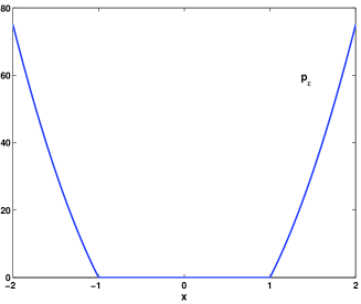
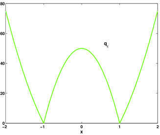
Figure 1: Profiles of potentials $p_{\epsilon}$ (left) and $q_{\epsilon}$ (right) versus $x$.

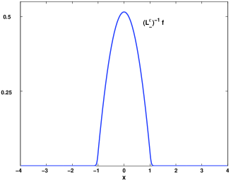
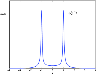
Figure 2: Schematic shapes of $(L_{-}^{\varepsilon})^{-1}f$ and $(L_{+}^{\varepsilon})^{-1}f$ for $f(x)=\exp(-x^{2}/4)\in L^{2}(\mathbb{R})$.

Lemma 2.5

Let $\alpha\in(0,+\infty]$ and $\delta>0$. Then for $0<\varepsilon\ll 1$,

$$\|\partial_{x}(L_{+}^{\varepsilon})^{-1}(L_{-}^{\varepsilon})^{-1}\|_{\mathcal{L}(L^{2}(\mathbb{R}))} \lesssim \varepsilon^{11/12},$$ (2.23)

$$\|(L_{+}^{\varepsilon})^{-1}(L_{-}^{\varepsilon})^{-1}\|_{\mathcal{L}(L^{2}(\mathbb{R}))} \lesssim \varepsilon^{26/15-\delta},$$ (2.24)

$$\|\mathbf{1}_{\{|x|>1\}}(L_{+}^{\varepsilon})^{-1}(L_{-}^{\varepsilon})^{-1}\|_{\mathcal{L}(L^{2}(\mathbb{R}))} \lesssim \varepsilon^{7/3-\delta},$$ (2.25)

$$\|\mathbf{1}_{\{|x|>1-\varepsilon^{\alpha}\}}\partial_{x}\left(L_{+}^{\varepsilon}\right)^{-1}\left(L_{-}^{\varepsilon}\right)^{-1}\|_{\mathcal{L}(L^{2}(\mathbb{R}),L^{\infty}(\mathbb{R}))} \lesssim \varepsilon^{\min\left(4/3,1/3+3\alpha/2\right)-\delta},$$ (2.26)

$$\|\mathbf{1}_{\{|x|>1-\varepsilon^{\alpha}\}}\left(L_{+}^{\varepsilon}\right)^{-1}\left(L_{-}^{\varepsilon}\right)^{-1}\|_{\mathcal{L}(L^{2}(\mathbb{R}),L^{\infty}(\mathbb{R}))} \lesssim \varepsilon^{\min\left(2,1+3\alpha/2\right)-\delta},$$ (2.27)

where if $\alpha=+\infty$, we use the convention $\varepsilon^{\alpha}=0$.

• Proof. Let $f\in B_{L^{2}}$, $S=(L_{-}^{\varepsilon})^{-1}f$ and $R=(L_{+}^{\varepsilon})^{-1}S$. We choose $\gamma\in(0,2/3)$ (in the sequel, we will make different explicit choices of such $\gamma$), and we split $R$ into three pieces: $R=R_{1}+R_{2}+R_{3}$, where

  $$R_{1} = (L_{+}^{\varepsilon})^{-1}\mathbf{1}_{\{|x|>1\}}(L_{-}^{\varepsilon})^{-1}f,$$

  $$R_{2} = (L_{+}^{\varepsilon})^{-1}\mathbf{1}_{\{1-\varepsilon^{\gamma}<|x|<1\}}(L_{-}^{\varepsilon})^{-1}f,$$

  $$R_{3} = (L_{+}^{\varepsilon})^{-1}\mathbf{1}_{(-1+\varepsilon^{\gamma},1-\varepsilon^{\gamma})}(L_{-}^{\varepsilon})^{-1}f.$$

  Notice that $R_{2}$ and $R_{3}$ depend on $\gamma$. According to Lemmas 2.2, 2.3 and 2.4,

  $$\|R_{1}^{\prime}\|_{L^{2}(\mathbb{R})}\lesssim\varepsilon^{5/3},\quad\|R_{1}\|_{L^{2}(\mathbb{R})}\lesssim\varepsilon^{7/3},\quad\|R_{1}^{\prime}\|_{L^{\infty}(\mathbb{R})}\lesssim\varepsilon^{4/3},\quad\|R_{1}\|_{L^{\infty}(\mathbb{R})}\lesssim\varepsilon^{2}.$$ (2.28)

  Thanks to Lemma 2.2, the Taylor formula provides

  $$\|S\|_{L^{2}(1-\varepsilon^{\gamma},1)}\lesssim\varepsilon^{\gamma/2}(|S(1)|+\varepsilon^{\gamma}\|S^{\prime}\|_{L^{\infty}(-1,1)})\lesssim\varepsilon^{\gamma/2}(\varepsilon^{2/3}+\varepsilon^{\gamma})\lesssim\varepsilon^{3\gamma/2},$$ (2.29)

  because $\gamma<2/3$. Thus, using Lemmas 2.3 and 2.4, we obtain

  $$\|R_{2}^{\prime}\|_{L^{2}(\mathbb{R})}\lesssim\varepsilon^{2/3+3\gamma/2},\|R_{2}\|_{L^{2}(\mathbb{R})}\lesssim\varepsilon^{4/3+3\gamma/2},\|R_{2}^{\prime}\|_{L^{\infty}(\mathbb{R})}\lesssim\varepsilon^{1/3+3\gamma/2},\|R_{2}\|_{L^{\infty}(\mathbb{R})}\lesssim\varepsilon^{1+3\gamma/2}.\ \$$ (2.30)

  The last component $R_{3}$ solves the differential equation

  $$L_{+}^{\varepsilon}R_{3}=\mathbf{1}_{(-1+\varepsilon^{\gamma},1-\varepsilon^{\gamma})}S,\qquad x\in\mathbb{R}.$$ (2.31)

  We multiply this equality by $R_{3}$, integrate over $\mathbb{R}$ and use the Cauchy-Schwarz inequality. Since $\|S\|_{L^{2}(\mathbb{R})}\lesssim 1$, we get

  $$\|R_{3}^{\prime}\|_{L^{2}(\mathbb{R})}^{2}+\int_{\mathbb{R}}q_{\varepsilon}|R_{3}|^{2}dx\lesssim\|R_{3}\|_{L^{2}(-1+\varepsilon^{\gamma},1-\varepsilon^{\gamma})}.$$ (2.32)

  Thus, since $\|R_{3}\|_{L^{2}(-1+\varepsilon^{\gamma},1-\varepsilon^{\gamma})}^{2}\lesssim\varepsilon^{2-\gamma}\int_{\mathbb{R}}q_{\varepsilon}|R_{3}|^{2}dx$,

  $$\|R_{3}^{\prime}\|_{L^{2}(\mathbb{R})}^{2}+\frac{1}{\varepsilon^{2-\gamma}}\left(\|R_{3}\|_{L^{2}(-1+\varepsilon^{\gamma},1-\varepsilon^{\gamma})}-C\varepsilon^{2-\gamma}\right)^{2}\lesssim\varepsilon^{2-\gamma}$$ (2.33)

  for some $C>0$. We deduce

  $$\|R_{3}^{\prime}\|_{L^{2}(\mathbb{R})}\lesssim\varepsilon^{1-\gamma/2},\qquad\|R_{3}\|_{L^{2}(-1+\varepsilon^{\gamma},1-\varepsilon^{\gamma})}\lesssim\varepsilon^{2-\gamma}.$$ (2.34)

  Next, we will establish an estimate on $\|R_{3}\|_{L^{2}(1-\varepsilon^{\gamma}<|x|<1)}$. We first estimate the $L^{\infty}(\mathbb{R})$ norm of $R_{3}$. Let $\chi$ be a $\mathcal{C}^{\infty}$ function on $\mathbb{R}$ with values in $[0,1]$ such that $\chi(x)\equiv 0$ for $x<-1/2$ and $\chi(x)\equiv 1$ for $x>0$. We denote $\widetilde{\chi R_{3}}$ the function defined by

  $$\widetilde{\chi R_{3}}(x):=\chi R_{3}\left(1-\varepsilon^{\gamma}+(x-1+\varepsilon^{\gamma})\varepsilon^{1-\gamma/2}\right).$$

  Then, using Sobolev’s embedding of $H^{1}(-\infty,1-\varepsilon^{\gamma})$ into $L^{\infty}(-\infty,1-\varepsilon^{\gamma})$ (notice that the norm of this embedding is the same that the norm of $H^{1}(\mathbb{R}_{+})\subset L^{\infty}(\mathbb{R}_{+})$, and therefore does not depend on $\varepsilon$), we obtain

  $$\|R_{3}\|_{L^{\infty}(0,1-\varepsilon^{\gamma})} \leqslant \|\chi R_{3}\|_{L^{\infty}(-\infty,1-\varepsilon^{\gamma})}\quad=\quad\|\widetilde{\chi R_{3}}\|_{L^{\infty}(-\infty,1-\varepsilon^{\gamma})}\quad\lesssim\quad\|\widetilde{\chi R_{3}}\|_{H^{1}(-\infty,1-\varepsilon^{\gamma})}$$ (2.35)

  $$\lesssim \varepsilon^{-1/2+\gamma/4}\|\chi R_{3}\|_{L^{2}(-\infty,1-\varepsilon^{\gamma})}+\varepsilon^{1/2-\gamma/4}\|(\chi R_{3})^{\prime}\|_{L^{2}(-\infty,1-\varepsilon^{\gamma})}$$

  $$\lesssim \varepsilon^{3/2-3\gamma/4}.$$

  Similarly, $\|R_{3}\|_{L^{\infty}(-1+\varepsilon^{\gamma},0)}\lesssim\varepsilon^{3/2-3\gamma/4}$. Since $R_{3}$ solves

  $$-\partial_{x}^{2}R_{3}+q_{\varepsilon}R_{3}=0,\quad|x|>1-\varepsilon^{\gamma},$$

  where $q_{\varepsilon}\geqslant 0$ and $R_{3}\in L^{2}(\mathbb{R})$, we infer from the maximum principle that

  $$\|R_{3}\|_{L^{\infty}(\mathbb{R})}\lesssim\varepsilon^{3/2-3\gamma/4}.$$ (2.36)

  On the interval $(1-\varepsilon^{\gamma},1)$, there exists constants $C_{A}^{\varepsilon}$ and $C_{B}^{\varepsilon}$ such that $R_{3}$ is given by the linear combination

  $$R_{3}=C_{A}^{\varepsilon}\psi_{A}^{\varepsilon}+C_{B}^{\varepsilon}\psi_{B}^{\varepsilon},$$

  where $\psi_{A}^{\varepsilon}$ and $\psi_{B}^{\varepsilon}$ are defined in Lemma 2.6 below.

  Lemma 2.6

  There exists a constant $C>0$ such that for $\varepsilon>0$ sufficiently small, the equation

  $$-\psi^{\prime\prime}(x)+\frac{2(1-x^{2})}{\varepsilon^{2}}\psi(x)=0,\quad-\frac{1}{2}<x<1$$ (2.37)

  has two linearly independent solutions $\psi_{A}^{\varepsilon}$ and $\psi_{B}^{\varepsilon}$ in the form

  $$\psi_{A}^{\varepsilon}(x)=a(1-x){\rm Ai}\left(\frac{\xi(1-x)}{\varepsilon^{2/3}}\right)\left(1+Q_{A}^{\varepsilon}(x)\right),$$

  $$\psi_{B}^{\varepsilon}(x)=a(1-x){\rm Bi}\left(\frac{\xi(1-x)}{\varepsilon^{2/3}}\right)\left(1+Q_{B}^{\varepsilon}(x)\right),$$

  where $\xi(x):=\left(\frac{3}{2}\int_{0}^{x}\sqrt{2t(2-t)}dt\right)^{2/3}$, $a(x):=\left(\xi^{\prime}(x)\right)^{-1/2}$, ${\rm Ai}$, ${\rm Bi}$ are the Airy functions, and $Q_{A}^{\varepsilon}$, $Q_{B}^{\varepsilon}$ satisfy the bound

  $$\|Q_{A}^{\varepsilon}\|_{L^{\infty}(-1/2,1)}+\|Q_{B}^{\varepsilon}\|_{L^{\infty}(-1/2,1)}\leqslant C\varepsilon^{2/3}.$$

• Proof. See Appendix A.3.  

According to 10.4.59 and 10.4.63 in [AS], the Airy functions satisfy the following asymptotic behaviour at infinity [AS, Section 10.4]:

$${\rm Ai}(z)\sim\frac{1}{2\pi^{1/2}z^{1/4}}e^{-\frac{2}{3}z^{3/2}}\quad\text{and}\quad{\rm Bi}(z)\sim\frac{1}{\pi^{1/2}z^{1/4}}e^{\frac{2}{3}z^{3/2}}\quad\text{as }z\to+\infty.$$ (2.38)

At the point $x=1$, we deduce from (2.36) that

$$\left|C_{A}^{\varepsilon}a(0){\rm Ai}(0)(1+Q_{A}^{\varepsilon}(1))+C_{B}^{\varepsilon}a(0){\rm Bi}(0)(1+Q_{B}^{\varepsilon}(1))\right|\lesssim\varepsilon^{3/2-3\gamma/4}.$$

Thus,

$$|C_{A}^{\varepsilon}|\lesssim\varepsilon^{3/2-3\gamma/4}+|C_{B}^{\varepsilon}|.$$ (2.39)

At the point $x=1-\varepsilon^{\gamma}$, provided that $\gamma<2/3$, we similarly have

$$\left|C_{A}^{\varepsilon}a(\varepsilon^{\gamma}){\rm Ai}\left(\frac{\xi(\varepsilon^{\gamma})}{\varepsilon^{2/3}}\right)(1+Q_{A}^{\varepsilon}(1-\varepsilon^{\gamma}))+C_{B}^{\varepsilon}a(\varepsilon^{\gamma}){\rm Bi}\left(\frac{\xi(\varepsilon^{\gamma})}{\varepsilon^{2/3}}\right)(1+Q_{B}^{\varepsilon}(1-\varepsilon^{\gamma}))\right|\lesssim\varepsilon^{3/2-3\gamma/4}.$$

Since

$$\xi(x)\sim 2^{2/3}x\quad\mbox{as}\quad x\to 0$$ (2.40)

and thanks to (2.38) and (2.39), we obtain

$$|C_{B}^{\varepsilon}|\lesssim\frac{\varepsilon^{3/2-3\gamma/4}}{{\rm Bi}\left(\frac{\xi(\varepsilon^{\gamma})}{\varepsilon^{2/3}}\right)}\quad\text{and}\quad|C_{A}^{\varepsilon}|\lesssim\varepsilon^{3/2-3\gamma/4},$$ (2.41)

where ${\rm Bi}\left(\frac{\xi(\varepsilon^{\gamma})}{\varepsilon^{2/3}}\right)\to\infty$ as $\varepsilon\to 0$. Since $\gamma<2/3$, one can choose $\beta\in(\gamma,1-\gamma/2)$. Using again the maximum principle, we get

$$|R_{3}(x)|\leqslant|R_{3}(1-\varepsilon^{\gamma}+\varepsilon^{\beta})|,\quad x>1-\varepsilon^{\gamma}+\varepsilon^{\beta}.$$

Moreover, thanks to (2.41), we have

$$|R_{3}(1-\varepsilon^{\gamma}+\varepsilon^{\beta})| \lesssim \varepsilon^{3/2-3\gamma/4}{\rm Ai}\left(\frac{\xi(\varepsilon^{\gamma}-\varepsilon^{\beta})}{\varepsilon^{2/3}}\right)+\varepsilon^{3/2-3\gamma/4}\frac{{\rm Bi}\left(\frac{\xi(\varepsilon^{\gamma}-\varepsilon^{\beta})}{\varepsilon^{2/3}}\right)}{{\rm Bi}\left(\frac{\xi(\varepsilon^{\gamma})}{\varepsilon^{2/3}}\right)}.$$

Using (2.40) again, we deduce from (2.38) that there exist a constant $c_{0}>0$ such that

$$\varepsilon^{3/2-3\gamma/4}{\rm Ai}\left(\frac{\xi(\varepsilon^{\gamma}-\varepsilon^{\beta})}{\varepsilon^{2/3}}\right)\lesssim\exp\left(-c_{0}\varepsilon^{3\gamma/2-1}\right),$$

$$\varepsilon^{3/2-3\gamma/4}\frac{{\rm Bi}\left(\frac{\xi(\varepsilon^{\gamma}-\varepsilon^{\beta})}{\varepsilon^{2/3}}\right)}{{\rm Bi}\left(\frac{\xi(\varepsilon^{\gamma})}{\varepsilon^{2/3}}\right)}\lesssim\exp\left(-c_{0}\varepsilon^{\beta+\gamma/2-1}\right),$$

where we have used

$$\frac{\xi(\varepsilon^{\gamma}-\varepsilon^{\beta})^{3/2}-\xi(\varepsilon^{\gamma})^{3/2}}{\varepsilon}\sim-3\varepsilon^{\beta+\gamma/2-1}\quad\text{as}\quad\varepsilon\to 0,$$

which holds because $\beta\in(\gamma,1-\gamma/2)$. Therefore, we find

$$\|R_{3}\|_{L^{\infty}(1-\varepsilon^{\gamma}+\varepsilon^{\beta},+\infty)}\lesssim|R_{3}(1-\varepsilon^{\gamma}+\varepsilon^{\beta})|\lesssim\exp\left(-c_{0}\varepsilon^{\beta+\gamma/2-1}\right),$$ (2.42)

which shows that $R_{3}(1)$ and $C_{A}^{\varepsilon}$ are actually exponentially decaying as $\varepsilon\to 0$. Then, we infer from (2.36) and (2.42)

$$\|R_{3}\|_{L^{2}(1-\varepsilon^{\gamma},1)} \lesssim \|R_{3}\|_{L^{2}(1-\varepsilon^{\gamma},1-\varepsilon^{\gamma}+\varepsilon^{\beta})}+\|R_{3}\|_{L^{2}(1-\varepsilon^{\gamma}+\varepsilon^{\beta},1)}$$ (2.43)

$$\lesssim \varepsilon^{\beta/2}\varepsilon^{3/2-3\gamma/4}+\varepsilon^{\gamma/2}\exp\left(-c_{0}\varepsilon^{\beta+\gamma/2-1}\right)\lesssim\varepsilon^{3/2+\beta/2-3\gamma/4}.$$

The $L^{2}$ norm of $R_{3}$ on the interval $(-1,-1+\varepsilon^{\gamma})$ is estimated in the same way. Next, we estimate the $L^{2}$ norm of $R_{3}$ on the interval $(1,\infty)$. We multiply (2.31) by $R_{3}$ and integrate over $(1,+\infty)$. Since $p_{\varepsilon}\geqslant 1$ for $x\geqslant 2$ and $\varepsilon\leqslant 1$, we obtain

$$\|R_{3}\|_{L^{2}(2,+\infty)}^{2}\leqslant\int_{1}^{+\infty}(R_{3}^{\prime})^{2}dx+\int_{1}^{+\infty}p_{\varepsilon}R_{3}^{2}dx = -R_{3}(1)R_{3}^{\prime}(1)$$ (2.44)

$$\lesssim \exp\left(-c_{0}\varepsilon^{\beta+\gamma/2-1}\right)\varepsilon^{1/3},$$

where $R_{3}(1)$ has been estimated with (2.42) and the bound for $R_{3}^{\prime}(1)$ comes from Lemmas 2.4 and 2.1. The $L^{2}$ norm of $R_{3}$ on $(1,2)$ is estimated thanks to (2.42). Together with (2.44), we deduce that

$$\|R_{3}\|_{L^{2}(1,+\infty)}\lesssim\exp\left(-c\varepsilon^{\beta+\gamma/2-1}\right),$$

where $c=c_{0}/2$. The $L^{2}$ norm of $R_{3}$ on $(-\infty,-1)$ is estimated similarly, thus

$$\|R_{3}\|_{L^{2}(|x|>1)}\lesssim\exp\left(-c\varepsilon^{\beta+\gamma/2-1}\right).$$ (2.45)

Since $R_{3}$ solves

$$-R_{3}^{\prime\prime}+q_{\varepsilon}R_{3}=0$$

on $(1-\varepsilon^{\gamma},+\infty)$ and $R_{3}\in L^{2}(\mathbb{R})$, we deduce from the maximum principle that if $R_{3}$ does not identically vanish on $(1-\varepsilon^{\gamma},+\infty)$, then $R_{3}$ has a constant sign on that interval. For instance, $R_{3}>0$ (the argument is similar in the other case). Then, $R_{3}^{\prime\prime}(x)\geqslant 0$ for every $x\geqslant 1-\varepsilon^{\gamma}$. Therefore $R_{3}^{\prime}$ is a negative increasing function on $(1-\varepsilon^{\gamma},+\infty)$. Let us assume by contradiction that $\left|R_{3}^{\prime}(1-\varepsilon^{\gamma}+\varepsilon^{\beta})\right|>\exp(-c_{0}\varepsilon^{\beta+\gamma/2-1})/\varepsilon^{2}$. Then, for $x\geqslant 0$, it follows from the Taylor formula and (2.42) that for $\varepsilon$ sufficiently small,

$$R_{3}(1-\varepsilon^{\gamma}+\varepsilon^{\beta}+\varepsilon) = R_{3}(1-\varepsilon^{\gamma}+\varepsilon^{\beta})+\varepsilon R_{3}^{\prime}(1-\varepsilon^{\gamma}+\varepsilon^{\beta})+\int_{0}^{\varepsilon}\int_{0}^{s}R_{3}^{\prime\prime}(1-\varepsilon^{\gamma}+\varepsilon^{\beta}+t)dtds$$

$$\leqslant \exp(-c_{0}\varepsilon^{\beta+\gamma/2-1})\left(C-\frac{\varepsilon}{\varepsilon^{2}}+C\frac{\varepsilon^{2}}{2}\frac{1}{\varepsilon^{2-\gamma}}\right)<0,$$

for some $C>0$, which is a contradiction with the positiveness of $R_{3}$. As a result,

$$\|R_{3}^{\prime}\|_{L^{\infty}(1-\varepsilon^{\gamma}+\varepsilon^{\beta},+\infty)}=\left|R_{3}^{\prime}(1-\varepsilon^{\gamma}+\varepsilon^{\beta})\right|\lesssim\exp(-c\varepsilon^{\beta+\gamma/2-1}).$$ (2.46)

At this stage, we have established all the estimates required to prove the lemma. First, (2.28), (2.30) and (2.34) yield

$$\|R^{\prime}\|_{L^{2}(\mathbb{R})} \leqslant \|R^{\prime}_{1}\|_{L^{2}(\mathbb{R})}+\|R^{\prime}_{2}\|_{L^{2}(\mathbb{R})}+\|R^{\prime}_{3}\|_{L^{2}(\mathbb{R})}$$ (2.47)

$$\lesssim \varepsilon^{5/3}+\varepsilon^{2/3+3\gamma/2}+\varepsilon^{1-\gamma/2}.$$

The choice $\gamma=1/6$ provides (2.23). From (2.28), (2.30), (2.34), (2.43) and (2.45), we obtain

$$\|R\|_{L^{2}(\mathbb{R})} \leqslant \|R_{1}\|_{L^{2}(\mathbb{R})}+\|R_{2}\|_{L^{2}(\mathbb{R})}+\|R_{3}\|_{L^{2}(-1+\varepsilon^{\gamma},1-\varepsilon^{\gamma})}+\|R_{3}\|_{L^{2}(1-\varepsilon^{\gamma}<|x|<1)}+\|R_{3}\|_{L^{2}(|x|>1)}$$ (2.48)

$$\lesssim \varepsilon^{7/3}+\varepsilon^{4/3+3\gamma/2}+\varepsilon^{2-\gamma}+\varepsilon^{3/2-3\gamma/4+\beta/2}+\exp\left(-c\varepsilon^{\beta+\gamma/2-1}\right).$$

The choice $\gamma=4/15$, $\beta=13/15-2\delta$, for sufficiently small positive number $\delta$, provides the bound (2.24). Similarly, we have

$$\|R\|_{L^{2}(|x|>1)} \leqslant \|R_{1}\|_{L^{2}(|x|>1)}+\|R_{2}\|_{L^{2}(|x|>1)}+\|R_{3}\|_{L^{2}(|x|>1)}$$ (2.49)

$$\lesssim \varepsilon^{7/3}+\varepsilon^{4/3+3\gamma/2}+\exp\left(-c\varepsilon^{\beta+\gamma/2-1}\right).$$

The choice $\gamma=2(1-\delta)/3$, $\beta=2/3$, for any small positive number $\delta$, provides the bound (2.25). If $\alpha>0$, $\gamma<\min(\alpha,2/3)$ and if $\varepsilon$ is sufficiently small, we also obtain from (2.28), (2.30) and (2.46),

$$\|R^{\prime}\|_{L^{\infty}(1-\varepsilon^{\alpha},+\infty)}\leqslant\|R^{\prime}\|_{L^{\infty}(1-\varepsilon^{\gamma}+\varepsilon^{\beta},+\infty)} \leqslant \|R^{\prime}_{1}\|_{L^{\infty}(\mathbb{R})}+\|R^{\prime}_{2}\|_{L^{\infty}(\mathbb{R})}+\|R^{\prime}_{3}\|_{L^{\infty}(1-\varepsilon^{\gamma}+\varepsilon^{\beta},+\infty)}$$ (2.50)

$$\lesssim \varepsilon^{4/3}+\varepsilon^{1/3+3\gamma/2}+\exp\left(-c\varepsilon^{\beta+\gamma/2-1}\right).$$

A similar argument on $(-\infty,-1+\varepsilon^{\alpha})$ gives (2.26), for the choice $\gamma=\min(\alpha,2/3)-2\delta/3$, $\beta=(1+\gamma)/4$. If $\gamma<\min(\alpha,2/3)$, thanks to (2.28), (2.30), (2.42) and its twin estimate on $(-\infty,-1+\varepsilon^{\alpha})$, we get similarly, for $\varepsilon$ sufficiently small,

$$\|R\|_{L^{\infty}(|x|>1-\varepsilon^{\alpha})}\leqslant\|R\|_{L^{\infty}(|x|>1-\varepsilon^{\gamma}+\varepsilon^{\beta})} \lesssim \|R_{1}\|_{L^{\infty}(\mathbb{R})}+\|R_{2}\|_{L^{\infty}(\mathbb{R})}+\|R_{3}\|_{L^{\infty}(|x|>1-\varepsilon^{\gamma}+\varepsilon^{\beta})}$$ (2.51)

$$\lesssim \varepsilon^{2}+\varepsilon^{1+3\gamma/2}+\exp\left(-c_{0}\varepsilon^{\beta+\gamma/2-1}\right).$$

The bound (2.27) follows from (2.51), again with the choice $\gamma=\min(\alpha,2/3)-2\delta/3$, $\beta=(1+\gamma)/4$.  

3 Proof of the Main Theorem

3.1 The operator $A_{\varepsilon}$ for $\varepsilon>0$

We consider here the operator

$$A_{\varepsilon}:=\varepsilon^{-2}(-\partial_{x}^{2}+p_{\varepsilon}(x))^{-1}(-\partial_{x}^{2}+q_{\varepsilon}(x))^{-1}=\varepsilon^{-2}(L_{-}^{\varepsilon})^{-1}(L_{+}^{\varepsilon})^{-1}.$$ (3.1)

As we have seen before, if $\varepsilon>0$, both operators $L_{-}^{\varepsilon}$ and $L_{+}^{\varepsilon}$ on $L^{2}(\mathbb{R})$ are invertible with compact resolvent. As a result, $A_{\varepsilon}$ is a compact operator on $L^{2}(\mathbb{R})$ for any fixed $\varepsilon>0$. Thus, its spectrum consists of a sequence of eigenvalues which converges to zero. Moreover, these eigenvalues are all strictly positive. Indeed, if $\mu$ is an eigenvalue of $A_{\varepsilon}$ and $\varphi$ is an associated eigenvector, $\zeta:=(L_{+}^{\varepsilon})^{-1/2}\varphi$ satisfies

$$(L_{+}^{\varepsilon})^{-1/2}(L_{-}^{\varepsilon})^{-1}(L_{+}^{\varepsilon})^{-1/2}\zeta=\mu\zeta.$$

Therefore, $\mu$ is an eigenvalue of the self adjoint positive operator $(L_{+}^{\varepsilon})^{-1/2}(L_{-}^{\varepsilon})^{-1}(L_{+}^{\varepsilon})^{-1/2}$, which implies $\mu>0$. We order eigenvalues of $A_{\varepsilon}$ as

$$0<\cdots\leqslant\mu_{n,\varepsilon}\leqslant\cdots\leqslant\mu_{2,\varepsilon}\leqslant\mu_{1,eps}<\infty.$$

3.2 The operator $A_{0}$

As $\varepsilon\to 0$, we can formally expect that $A_{\varepsilon}$ converges in some sense to the operator

$$A_{0}=(-\partial_{x}^{2}+p_{0})^{-1}\frac{1}{2(1-x^{2})},$$

where

$$p_{0}(x)=\left\{\begin{array}[]{ll}0&\text{if }|x|<1,\\ +\infty&\text{if }|x|>1.\end{array}\right.$$

Let us describe more precisely the action of the operator $A_{0}$ on $L^{2}(\mathbb{R})$. The following lemma is helpful for that purpose.

Lemma 3.1

If $u\in L^{2}(\mathbb{R})$, then $\left(\frac{u}{1-x^{2}}\right)_{|(-1,1)}\in\left(H^{2}\cap H_{0}^{1}\right)^{\prime}(-1,1)$, where $\left(H^{2}\cap H_{0}^{1}\right)(-1,1)$ is endowed with the $H^{2}$ norm. Moreover, the map $u\mapsto\left(\frac{u}{1-x^{2}}\right)_{|(-1,1)}$ is continuous from $L^{2}(\mathbb{R})$ into $\left(H^{2}\cap H_{0}^{1}\right)^{\prime}(-1,1)$.

• Proof. By Sobolev’s embedding theorem, $H^{2}(-1,1)$ is continuously embedded into $\mathcal{C}^{1}([-1,1])$. Therefore, if $g\in(H^{2}\cap H_{0}^{1})(-1,1)$, then

  $$|g(x)|=|g(x)-g(\pm 1)|\leqslant\|g^{\prime}\|_{L^{\infty}}(1-|x|),$$

  with $+1$ for $x>0$ and $-1$ for $x<0$. It follows that for every $x\in(-1,1)$,

  $$\left|\frac{g(x)}{1-x^{2}}\right|\leqslant\frac{\|g^{\prime}\|_{L^{\infty}}}{1+|x|}\lesssim\|g\|_{H^{2}}.$$

  As a result, using the Cauchy-Schwarz inequality, we obtain

  $$\left|\int_{-1}^{1}\frac{u(x)}{1-x^{2}}g(x)dx\right|\lesssim\|u\|_{L^{2}(\mathbb{R})}\|g\|_{H^{2}(-1,1)},$$

  which completes the proof.  

Let us denote the Dirichlet realization of the Laplacian $\Delta=\partial_{x}^{2}$ on the interval $(-1,1)$ by $\Delta_{D}$. It is well known that $(-\Delta_{D})^{-1}$ maps continuously $L^{2}(-1,1)$ into $\left(H^{2}\cap H_{0}^{1}\right)(-1,1)$. By duality, it also continuously maps $\left(H^{2}\cap H_{0}^{1}\right)^{\prime}(-1,1)$ into $L^{2}(-1,1)$. For $u\in L^{2}(\mathbb{R})$, $A_{0}u\in L^{2}(\mathbb{R})$ is defined by

$$\left\{\begin{array}[]{l}(A_{0}u)_{|\{|x|>1\}}\equiv 0,\\ (A_{0}u)_{|(-1,1)}=(-\Delta_{D})^{-1}\left(\left(\frac{u}{2(1-x^{2})}\right)_{|(-1,1)}\right).\end{array}\right.$$ (3.4)

Thanks to Lemma 3.1 and the continuity of $(-\Delta_{D})^{-1}:\left(H^{2}\cap H_{0}^{1}\right)^{\prime}(-1,1)\mapsto L^{2}(-1,1)$, $A_{0}$ is a bounded operator on $L^{2}(\mathbb{R})$. Moreover, we have the following lemma.

Lemma 3.2

For any $u\in L^{2}(\mathbb{R})$ and any $s\in[-1,1]$,

$$A_{0}u(s) = \int_{s}^{1}\left(\int_{-1}^{y}\frac{u(x)}{4(1-x)}dx-\int_{y}^{1}\frac{u(x)}{4(1+x)}dx\right)dy+\frac{s-1}{2}I(u),$$ (3.5)

where

$$I(u) := \int_{-1}^{1}\left(\int_{-1}^{y}\frac{u(x)}{4(1-x)}dx-\int_{y}^{1}\frac{u(x)}{4(1+x)}dx\right)dy.$$ (3.6)

In particular, $A_{0}u$ is continuous on $\mathbb{R}$.

• Proof. For any $u\in L^{2}(\mathbb{R})$ and any $y\in(-1,1]$, we have

  $$\left|\int_{y}^{1}\frac{u(x)}{(1+x)}dx\right|\leqslant\left(\int_{y}^{1}|u(x)|^{2}dx\right)^{1/2}\left(\int_{y}^{1}\frac{1}{(1+x)^{2}}dx\right)^{1/2}\leqslant\frac{\|u\|_{L^{2}(\mathbb{R})}}{\sqrt{1+y}},$$ (3.7)

  which implies that the map $u\mapsto\int_{y}^{1}\frac{u(x)}{1+x}dx$ is continuous from $L^{2}(\mathbb{R})$ into $L^{1}(-1,1)$. Similarly, one can see that the map $u\mapsto\int_{-1}^{y}\frac{u(x)}{1-x}dx$ has the same property. As a result, $u\mapsto I(u)$ is a continuous linear form on $L^{2}(\mathbb{R})$, and the map which assigns to $u$ the right hand side in (3.5) is continuous from $L^{2}(\mathbb{R})$ into $L^{\infty}(-1,1)\subset L^{2}(-1,1)$. As we have seen before, so is $u\mapsto(A_{0}u)_{|(-1,1)}$. Actually, both sides in (3.5) only depend on the restriction of $u$ to $(-1,1)$, so that they can be considered as continuous from $L^{2}(-1,1)$ into itself. Therefore, using the principle of extension for uniformly continuous functions, it suffices to check (3.5) for $u$ in a dense subset of $L^{2}(-1,1)$. This can be done for $u\in\mathcal{C}_{c}^{\infty}(-1,1)$. Indeed, in this case $\left(\frac{u}{1-x^{2}}\right)_{|(-1,1)}\in L^{2}(-1,1)$, therefore $(A_{0}u)_{|(-1,1)}\in\left(H^{2}\cap H_{0}^{1}\right)(-1,1)$. In particular, $\underset{s\to\pm 1\mp 0}{\lim}(A_{0}u)(s)=0$. On the other side, we can easily check that the right hand side in (3.5) also vanishes at $s=\pm 1$ and its second derivative is $-\frac{u(x)}{2(1-x^{2})}$, which completes the proof of (3.5). It remains to prove that $\underset{s\to\pm 1\mp 0}{\lim}(A_{0}u)(s)=0$ is true for any $u\in L^{2}(\mathbb{R})$. This follows from the fact that the maps $y\mapsto\int_{y}^{1}\frac{u(x)}{1+x}dx$ and $y\mapsto\int_{-1}^{y}\frac{u(x)}{1-x}dx$ are in $L^{1}(-1,1)$.  

Lemma 3.3

$A_{0}$ is a compact operator on $L^{2}(\mathbb{R})$.

• Proof. By Lemma 3.2, $A_{0}$ is continuous. Thus, according to a standard criterion of relative compactness for a subset of $L^{2}(\mathbb{R})$ (see, for instance, Corollary IV.26 in [B]), it is sufficient to check the following two conditions

  1. for every $\eta>0$, there exists a compact subset $\omega\subset\mathbb{R}$ such that for every $u\in B_{L^{2}}$,

     $$\|A_{0}u\|_{L^{2}(\mathbb{R}\\omega)}<\eta$$

  2. for every $\eta>0$ and for every compact subset $\omega\subset\mathbb{R}$, there exists $\delta>0$ such that for every $u\in B_{L^{2}}$ and for every $h$ with $|h|<\delta$,

     $$\|A_{0}u(\cdot+h)-A_{0}u\|_{L^{2}(\omega)}<\eta.$$

  In our case, condition (i) is trivially satisfied: we choose $\omega=[-1,1]$ and then $\|A_{0}u\|_{L^{2}(\mathbb{R}\\omega)}=0$ for every $u\in B_{L^{2}}$. To check condition (ii), we note that if $-1\leqslant s,s+h\leqslant 1$, then

  $$\left|A_{0}u(s+h)-A_{0}u(s)\right| = \left|-\int_{s}^{s+h}\left(\int_{-1}^{y}\frac{u(x)}{4(1-x)}dx-\int_{y}^{1}\frac{u(x)}{4(1+x)}dx\right)dy+\frac{h}{2}I(u)\right|$$

  $$\leqslant \left|\int_{s}^{s+h}\frac{\|u\|_{L^{2}(\mathbb{R})}}{4}\left(\frac{1}{\sqrt{1+y}}+\frac{1}{\sqrt{1-y}}\right)dy\right|+\frac{|h|}{2}C\|u\|_{L^{2}(\mathbb{R})}$$

  $$\leqslant \frac{\sqrt{|h|}}{4}+\frac{C|h|}{2},$$

  for some constant $C>0$. A similar estimate holds if either $+1$ or $-1$ lies between $s$ and $s+h$ (which can only happen if $|s|<1+|h|$), whereas if both $s$ and $s+h$ are outside of $(-1,1)$, then $A_{0}u(s+h)-A_{0}u(s)=0$. Therefore,

  $$\|A_{0}u(\cdot+h)-A_{0}u\|_{L^{2}(\mathbb{R})}\leqslant\left(2(1+|h|)\right)^{1/2}\left(\frac{\sqrt{|h|}}{4}+\frac{C|h|}{2}\right),$$

  and condition (ii) follows.  

Since $A_{0}$ is compact, its spectrum is purely discrete. Clearly, $0$ is an eigenvalue of $A_{0}$ and the associated infinite-dimensional eigenspace is made of the set of functions in $L^{2}(\mathbb{R})$ supported in the exterior domain $\{x\in\mathbb{R}:\;|x|\geqslant 1\}$. If $\mu\neq 0$ is an eigenvalue of $A_{0}$ and $w$ an associated eigenvector, it follows from the definition of $A_{0}$ that $w\equiv 0$ on $\{x\in\mathbb{R}:\;|x|\geqslant 1\}$, whereas on $\{x\in\mathbb{R}:\;|x|<1\}$, $w$ solves

$$-2(1-x^{2})w^{\prime\prime}(x)=\gamma w(x),\quad-1<x<1,$$ (3.8)

where $\gamma=1/\mu$. Moreover, thanks to Lemma 3.2, $w=\gamma A_{0}w$ is continuous so that $w(-1)=w(1)=0$. We shall now prove that the only solutions of (3.8) vanishing at the endpoints $\pm 1$ are the Gegenbauer polynomials $C_{n+1}^{-1/2}(x)$ for $\gamma_{n}=2n(n+1)$, where $n\geqslant 1$ is integer. Thus, the spectrum of operator $A_{0}$ is given by

$$\sigma(A_{0})=\left\{\mu_{n}:=\frac{1}{2n(n+1)},\;\;n\geqslant 1\right\}\cup\{0\}.$$

Lemma 3.4

Equation (3.8) admits a family of solutions $(\gamma,w)=(\gamma_{n},C_{n+1}^{-1/2})$, for $n\geqslant-1$, where $\gamma_{n}=2n(n+1)$ and $C_{m}^{\lambda}$ is a Gegenbauer polynomial with degree $m$. If $(\gamma,w)\not\in\{(\gamma_{n},\alpha C_{n+1}^{-1/2})\ |\ n\geqslant-1,\alpha\in\mathbb{R}\}$ is a solution of (3.8), then it satisfies

$$\lim_{x\to 1-0}\left(|w(x)|+|w(-x)|\right)\neq 0,\quad\lim_{x\to 1-0}\left(|w^{\prime}(x)|+|w^{\prime}(-x)|\right)=\infty.$$ (3.9)

The only solutions $(\gamma,w)$ of (3.8) such that $w(1)=w(-1)=0$ are $(\gamma_{n},\alpha C_{n+1}^{-1/2})$, for $n\geqslant 1$ and $\alpha\in\mathbb{R}$.

• Proof. Explicit computations show that Gegenbauer polynomials $C_{n+1}^{-1/2}(x)$ from Section 8.93 in [GR] are solutions of (3.8) for $\gamma_{n}$, for any $n\geqslant-1$. In particular, for $n\geqslant 1$, by equation 8.935 in [GR], we have

  $$C_{n+1}^{-1/2}(x)=-\frac{(1-x^{2})}{n(n+1)}\frac{d^{2}}{dx^{2}}C_{n+1}^{-1/2}(x)=\frac{(1-x^{2})}{n(n+1)}C_{n-1}^{3/2}(x),$$

  which proves that $C_{n+1}^{-1/2}(1)=C_{n+1}^{-1/2}(-1)=0$ for $n\geqslant 1$, whereas $C_{0}^{-1/2}(x)=1$ and $C_{1}^{-1/2}(x)=-x$. We next prove that if $(\gamma,w)$ solves (3.8) and $w$ is not proportional to $C_{n+1}^{-1/2}$ with $n\geqslant-1$, then $w$ satisfies (3.9). We introduce the new variable $z=x^{2}$ for $0<x<1$, and the function $u(z):=w(x)$. It is equivalent for $w(x)$ to solve (3.8) on $(0,1)$ or for $u(z)$ to solve the hypergeometric equation:

  $$z(1-z)u^{\prime\prime}(z)+\frac{1}{2}(1-z)u^{\prime}(z)+\frac{\gamma}{8}u(z)=0,\quad 0<z<1.$$ (3.10)

  This equation admits a general solution given by 9.152 in [GR]

  $$u(z)=c_{1}F(a,b,c;z)+c_{2}z^{1/2}F\left(a+\frac{1}{2},b+\frac{1}{2},\frac{3}{2};z\right),$$ (3.11)

  where

  $$a+b=-\frac{1}{2},\;\;ab=-\frac{\gamma}{8},\;\;c=\frac{1}{2}$$

  and $F(a,b,c;z)$ is a hypergeometric function. Clearly, the function $x\mapsto u(x^{2})=w(x)$ defined by (3.11) is analytic for $0<x<1$ and can be extended into an function $\tilde{w}$ which is analytic for $-1<x<1$, given by

  $$\tilde{w}(x) := c_{1}F(a,b,c;x^{2})+c_{2}xF\left(a+\frac{1}{2},b+\frac{1}{2},\frac{3}{2};x^{2}\right),$$

  where the first term is even in $x$ and the second term is odd in $x$. Since $\tilde{w}$ solves (3.10), the uniqueness in the Cauchy-Lipshitz Theorem ensures that $w=\tilde{w}$. In order to prove the Lemma, it is sufficient to consider one component of the solution at one boundary point, e.g. $F(a,b,c;x^{2})$ at $x=1$ ($z=1$). Since ${\rm Re}(c-a-b)=1>0$, the function $F(a,b,c;z)$, which is analytic on $\{z:|z|<1\}$, is also bounded as $z\to 1$ (see 15.1.1 in [AS]). Using 15.1.20 in [AS], that is

  $$F(a,b,c;1)=\frac{\Gamma(c)\Gamma(c-a-b)}{\Gamma(c-a)\Gamma(c-b)},$$

  we find that

  $$F(a,b,c;1)=\frac{\pi^{1/2}}{\Gamma(1+a)\Gamma(1/2-a)}=-\frac{\sin(\pi a)\Gamma(-a)}{\pi^{1/2}\Gamma(1/2-a)}=\frac{\cos(\pi a)\Gamma(1/2+a)}{\pi^{1/2}\Gamma(1+a)}.$$

  Parameters $a$ and $\gamma$ are related by $\gamma=4a(1+2a)$. If $\gamma=\gamma_{2m-1}=4m(2m-1)$ for $m\geqslant 1$, then either $a=-m$ or $a=-1/2+m$, both give $F(a,b,c;1)=0$, corresponding to even polynomial solutions $C_{2m}^{-1/2}$. For all other values of $\gamma$ and $a$, $F(a,b,c;1)$ is bounded but non-zero. On the other hand, using 15.2.1 in [AS], that is

  $$\frac{d}{dz}F(a,b,c;z)=\frac{ab}{c}F(a+1,b+1,c+1;z),$$

  since ${\rm Re}(c+1-a-1-b-1)=0$, we obtain that $\frac{d}{dx}F(a,b,c;z)=2x\frac{d}{dz}F(a,b,c;z)$ diverges as $z\to 1$ (see 15.1.1 in [AS]), unless the series for $F(a,b,c,z)$ is truncated into a polynomial function, which happens precisely when $a$ or $b$ is a negative integer, which implies that $\gamma$ equals one of the $\gamma_{2m-1}$’s for some $m\geqslant 0$. Therefore, $\lim_{x\to 1}|w^{\prime}(x)|=\infty$ if $w(x)$ is an even solution of (3.8) and $\gamma\neq\gamma_{2m-1}$ for $m\geqslant 0$. Similarly, the statement is proved for an odd solution of (3.8), given by $xF\left(a+1/2,b+1/2,3/2;x^{2}\right)$ for $\gamma\neq\gamma_{2m}$ with $m\geqslant 0$, where $\gamma=\gamma_{2m}=4m(2m+1)$ correspond to odd polynomial solutions $C_{2m-1}^{-1/2}$.  

3.3 Convergence in norm of $A_{\varepsilon}$ to $A_{0}$ as $\varepsilon\to 0$

Our goal in this section is to prove the following result.

Theorem 3.5

It is true that

$$A_{\varepsilon}\longrightarrow A_{0}\quad\text{in $\mathcal{L}(L^{2}(\mathbb{R}))$ as }\varepsilon\to 0.$$

Once this result has been proved, we immediately have the corollary.

Corollary 3.6

For every integer $n\geqslant 1$,

$$\mu_{n,\varepsilon}\longrightarrow\mu_{n}\quad\text{as }\varepsilon\to 0.$$

Moreover, if $w_{n}$ is an eigenvector of $A_{0}$ associated to the eigenvalue $\mu_{n}$, there exists a set $(w_{n,\varepsilon})_{\varepsilon>0}\subset L^{2}(\mathbb{R})$ of eigenvectors of $A_{\varepsilon}$ associated to the eigenvalues $\mu_{n,\varepsilon}$ for $\varepsilon>0$, such that

$$w_{n,\varepsilon}\longrightarrow w_{n}\quad\text{in }L^{2}(\mathbb{R})\text{ as }\varepsilon\to 0.$$

• Proof. Since convergence in norm in $\mathcal{L}(L^{2})$ implies generalized convergence, it follows from Theorem 3.16 on p.212 in [K] that for every integer $N\geqslant 1$ and for $0<\varepsilon\ll 1$,

  $$\left|\left(\frac{\mu_{N}+\mu_{N+1}}{2},+\infty\right)\cap\sigma(A_{\varepsilon})\right|=N.$$

  Moreover, $\mu_{n,\varepsilon}\to\mu_{n}$ as $\varepsilon\to 0$, for any $1\leqslant n\leqslant N$, which proves the convergence of the eigenvalues. For the eigenvectors, let us fix $n\geqslant 1$, and let $\Omega_{n}\subset\mathbb{C}$ be a neighborhood of $\mu_{n}$ such that $\overline{\Omega_{n}}$ does not contain 0 nor any other eigenvalue of $A_{0}$. From the convergence of the eigenvalues, it follows that for $\varepsilon$ sufficiently small, $A_{\varepsilon}$ has a unique eigenvalue in $\Omega_{n}$, which is $\mu_{n,\varepsilon}$. For any integer $m\geqslant 1$, we denote by $E_{m}$ (resp. $E_{m}^{\varepsilon}$) the eigenspace of $A_{0}$ (resp $A_{\varepsilon}$) associated to the eigenvalue $\mu_{m}$ (resp $\mu_{m,\varepsilon}$). We also define

  $$F_{n}:=\left(\underset{m\neq n}{\oplus}E_{m}\right){\oplus}{\rm Ker}A_{0}\quad\text{ and }\quad F_{n,\varepsilon}:=\underset{m\neq n}{\oplus}E_{m}^{\varepsilon},$$

  as well as $P_{n}\in\mathcal{L}(L^{2}(\mathbb{R}))$ (resp. $P_{n,\varepsilon}$) the projector on $E_{n}$ (resp $E_{n,\varepsilon}$) along $F_{n}$ (resp. $F_{n,\varepsilon}$). Then, Theorem 3.16 in [K] also ensures that $P_{n,\varepsilon}\longrightarrow P_{n}$ in $\mathcal{L}(L^{2})$ as $\varepsilon\to 0$. Thus, $w_{n,\varepsilon}:=P_{n,\varepsilon}w_{n}$ is an eigenvector of $A_{\varepsilon}$ for the eigenvalue $\mu_{n,\varepsilon}$, and we have

  $$\|w_{n,\varepsilon}-w_{n}\|_{L^{2}(\mathbb{R})}=\|(P_{n,\varepsilon}-P_{n})w_{n}\|_{L^{2}(\mathbb{R})}\leqslant\|P_{n,\varepsilon}-P_{n}\|_{\mathcal{L}(L^{2}(\mathbb{R}))}\|w_{n}\|_{L^{2}(\mathbb{R})}\underset{\varepsilon\to 0}{\longrightarrow}0,$$

  which completes the proof.  

Remark 3.7

A straightforward consequence of Theorem 3.5 is that $A_{\varepsilon}^{*}\to A_{0}^{*}$ in $\mathcal{L}(L^{2}(\mathbb{R}))$ as $\varepsilon\to 0$. Thus, an analogous result to Corollary 3.6 holds for the eigenvalues and eigenvectors of $A_{\varepsilon}^{*}$ and $A_{0}^{*}$.

The convergence statement of the Main Theorem directly follows from Corollary 3.6, since the spectrum of system (1.7) is made is made of the eigenvalues $\lambda=\pm i\varepsilon/\sqrt{\mu}$, where $\mu$ describes the spectrum $\sigma(A_{\varepsilon})$ of $A_{\varepsilon}$. Indeed, if $(\lambda,u,w)\in\mathbb{C}\times L^{2}(\mathbb{R})\times L^{2}(\mathbb{R})$ solves (1.7), a straightforward computation shows that

$$A_{\varepsilon}w=-\frac{\varepsilon^{2}}{\lambda^{2}}w,$$

thus $\lambda=\pm\frac{i\varepsilon}{\sqrt{\mu}}$ for some $\mu\in\sigma(A_{\varepsilon})$. Conversely, if $A_{\varepsilon}w=\mu w,$ with $w\in L^{2}(\mathbb{R})$, then $(i\varepsilon/\sqrt{\mu},u,w)\in\mathbb{C}\times L^{2}(\mathbb{R})\times L^{2}(\mathbb{R})$ solves system (1.7) with

$$u:=-\frac{i}{\varepsilon\sqrt{\mu}}(L_{+}^{\varepsilon})^{-1}w.$$

Let us now turn to the proof of Theorem 3.5. In order to compare $A_{0}u$ and $A_{\varepsilon}u$ for $\varepsilon>0$ and $u\in L^{2}(\mathbb{R})$, we would like first to express $A_{0}u$ as $A_{0}u=A_{\varepsilon}(A_{\varepsilon})^{-1}A_{0}u$. This can be done with the help of the following lemma.

Lemma 3.8

Let $H$ be a Hilbert space and $L$ be a self-adjoint operator on $H$ with domain $D(L)$ endowed with the graph-norm $\|\cdot\|_{D(L)}=\left(\|\cdot\|_{H}^{2}+\|L\cdot\|_{H}^{2}\right)^{1/2}$. Assume that $L$ is continuously invertible and $X$ is a Banach space continuously embedded in $H$. $L$ induces an operator $L_{X}$ on $X$, defined by

$$D(L_{X})=\{x\in X,\ \ L_{X}x\in X\},\quad L_{X}x=Lx\quad\text{for any }x\in D(L_{X}).$$

$D(L_{X})$ is endowed with the graph-norm $\|\cdot\|_{D(L_{X})}=\left(\|\cdot\|_{X}^{2}+\|L_{X}\cdot\|_{X}^{2}\right)^{1/2}$. Assume further that $D(L_{X})$ is dense in $H$ and that $D(L)$ is continuously embedded in $X$. Then $L$ is extended to $X^{\prime}$ as a bicontinuous map $L_{X^{\prime}}:X^{\prime}\mapsto D(L_{X})^{\prime}$ defined by

$$\left<L_{X^{\prime}}f,\varphi\right>_{D(L_{X})^{\prime},D(L_{X})}:=\left<f,L_{X}\varphi\right>_{X^{\prime},X}\quad\text{for any }f\in X^{\prime}\text{ and }\varphi\in D(L_{X}).$$

• Proof. See Appendix A.4.  

To prove that $A_{0}u=A_{\varepsilon}(A_{\varepsilon})^{-1}A_{0}u$ for any $\varepsilon>0$ and $u\in L^{2}(\mathbb{R})$, we apply Lemma 3.8 twice. For the first application, $H=X=L^{2}(\mathbb{R})$ and $L=L_{-}^{\varepsilon}$, such that $L_{-}^{\varepsilon}$ is extended as a bicontinuous map (also denoted $L_{-}^{\varepsilon}$ for convenience) from $L^{2}(\mathbb{R})$ into $D(L_{-}^{\varepsilon})^{\prime}$. Thus, $A_{0}u=(L_{-}^{\varepsilon})^{-1}L_{-}^{\varepsilon}A_{0}u$. For the second application, $H=L^{2}(\mathbb{R})$, $X=D(L_{-}^{\varepsilon})$ and $L=L_{+}^{\varepsilon}$ such that $L_{+}^{\varepsilon}$ is extended as a bicontinuous map (that we will also denote $L_{+}^{\varepsilon}$) from $D(L_{-}^{\varepsilon})^{\prime}$ into

$$D_{D(L_{-}^{\varepsilon})}(L_{+}^{\varepsilon}):=\{v\in D(L_{-}^{\varepsilon}),\ \ L_{+}^{\varepsilon}v\in D(L_{-}^{\varepsilon})\}.$$

Note here that $D(L_{+}^{\varepsilon})$ is continuously embedded in $X=D(L_{-}^{\varepsilon})$, since $L_{+}^{\varepsilon}-L_{-}^{\varepsilon}=\frac{2(1-x^{2})}{\varepsilon^{2}}\mathbf{1}_{(-1,1)}\in\mathcal{L}(L^{2}(\mathbb{R}))$ (actually, $D(L_{+}^{\varepsilon})=D(L_{-}^{\varepsilon})$ and the norms $\|\cdot\|_{D(L_{-}^{\varepsilon})}$ and $\|\cdot\|_{D(L_{+}^{\varepsilon})}$ are equivalent). As a result,

$$A_{0}u=(L_{-}^{\varepsilon})^{-1}(L_{+}^{\varepsilon})^{-1}L_{+}^{\varepsilon}L_{-}^{\varepsilon}A_{0}u=A_{\varepsilon}\varepsilon^{2}L_{+}^{\varepsilon}L_{-}^{\varepsilon}A_{0}u=A_{\varepsilon}(A_{\varepsilon})^{-1}A_{0}u,$$

where $(A_{\varepsilon})^{-1}$ maps $D_{D(L_{-}^{\varepsilon})}(L_{+}^{\varepsilon})$ into $L^{2}(\mathbb{R})$.

The identity (3.5) provides an explicit expression of $A_{0}u$ for any $u\in L^{2}(\mathbb{R})$. Let us next use this identity to express $L_{-}^{\varepsilon}A_{0}u\in D(L_{-}^{\varepsilon})^{\prime}$. If $\varphi\in D(L_{-}^{\varepsilon})$ and $u\in L^{2}(\mathbb{R})$, then direct computations involving integration by parts give

$$\left<L_{-}^{\varepsilon}A_{0}u,\varphi\right>_{D(L_{-}^{\varepsilon})^{\prime},D(L_{-}^{\varepsilon})}$$ (3.12)

$$= \left<A_{0}u,L_{-}^{\varepsilon}\varphi\right>_{L^{2},L^{2}}\ =\ -\int_{-1}^{1}(A_{0}u)(s)\varphi^{\prime\prime}(s)ds$$

$$= \int_{-1}^{1}\left(\int_{s}^{1}\left(\int_{y}^{1}\frac{u(x)}{4(1+x)}dx-\int_{-1}^{y}\frac{u(x)}{4(1-x)}dx\right)dy+\frac{s-1}{2}I(u)\right)\varphi^{\prime\prime}(s)ds$$

$$= \int_{-1}^{1}\left(\int_{s}^{1}\frac{u(x)}{4(1+x)}dx-\int_{-1}^{s}\frac{u(x)}{4(1-x)}dx\right)\varphi^{\prime}(s)ds-\frac{I(u)}{2}(\varphi(1)-\varphi(-1)).$$

Performing another integration by parts, the first term in the right hand side of (3.12) can be expressed as

$$\int_{-1}^{1}\left(\int_{s}^{1}\frac{u(x)}{4(1+x)}dx-\int_{-1}^{s}\frac{u(x)}{4(1-x)}dx\right)\varphi^{\prime}(s)ds$$ (3.13)

$$= \underset{\delta\to 0}{\lim}\int_{-1+\delta}^{1-\delta}\left(\int_{s}^{1}\frac{u(x)}{4(1+x)}dx-\int_{-1}^{s}\frac{u(x)}{4(1-x)}dx\right)\varphi^{\prime}(s)ds$$

$$= \underset{\delta\to 0}{\lim}\left(\int_{-1+\delta}^{1}\frac{u(x)}{4(1+x)}\left(\varphi(x)-\varphi(-1+\delta)\right)dx+\int^{1-\delta}_{-1}\frac{u(x)}{4(1-x)}\left(\varphi(x)-\varphi(1-\delta)\right)dx\right)$$

$$= \int_{-1}^{1}\frac{u(x)}{4(1+x)}\left(\varphi(x)-\varphi(-1)\right)dx+\int^{1}_{-1}\frac{u(x)}{4(1-x)}\left(\varphi(x)-\varphi(1)\right)dx.$$

The first limit in the right hand side of (3.13) is evaluated as follows. (The second limit is evaluated similarly.) We write

$$\left|\int_{-1+\delta}^{1}\frac{u(x)}{4(1+x)}\left(\varphi(x)-\varphi(-1+\delta)\right)dx-\int_{-1}^{1}\frac{u(x)}{4(1+x)}\left(\varphi(x)-\varphi(-1)\right)dx\right|$$ (3.14)

$$= \left|\int_{-1+\delta}^{1}\frac{u(x)}{4(1+x)}\left(\varphi(-1)-\varphi(-1+\delta)\right)dx-\int_{-1}^{-1+\delta}\frac{u(x)}{4(1+x)}\left(\varphi(x)-\varphi(-1)\right)dx\right|.$$

The two terms in the right hand side of (3.14) converge to $0$ as $\delta$ goes to 0 thanks to Lebesgue’s dominated convergence theorem. For the first term, the integrand is dominated by

$$\left|\frac{u(x)}{4(1+x)}\left(\varphi(-1)-\varphi(-1+\delta)\right)\mathbf{1}_{(-1+\delta,1)}\right| \leqslant \left|\frac{\delta u(x)\|\varphi^{\prime}\|_{L^{\infty}}}{4(1+x)}\mathbf{1}_{(-1+\delta,1)}\right|$$

$$\leqslant \frac{|u(x)|\|\varphi^{\prime}\|_{L^{\infty}}}{4}\in L^{1}(-1,1).$$

The integrand of the second term is dominated by the same integrable majorant. Then, from (3.12) and (3.13) we deduce that

$$\left<L_{-}^{\varepsilon}A_{0}u,\varphi\right>_{D(L_{-}^{\varepsilon})^{\prime},D(L_{-}^{\varepsilon})}$$

$$= \int_{-1}^{1}\frac{u(x)}{4}\frac{\varphi(x)-\varphi(-1)}{1+x}dx+\int^{1}_{-1}\frac{u(x)}{4}\frac{\varphi(x)-\varphi(1)}{1-x}dx-\frac{I(u)}{2}(\varphi(1)-\varphi(-1)).$$

Thus, if $u\in L^{2}(\mathbb{R})$ and $\varphi\in D_{D(L_{-}^{\varepsilon})}(L_{+}^{\varepsilon})$, then

$$\left<\varepsilon^{2}L_{+}^{\varepsilon}L_{-}^{\varepsilon}A_{0}u-u,\varphi\right>_{D_{D(L_{-}^{\varepsilon})}(L_{+}^{\varepsilon})^{\prime},D_{D(L_{-}^{\varepsilon})}(L_{+}^{\varepsilon})}$$

$$= \left<L_{-}^{\varepsilon}A_{0}u,\varepsilon^{2}L_{+}^{\varepsilon}\varphi\right>_{D(L_{-}^{\varepsilon}),D(L_{-}^{\varepsilon})}-\int_{\mathbb{R}}u(x)\varphi(x)dx$$

$$= -\varepsilon^{2}\int_{-1}^{1}\frac{u(x)}{4(1+x)}\left(\varphi^{\prime\prime}(x)-\varphi^{\prime\prime}(-1)\right)dx-\varepsilon^{2}\int^{1}_{-1}\frac{u(x)}{4(1-x)}\left(\varphi^{\prime\prime}(x)-\varphi^{\prime\prime}(1)\right)dx$$

$$\phantom{texttexttext}+\frac{\varepsilon^{2}I(u)}{2}(\varphi^{\prime\prime}(1)-\varphi^{\prime\prime}(-1))-\int_{|x|>1}u(x)\varphi(x)dx.$$

Finally, if we introduce the adjoint operator of $A_{\varepsilon}$,

$$A_{\varepsilon}^{*}:=\frac{1}{\varepsilon^{2}}(L_{+}^{\varepsilon})^{-1}(L_{-}^{\varepsilon})^{-1}\in\mathcal{L}(L^{2}(\mathbb{R}),D_{D(L_{-}^{\varepsilon})}(L_{+}^{\varepsilon})),$$

we get for any $u,\varphi\in L^{2}(\mathbb{R})$

$$\left<A_{0}u-A_{\varepsilon}u,\varphi\right>_{L^{2},L^{2}}\quad=\quad\left<A_{\varepsilon}(\varepsilon^{2}L_{+}^{\varepsilon}L_{-}^{\varepsilon}A_{0}u-u),\varphi\right>_{L^{2},L^{2}}$$ (3.16)

$$= \left<\varepsilon^{2}L_{+}^{\varepsilon}L_{-}^{\varepsilon}A_{0}u-u,A_{\varepsilon}^{*}\varphi\right>_{D_{D(L_{-}^{\varepsilon})}(L_{+}^{\varepsilon})^{\prime},D_{D(L_{-}^{\varepsilon})}(L_{+}^{\varepsilon})}$$

$$= -\varepsilon^{2}\int_{-1}^{1}\frac{u(x)}{4}\frac{(A_{\varepsilon}^{*}\varphi)^{\prime\prime}(x)-(A_{\varepsilon}^{*}\varphi)^{\prime\prime}(-1)}{1+x}dx-\varepsilon^{2}\int^{1}_{-1}\frac{u(x)}{4}\frac{(A_{\varepsilon}^{*}\varphi)^{\prime\prime}(x)-(A_{\varepsilon}^{*}\varphi)^{\prime\prime}(1)}{1-x}dx$$

$$+\frac{\varepsilon^{2}I(u)}{2}((A_{\varepsilon}^{*}\varphi)^{\prime\prime}(1)-(A_{\varepsilon}^{*}\varphi)^{\prime\prime}(-1))-\int_{|x|>1}u(x)(A_{\varepsilon}^{*}\varphi)(x)dx.$$

In order to prove the convergence of $A_{\varepsilon}$ to $A_{0}$ in $\mathcal{L}(L^{2}(\mathbb{R}))$, it is sufficient to prove that the right hand side in (3.16) converges to 0 as $\varepsilon\to 0$ uniformly for $u,\varphi\in B_{L^{2}}$. Up to terms which may be estimated similarly, it hence suffices to prove that the three quantities

$$Q^{\varepsilon}_{1}(u,\varphi):=\left|\varepsilon^{2}I(u)(A_{\varepsilon}^{*}\varphi)^{\prime\prime}(1)\right|,$$

$$Q^{\varepsilon}_{2}(u,\varphi):=\left|\int_{|x|>1}u(x)(A_{\varepsilon}^{*}\varphi)(x)dx\right|,$$

$$Q^{\varepsilon}_{3}(u,\varphi):=\left|\varepsilon^{2}\int^{1}_{-1}u(x)\frac{(A_{\varepsilon}^{*}\varphi)^{\prime\prime}(x)-(A_{\varepsilon}^{*}\varphi)^{\prime\prime}(1)}{1-x}dx\right|,$$

defined for $u,\varphi\in L^{2}(\mathbb{R})$, converge to 0 as $\varepsilon\to 0$, uniformly for $u,\varphi\in B_{L^{2}}$. In other words, we should choose $u$ and $\varphi$ in $B_{L^{2}}$ and prove that

$$Q^{\varepsilon}_{1}(u,\varphi)+Q^{\varepsilon}_{2}(u,\varphi)+Q^{\varepsilon}_{3}(u,\varphi)\lesssim C(\varepsilon),$$ (3.17)

where $C(\varepsilon)$ does not depend on $u$ or $\varphi$ and $C(\varepsilon)\to 0$ as $\varepsilon\to 0$.

Estimate on $Q_{1}^{\varepsilon}$.

We have already seen in the proof of Lemma 3.2 that $|I(u)|\lesssim 1$. On the other side,

$$\varepsilon^{2}\partial_{x}^{2}A_{\varepsilon}^{*}=q_{\varepsilon}(L_{+}^{\varepsilon})^{-1}(L_{-}^{\varepsilon})^{-1}-(L_{-}^{\varepsilon})^{-1}.$$

Since $q_{\varepsilon}(1)=0$, it follows from Lemma 2.2 that

$$\left|(\varepsilon^{2}\partial_{x}^{2}A_{\varepsilon}^{*}\varphi)(1)\right|=\left|\left((L_{-}^{\varepsilon})^{-1}\varphi\right)(1)\right|\lesssim\varepsilon^{2/3}.$$

Therefore

$$Q^{\varepsilon}_{1}(u,\varphi) \lesssim \varepsilon^{2/3}.$$ (3.18)

Estimate on $Q_{2}^{\varepsilon}$.

It follows from Lemma 2.5 and from the Cauchy-Schwarz inequality that

$$Q^{\varepsilon}_{2}(u,\varphi) \lesssim \varepsilon^{1/3-\delta},$$ (3.19)

for any $\delta>0$.

Estimate on $Q_{3}^{\varepsilon}$.

Thanks to the Cauchy-Schwarz inequality, it suffices to prove that

$$\left\|\frac{(\varepsilon^{2}\partial_{x}^{2}A_{\varepsilon}^{*})\varphi(x)-(\varepsilon^{2}\partial_{x}^{2}A_{\varepsilon}^{*})\varphi(1)}{1-x}\right\|_{L^{2}(-1,1)}\longrightarrow 0\quad\text{as }\varepsilon\to 0,$$

uniformly for $\varphi\in B_{L^{2}}$. Using a commutator, we first decompose the operator $\varepsilon^{2}\mathbf{1}_{(-1,1)}\partial_{x}^{2}A_{\varepsilon}^{*}$ as

$$\varepsilon^{2}\mathbf{1}_{(-1,1)}\partial_{x}^{2}A_{\varepsilon}^{*}=-\mathbf{1}_{(-1,1)}L_{-}^{\varepsilon}(L_{+}^{\varepsilon})^{-1}(L_{-}^{\varepsilon})^{-1}$$ (3.20)

$$= -\mathbf{1}_{(-1,1)}(L_{+}^{\varepsilon})^{-1}+\mathbf{1}_{(-1,1)}\partial_{x}^{2}\left[(L_{+}^{\varepsilon})^{-1},(L_{-}^{\varepsilon})^{-1}\right].$$

We introduce the functions $r:=(L_{+}^{\varepsilon})^{-1}\varphi$, $s:=(L_{-}^{\varepsilon})^{-1}\varphi$, $R:=(L_{+}^{\varepsilon})^{-1}s$, $S:=(L_{-}^{\varepsilon})^{-1}r$ and $\omega:=\partial_{x}^{2}(R-S)$. Then,

$$\left\|\frac{(\varepsilon^{2}\partial_{x}^{2}A_{\varepsilon}^{*})\varphi(x)-(\varepsilon^{2}\partial_{x}^{2}A_{\varepsilon}^{*})\varphi(1)}{1-x}\right\|_{L^{2}(-1,1)}\leqslant\left\|\frac{r(x)-r(1)}{1-x}\right\|_{L^{2}(-1,1)}+\left\|\frac{\omega(x)-\omega(1)}{1-x}\right\|_{L^{2}(-1,1)}.$$

According to Lemma 2.4, $\|r^{\prime}\|_{L^{\infty}(\mathbb{R})}\lesssim\varepsilon^{1/3}$ and the first term is hence estimated by

$$\left\|\frac{r(x)-r(1)}{1-x}\right\|_{L^{2}(-1,1)} \lesssim \varepsilon^{1/3}.$$ (3.21)

Let us now estimate the second term in the inequality above. If we make the difference of the two fourth–order differential equations satisfied by $R$ and $S$ on $(-1,1)$, we find that $\omega$ solves the differential equation

$$-\partial_{x}^{2}\omega+\frac{2(1-x^{2})}{\varepsilon^{2}}\omega = \frac{4}{\varepsilon^{2}}R+\frac{8x}{\varepsilon^{2}}R^{\prime},\quad-1<x<1.$$ (3.22)

Let $\alpha\in(0,2)$ (different explicit choices of $\alpha$ will be made later), $\beta=23/30-\delta$ and $\gamma=7/15+\delta$, where $0<\delta<1/45$. Thanks to the triangle inequality,

$$\left\|\frac{\omega(x)-\omega(1)}{1-x}\right\|_{L^{2}(-1,1)}\!\!\!\!\lesssim\|\omega\|_{L^{2}(-1,0)}+\varepsilon^{-\gamma}\|\omega\|_{L^{2}(0,1-\varepsilon^{\gamma})}+\varepsilon^{-\gamma}|\omega(1)|+\left\|\frac{\omega(x)-\omega(1)}{1-x}\right\|_{L^{2}(1-\varepsilon^{\gamma},1)}\!\!\!\!\!.$$ (3.23)

Next, for $x\in(-1,1)$, we have

$$\omega(x)=\partial_{x}^{2}(R-S)(x)=r(x)-s(x)+\frac{2(1-x^{2})}{\varepsilon^{2}}R(x)$$ (3.24)

and

$$\omega^{\prime}(x)=r^{\prime}(x)-s^{\prime}(x)+\frac{2(1-x^{2})}{\varepsilon^{2}}R^{\prime}(x)-\frac{4x}{\varepsilon^{2}}R(x).$$ (3.25)

Thanks to Lemmas 2.2, 2.4, and 2.5, we obtain

$$|\omega(\pm 1)|=|r(\pm 1)-s(\pm 1)|\lesssim\varepsilon^{2/3}$$ (3.26)

and

$$|\omega^{\prime}(\pm 1)|=\left|r^{\prime}(\pm 1)-s^{\prime}(\pm 1)\mp\frac{2}{\varepsilon^{2}}R(\pm 1)\right|\lesssim 1+\frac{|R(\pm 1)|}{\varepsilon^{2}}\lesssim\varepsilon^{-\delta}.$$ (3.27)

If we multiply (3.22) by $\omega$, integrate over $(-1,1)$ and use the Cauchy-Schwarz inequality, we get

$$\|\omega^{\prime}\|_{L^{2}(-1,1)}^{2}+\frac{1}{\varepsilon^{2}}\int_{-1}^{1}(1-x^{2})\omega^{2}dx$$ (3.28)

$$\lesssim \frac{1}{\varepsilon^{2}}\|R\|_{L^{2}(-1,1)}\|\omega\|_{L^{2}(-1,1)}+\frac{1}{\varepsilon^{2}}\|R\|_{L^{2}(-1,1)}\|\omega^{\prime}\|_{L^{2}(-1,1)}$$

$$+|\omega(1)||\omega^{\prime}(1)|+|\omega(-1)||\omega^{\prime}(-1)|+\frac{|\omega(1)||R(1)|+|\omega(-1)||R(-1)|}{\varepsilon^{2}}.$$

Decomposing $(-1,1)$ into $(-1+\varepsilon^{\alpha},1-\varepsilon^{\alpha})$, $(-1,-1+\varepsilon^{\alpha})$ and $(1-\varepsilon^{\alpha},1)$ and using the Taylor formula and the Cauchy-Schwarz inequality on the last two intervals, we get thanks to (3.26)

$$\|\omega\|_{L^{2}(-1,1)} \lesssim \|\omega\|_{L^{2}(-1+\varepsilon^{\alpha},1-\varepsilon^{\alpha})}+\varepsilon^{\alpha/2}\left(|\omega(1)|+|\omega(-1)|+\varepsilon^{\alpha/2}\|\omega^{\prime}\|_{L^{2}(-1,1)}\right)$$ (3.29)

$$\lesssim \|\omega\|_{L^{2}(-1+\varepsilon^{\alpha},1-\varepsilon^{\alpha})}+\varepsilon^{\alpha/2+2/3}+\varepsilon^{\alpha}\|\omega^{\prime}\|_{L^{2}(-1,1)}.$$

From (3.28), (3.26), (3.27), (3.29) and Lemma 2.5 we deduce, for sufficiently small $\delta>0$,

$$\|\omega^{\prime}\|_{L^{2}(-1,1)}^{2}+\varepsilon^{\alpha-2}\|\omega\|_{L^{2}(-1+\varepsilon^{\alpha},1-\varepsilon^{\alpha})}^{2}$$ (3.30)

$$\lesssim \varepsilon^{26/15-\delta-2}\left(\|\omega\|_{L^{2}(-1+\varepsilon^{\alpha},1-\varepsilon^{\alpha})}+\varepsilon^{\alpha/2+2/3}+\varepsilon^{\alpha}\|\omega^{\prime}\|_{L^{2}(-1,1)}+\|\omega^{\prime}\|_{L^{2}(-1,1)}\right)+\varepsilon^{2/3-\delta}+\varepsilon^{2/3-\delta}$$

$$\lesssim \varepsilon^{2/3-\delta}+\varepsilon^{\alpha/2+2/5-\delta}+\varepsilon^{-4/15-\delta}\|\omega\|_{L^{2}(-1+\varepsilon^{\alpha},1-\varepsilon^{\alpha})}+\varepsilon^{-4/15-\delta}\|\omega^{\prime}\|_{L^{2}(-1,1)}.$$

Therefore there exists a positive constant $C$ such that

$$\left(\|\omega^{\prime}\|_{L^{2}(-1,1)}-C\varepsilon^{-4/15-\delta}\right)^{2}+\varepsilon^{\alpha-2}\left(\|\omega\|_{L^{2}(-1+\varepsilon^{\alpha},1-\varepsilon^{\alpha})}-C\varepsilon^{26/15-\alpha-\delta}\right)^{2}$$

$$\lesssim\quad\varepsilon^{2/3-\delta}+\varepsilon^{\alpha/2+2/5-\delta}+\varepsilon^{-8/15-2\delta}+\varepsilon^{22/15-\alpha-2\delta}.$$ (3.31)

We deduce that for any $\alpha\in(0,2)$,

$$\|\omega\|_{L^{2}(-1+\varepsilon^{\alpha},1-\varepsilon^{\alpha})} \lesssim \varepsilon^{26/15-\alpha-\delta}+\varepsilon^{4/3-\alpha/2-\delta/2}+\varepsilon^{6/5-\alpha/4-\delta/2}+\varepsilon^{11/15-\alpha/2-\delta}$$ (3.32)

$$\lesssim \varepsilon^{11/15-\alpha/2-\delta}$$

and

$$\|\omega^{\prime}\|_{L^{2}(-1,1)} \lesssim \varepsilon^{-4/15-\delta}+\varepsilon^{1/3-\delta}+\varepsilon^{1/5+\alpha/4-\delta/2}+\varepsilon^{-4/15-\delta}+\varepsilon^{11/5-\alpha/2-\delta}$$ (3.33)

$$\lesssim \varepsilon^{-4/15-\delta}.$$

Using (3.29), (3.32), and (3.33), we obtain

$$\|\omega\|_{L^{2}(-1,1)} \lesssim \varepsilon^{11/15-\alpha/2-\delta}+\varepsilon^{\alpha/2+2/3}+\varepsilon^{-4/15+\alpha-\delta}.$$

For $\alpha=2/3$, we get

$$\|\omega\|_{L^{2}(-1,1)} \lesssim \varepsilon^{2/5-\delta}.$$ (3.34)

Coming back to (3.23), thanks to (3.26), (3.32) with $\alpha=\gamma$, and (3.34), we obtain

$$\left\|\frac{\omega(x)-\omega(1)}{1-x}\right\|_{L^{2}(-1,1)} \lesssim \varepsilon^{2/5-\delta}+\varepsilon^{11/15-3\gamma/2-\delta}+\varepsilon^{2/3-\gamma}+\left\|\frac{\omega(x)-\omega(1)}{1-x}\right\|_{L^{2}\left(1-\varepsilon^{\gamma},1\right)}.\ \ \ \ \$$ (3.35)

If $\gamma=7/15+\delta$ and $\beta=23/30-\delta$, we have

$$1-\varepsilon^{7/15}+\varepsilon^{23/30-\delta}<1-\varepsilon^{\gamma}$$

for sufficiently small $\varepsilon>0$ and therefore

$$\left\|\frac{\omega(x)-\omega(1)}{1-x}\right\|_{L^{2}\left(1-\varepsilon^{\gamma},1\right)}\leqslant\left\|\frac{\omega(x)-\omega(1)}{1-x}\right\|_{L^{2}\left(1-\varepsilon^{7/15}+\varepsilon^{23/30-\delta},1\right)}.$$

From (3.24) we infer, for $x\in(-1,1)$,

$$\frac{\omega(x)-\omega(1)}{1-x}=\frac{r(x)-r(1)}{1-x}+\frac{s(x)-s(1)}{1-x}+\frac{2(1+x)}{\varepsilon^{2}}R(x).$$ (3.36)

Like in (3.21), it follows from Lemmas 2.2 and 2.4 that

$$\left\|\frac{r(x)-r(1)}{1-x}\right\|_{L^{2}\left(1-\varepsilon^{7/15}+\varepsilon^{23/30-\delta},1\right)} \lesssim \varepsilon^{17/30},$$ (3.37)

$$\left\|\frac{s(x)-s(1)}{1-x}\right\|_{L^{2}\left(1-\varepsilon^{7/15}+\varepsilon^{23/30-\delta},1\right)} \lesssim \varepsilon^{7/30}.$$ (3.38)

Splitting $R$ as $R_{1}+R_{2}+R_{3}$ as in the proof of Lemma 2.5, and using (2.28), (2.30) and (2.42), we deduce that

$$\|R\|_{L^{2}(1-\varepsilon^{7/15}+\varepsilon^{23/30-\delta},1)}\lesssim\varepsilon^{7/3}+\varepsilon^{61/30+3\delta/2}+\exp\left(-c\varepsilon^{23/30-\delta+7/30-1}\right)\lesssim\varepsilon^{61/30},$$ (3.39)

for some $c>0$, since $7/15<2/3$ and $7/15<23/30-\delta<1-7/30$. As a result, combining (3.35), (3.36), (3.37), (3.38), and (3.39), we obtain

$$\left\|\frac{\omega(x)-\omega(1)}{1-x}\right\|_{L^{2}(-1,1)} \lesssim \varepsilon^{2/5-\delta}+\varepsilon^{1/30-5\delta/2}+\varepsilon^{1/5-\delta}+\varepsilon^{7/30}+\varepsilon^{1/30}$$

$$\lesssim \varepsilon^{1/30-5\delta/2},$$

which provides the required result for $\delta<1/45$. Combining all together, we proved that $C(\varepsilon)\to 0$ as $\varepsilon\to 0$ in bound (3.17). According to the previous construction, this finishes the proof of Theorem 3.5.

3.4 Convergence rate of eigenvalues of $A_{\varepsilon}$

To prove the convergence rate of the Main Theorem, we write the eigenvalue problem $A_{\varepsilon}w=\mu w$ as the generalized eigenvalue problem

$$L_{-}^{\varepsilon}w=\gamma\varepsilon^{-2}(L_{+}^{\varepsilon})^{-1}w,$$ (3.40)

where $\gamma=1/\mu$. Let us first introduce some notations. For any integer $n\geqslant 1$, let $w_{n}$ be an eigenvector of $A_{0}$ for the eigenvalue $\mu_{n}=\frac{1}{2n(n+1)}$, and let $u_{n}=\frac{w_{n}}{2(1-x^{2})}$. According to the results of section 3.2, $w_{n}$ is identically equal to 0 outside of the interval $(-1,1)$ and its restriction to $(-1,1)$ is a polynomial which vanishes at the endpoints $\pm 1$. In particular, $u_{n}\in L^{2}(\mathbb{R})$. Moreover, $u_{n}$ solves the equation

$$\frac{1}{2(1-x^{2})}\left(-\partial_{x}^{2}+p_{0}\right)^{-1}u_{n}=\mu_{n}u_{n},$$

which means that $\mu_{n}$ is an eigenvalue of $A_{0}^{*}$, with associated eigenvector $u_{n}$. Conversely, if $u\in L^{2}$ is an eigenvector of $A_{0}^{*}$ for an eigenvalue $\mu$, then $w=2(1-x^{2})u$ defines an eigenvector of $A_{0}$ for the same eigenvalue $\mu$. Therefore $A_{0}$ and $A_{0}^{*}$ have the same eigenvalues $\{\mu_{n}\}_{n\geqslant 1}$. Similarly, for $\varepsilon>0$, $A_{\varepsilon}$ and $A_{\varepsilon}^{*}$ have the same eigenvalues $\{\mu_{n,\varepsilon}\}_{n\geqslant 1}$, and $w_{n,\varepsilon}\in L^{2}$ is an eigenvector of $A_{\varepsilon}$ for an eigenvalue $\mu_{n,\varepsilon}$ if and only if $u_{n,\varepsilon}=L_{-}^{\varepsilon}w_{n,\varepsilon}$ is an eigenvector of $A_{\varepsilon}^{*}$ for the same eigenvalue $\mu_{n,\varepsilon}$. For convenience, $w_{n}$ and $u_{n}$ are normalized by

$$\|u_{n}\|_{L^{2}(\mathbb{R})}=1.$$

Then, according to Remark 3.7, for any $n\geqslant 1$ and any $\varepsilon>0$, we can define an eigenvector $u_{n,\varepsilon}$ of $A_{\varepsilon}^{*}$ for the eigenvalue $\mu_{n,\varepsilon}$, in such a way that

$$u_{n,\varepsilon}\to u_{n}\quad\text{in }L^{2}(\mathbb{R})\text{ as }\varepsilon\to 0.$$

We also define

$$w_{n,\varepsilon}:=\mu_{n,\varepsilon}^{-1}(L_{-}^{\varepsilon})^{-1}u_{n,\varepsilon}=\varepsilon^{2}L_{+}^{\varepsilon}u_{n,\varepsilon}.$$

Then, we have the following lemma, which gives directly the rate of convergence of $\gamma_{n,\varepsilon}=1/\mu_{n,\varepsilon}$ to $\gamma_{n}=1/\mu_{n}$ in the Main Theorem.

Lemma 3.9

Let $m,n\geqslant 1$ be two integers and fix $\delta>0$ small. The following alternative is true:

• If $m\neq n$, then $|\int_{-1}^{1}w_{n}u_{m,\varepsilon}dx|\lesssim\varepsilon^{1/3-\delta}$.

• If $m=n$, then $|\int_{-1}^{1}w_{n}u_{m,\varepsilon}dx|\gtrsim 1$ and $|\mu_{m}^{\varepsilon}-\mu_{n}|\lesssim\varepsilon^{1/3-\delta}$.

• Proof. We prefer to work with $\gamma_{n,\varepsilon}=1/\mu_{n,\varepsilon}$ and $\gamma_{n}=1/\mu_{n}$. The eigenvector of $A_{\varepsilon}$, $w_{m,\varepsilon}=\gamma_{m}^{\varepsilon}A_{\varepsilon}w_{m,\varepsilon}$ solves the problem

  $$-w_{m,\varepsilon}^{\prime\prime}(x)=\gamma_{m}^{\varepsilon}u_{m,\varepsilon},\quad-1<x<1,$$

  while the eigenvector $w_{n}=\gamma_{n}A_{0}w_{n}$ solves the second–order differential equation

  $$-2(1-x^{2})w_{n}^{\prime\prime}(x)=\gamma_{n}w_{n}(x),\quad-1<x<1.$$

  Multiplying the first equation by $w_{n}$ and integrating by parts on $[-1+\varepsilon^{2/3},1-\varepsilon^{2/3}]$, we obtain

  $$(\gamma_{m}^{\varepsilon}-\gamma_{n})\int_{|x|<1-\varepsilon^{2/3}}w_{n}u_{m,\varepsilon}dx=\left[w_{n}^{\prime}w_{m,\varepsilon}-w_{n}w_{m,\varepsilon}^{\prime}\right]|_{x=-1+\varepsilon^{2/3}}^{x=1-\varepsilon^{2/3}}-\gamma_{n}\int_{|x|<1-\varepsilon^{2/3}}w_{n}\theta_{m,\varepsilon}dx,\ \ \$$ (3.41)

  where

  $$\theta_{m,\varepsilon}(x)=u_{m,\varepsilon}(x)-\frac{w_{m,\varepsilon}(x)}{2(1-x^{2})}$$

  By Lemma 2.2, since $\|L_{-}^{\varepsilon}w_{m,\varepsilon}\|_{L^{2}}=\gamma_{m}^{\varepsilon}\|u_{m,\varepsilon}\|_{L^{2}}\to\gamma_{m}$ as $\varepsilon\to 0$, we obtain

  $$\|w_{m,\varepsilon}^{\prime}\|_{L^{\infty}(1-\varepsilon^{2/3}<|x|<1)} \leqslant \|w_{m,\varepsilon}^{\prime}\|_{L^{\infty}(\mathbb{R})}\lesssim 1,$$ (3.42)

  $$\|w_{m,\varepsilon}\|_{L^{\infty}(1-\varepsilon^{2/3}<|x|<1)} \leqslant |w_{m,\varepsilon}(-1)|+|w_{m,\varepsilon}(1)|+\varepsilon^{2/3}\|w_{m,\varepsilon}^{\prime}\|_{L^{\infty}(1-\varepsilon^{2/3}<|x|<1)}\lesssim\varepsilon^{2/3}.\ \ \ \$$ (3.43)

  The last term in the right-hand-side of (3.41) is estimated by

  $$\left|\int_{|x|<1-\varepsilon^{2/3}}w_{n}\theta_{m,\varepsilon}dx\right|\lesssim\|\theta_{m,\varepsilon}\|_{L^{2}(|x|<1-\varepsilon^{2/3})}.$$ (3.44)

  The function $\theta_{m,\varepsilon}(x)$ solves the second–order differential equation for $|x|<1-\varepsilon^{2/3}$:

  $$-\varepsilon^{2}\theta_{m,\varepsilon}^{\prime\prime}(x)+2(1-x^{2})\theta_{m,\varepsilon}(x) = \varepsilon^{2}g_{m,\varepsilon}^{\prime\prime}(x),\qquad\text{where }g_{m,\varepsilon}(x)=\frac{w_{m,\varepsilon}(x)}{2(1-x^{2})}.$$ (3.45)

  We infer that

  $$|g_{m,\varepsilon}(\pm(1-\varepsilon^{2/3}))|\lesssim 1,\quad|g_{m,\varepsilon}^{\prime}(\pm(1-\varepsilon^{2/3}))|\lesssim\varepsilon^{-2/3}.$$ (3.46)

  We take a scalar product of (3.45) with $\theta_{m,\varepsilon}$ and obtain the bound

  $$\varepsilon^{2}\|\theta_{m,\varepsilon}^{\prime}\|^{2}_{L^{2}(|x|<1-\varepsilon^{2/3})}+\varepsilon^{2/3}\|\theta_{m,\varepsilon}\|^{2}_{L^{2}(|x|<1-\varepsilon^{2/3})}\lesssim\varepsilon^{2}|\theta_{m,\varepsilon}(1-\varepsilon^{2/3})||\theta_{m,\varepsilon}^{\prime}(1-\varepsilon^{2/3})|$$ (3.47)

  $$+\varepsilon^{2}|\theta_{m,\varepsilon}(-1+\varepsilon^{2/3})||\theta_{m,\varepsilon}^{\prime}(-1+\varepsilon^{2/3})|+\varepsilon^{2}\|\theta_{m,\varepsilon}\|_{L^{2}(|x|<1-\varepsilon^{2/3})}\|g_{m,\varepsilon}^{\prime\prime}\|_{L^{2}(|x|<1-\varepsilon^{2/3})}.\ \ \ \ \ \$$

  By Lemma 2.5 for $\alpha=2/3$, we have for any small $\delta>0$

  $$|u_{m,\varepsilon}(\pm(1-\varepsilon^{2/3}))|=\varepsilon^{-2}|((L_{+}^{\varepsilon})^{-1}w_{m,\varepsilon})(\pm(1-\varepsilon^{2/3}))| \lesssim \varepsilon^{-\delta},$$ (3.48)

  $$|u_{m,\varepsilon}^{\prime}(\pm(1-\varepsilon^{2/3}))|=\varepsilon^{-2}|((L_{+}^{\varepsilon})^{-1}w_{m,\varepsilon})^{\prime}(\pm(1-\varepsilon^{2/3}))| \lesssim \varepsilon^{-2/3-\delta}.$$ (3.49)

  The bounds (3.46), (3.48), and (3.49), induce, if $\delta<1$,

  $$|\theta_{m,\varepsilon}(\pm(1-\varepsilon^{2/3}))|\leqslant|u_{m,\varepsilon}(\pm(1-\varepsilon^{2/3}))|+|g_{m,\varepsilon}(\pm(1-\varepsilon^{2/3}))| \lesssim \varepsilon^{-\delta},$$ (3.50)

  $$|\theta_{m,\varepsilon}^{\prime}(\pm(1-\varepsilon^{2/3}))|\leqslant|u_{m,\varepsilon}^{\prime}(\pm(1-\varepsilon^{2/3}))|+|g_{m,\varepsilon}^{\prime}(\pm(1-\varepsilon^{2/3}))| \lesssim \varepsilon^{-2/3-\delta}.$$ (3.51)

  On the other hand, it follows from the definition of $g_{m,\varepsilon}$ in (3.45) that for $x\in(-1+\varepsilon^{2/3},1-\varepsilon^{2/3})$,

  $$w_{m,\varepsilon}^{\prime\prime}(x)=2(1-x^{2})g_{m,\varepsilon}^{\prime\prime}(x)-8xg_{m,\varepsilon}^{\prime}(x)-4g_{m,\varepsilon}(x).$$

  We multiply this identity by $g_{m,\varepsilon}^{\prime\prime}$ and integrate over $(-1+\varepsilon^{2/3},1-\varepsilon^{2/3})$. We get

  $$2\int_{-1+\varepsilon^{2/3}}^{1-\varepsilon^{2/3}}(1-x^{2})|g_{m,\varepsilon}^{\prime\prime}|^{2}dx+8\int_{-1+\varepsilon^{2/3}}^{1-\varepsilon^{2/3}}|g_{m,\varepsilon}^{\prime}|^{2}dx$$

  $$= \int_{-1+\varepsilon^{2/3}}^{1-\varepsilon^{2/3}}w_{m,\varepsilon}g_{m,\varepsilon}^{\prime\prime}dx+4\left[xg_{m,\varepsilon}^{\prime}(x)^{2}+g_{m,\varepsilon}(x)g_{m,\varepsilon}^{\prime}(x)\right]_{-1+\varepsilon^{2/3}}^{1-\varepsilon^{2/3}},$$

  which implies thanks to Lemma 2.1, (3.46) and the Cauchy-Schwarz inequality

  $$\varepsilon^{2/3}\|g_{m,\varepsilon}^{\prime\prime}\|_{L^{2}(-1+\varepsilon^{2/3},1-\varepsilon^{2/3})}^{2}+\|g_{m,\varepsilon}^{\prime}\|_{L^{2}(-1+\varepsilon^{2/3},1-\varepsilon^{2/3})}^{2} \lesssim \|g_{m,\varepsilon}^{\prime\prime}\|_{L^{2}(-1+\varepsilon^{2/3},1-\varepsilon^{2/3})}+\varepsilon^{-4/3}.\ \ \ \ \ \ \$$ (3.52)

  It follows that there exists $C>0$ such that

  $$\varepsilon^{2/3}\left(\|g_{m,\varepsilon}^{\prime\prime}\|_{L^{2}(-1+\varepsilon^{2/3},1-\varepsilon^{2/3})}-C\varepsilon^{-2/3}\right)^{2}+\|g_{m,\varepsilon}^{\prime}\|_{L^{2}(-1+\varepsilon^{2/3},1-\varepsilon^{2/3})}^{2} \lesssim \varepsilon^{-4/3}.$$ (3.53)

  As a result,

  $$\|g_{m,\varepsilon}^{\prime}\|_{L^{2}(|x|<1-\varepsilon^{2/3})}\lesssim\varepsilon^{-2/3},\quad\|g_{m,\varepsilon}^{\prime\prime}\|_{L^{2}(|x|<1-\varepsilon^{2/3})}\lesssim\varepsilon^{-1}.$$ (3.54)

  Then, thanks to (3.47), (3.50), (3.51) and (3.54), we obtain

  $$\varepsilon^{2}\|\theta_{m,\varepsilon}^{\prime}\|^{2}_{L^{2}(|x|<1-\varepsilon^{2/3})}+\varepsilon^{2/3}\|\theta_{m,\varepsilon}\|^{2}_{L^{2}(|x|<1-\varepsilon^{2/3})} \lesssim \varepsilon\|\theta_{m,\varepsilon}\|_{L^{2}(|x|<1-\varepsilon^{2/3})}+\varepsilon^{4/3-2\delta}.$$

  Therefore, there exists $\varepsilon$-independent constant $C>0$ such that

  $$\varepsilon^{2}\|\theta_{m,\varepsilon}^{\prime}\|^{2}_{L^{2}(|x|<1-\varepsilon^{2/3})}+\varepsilon^{2/3}\left(\|\theta_{m,\varepsilon}\|_{L^{2}(|x|<1-\varepsilon^{2/3})}-C\varepsilon^{1/3}\right)^{2} \lesssim \varepsilon^{4/3-2\delta}$$

  Thus,

  $$\|\theta_{m,\varepsilon}\|_{L^{2}(|x|<1-\varepsilon^{2/3})} \lesssim \varepsilon^{1/3-\delta}$$ (3.55)

  We deduce from (3.41), (3.42), (3.43), (3.44) and (3.55) that

  $$\left|(\gamma_{m}^{\varepsilon}-\gamma_{n})\int_{-1+\varepsilon^{2/3}}^{1-\varepsilon^{2/3}}w_{n}u_{m,\varepsilon}dx\right|\lesssim\varepsilon^{1/3-\delta}.$$ (3.56)

  If $m\neq n$, then $|\gamma_{m}^{\varepsilon}-\gamma_{n}|\gtrsim 1$ and therefore $\left|\int_{-1+\varepsilon^{2/3}}^{1-\varepsilon^{2/3}}w_{n}u_{m,\varepsilon}dx\right|\lesssim\varepsilon^{1/3-\delta}$. Since $u_{m,\varepsilon}\to u_{m}$ in $L^{2}(\mathbb{R})$, using the Cauchy-Schwarz inequality, we obtain

  $$\left|\int_{-1}^{1}w_{n}u_{m,\varepsilon}dx\right|\leqslant\left|\int_{-1+\varepsilon^{2/3}}^{1-\varepsilon^{2/3}}w_{n}u_{m,\varepsilon}dx\right|+\left|\int_{1-\varepsilon^{2/3}<|x|<1}w_{n}u_{m,\varepsilon}dx\right|\lesssim\varepsilon^{1/3-\delta}+\varepsilon^{1/3}\|u_{m,\varepsilon}\|_{L^{2}(\mathbb{R})}\lesssim\varepsilon^{1/3-\delta},$$

  which is the estimate of the first alternative. If $m=n$, since $u_{n,\varepsilon}\to u_{n}$ in $L^{2}(\mathbb{R})$, we also have $\mathbf{1}_{[-1+\varepsilon^{2/3},1-\varepsilon^{2/3}]}u_{n,\varepsilon}\to u_{n}$ in $L^{2}(\mathbb{R})$, and thus

  $$\int_{-1+\varepsilon^{2/3}}^{1-\varepsilon^{2/3}}w_{n}u_{n,\varepsilon}dx\underset{\varepsilon\to 0}{\longrightarrow}\int_{-1}^{1}w_{n}u_{n}dx=\int_{-1}^{1}\frac{w_{n}^{2}}{2(1-x^{2})}dx>0.$$

  Combined with (3.56), it gives $|\gamma_{n,\varepsilon}-\gamma_{n}|\lesssim\varepsilon^{1/3-\delta}$, which is the second alternative.  

4 Eigenvalues of the spectral problem (1.7)

As we have seen before, if $(u,w)\in L^{2}(\mathbb{R})\times L^{2}(\mathbb{R})$ solves system (1.7), then $w$ is an eigenvector of $A_{\varepsilon}$ associated to the eigenvalue $1/\gamma$, where $\gamma=-\lambda^{2}/\varepsilon^{2}$. In other words, $w$ solves the two fourth–order differential equations

$$\left\{\begin{array}[]{cl}\varepsilon^{2}\left(-\partial_{x}^{2}+\frac{1}{\varepsilon^{2}}(x^{2}-1)\right)^{2}w(x)=\gamma w(x),&\;\;\mbox{for}\;\;|x|>1,\\ -2(1-x^{2})w^{\prime\prime}(x)+\varepsilon^{2}w^{\prime\prime\prime\prime}(x)=\gamma w(x),&\;\;\mbox{for}\;\;|x|<1,\end{array}\right.$$ (4.3)

which also means that $w$ solves the generalized eigenvalue problem (3.40). Since $w\in L^{2}(\mathbb{R})$, we have $(L_{+}^{\varepsilon})^{-1}w\in H_{\text{loc}}^{2}(\mathbb{R})\subset{\cal C}^{1}(\mathbb{R})$ for any fixed $\varepsilon>0$. From the generalized eigenvalue problem (3.40), we infer that $w$ is twice continuously differentiable on $\mathbb{R}$ and $w^{\prime\prime\prime}(x)$ has jump discontinuities at $x=\pm 1$:

$$w^{\prime\prime\prime}|_{x=1-0}^{x=1+0}=\frac{2}{\varepsilon^{2}}w(1),\qquad w^{\prime\prime\prime}|_{x=-(1+0)}^{x=-(1-0)}=\frac{2}{\varepsilon^{2}}w(-1).$$ (4.4)

Solutions of the first equation of system (4.3) on the outer intervals $\{|x|>1\}$ can be constructed analytically. Solutions of the second equation of system (4.3) on the inner interval $(-1,1)$ can be approximated numerically. Following to a classical shooting method, we shall find numerically an estimate on the convergence rate of $\gamma_{n,\varepsilon}$ to $\gamma_{n}$ as $\varepsilon\to 0$, for a fixed $n\geqslant 1$. The convergence rate we observe numerically is faster that the one in the Main Theorem.

For convenience, we will only consider even eigenfunctions $w(x)$ near $\gamma_{2m-1}=4m(2m-1)$ for an integer $m\geqslant 1$. A similar analysis can be developed for odd eigenfunctions near $\gamma_{2m}=4m(2m+1)$ for an integer $m\geqslant 1$.

4.1 Asymptotic solutions on the outer interval

For a fixed value of $\gamma>0$, $w$ solves the first equation of system (4.3) on $[1,+\infty)$ if and only if

$$0 = \left(-\partial_{x}^{2}+\frac{x^{2}-(1+\varepsilon\sqrt{\gamma})}{\varepsilon^{2}}\right)\left(-\partial_{x}^{2}+\frac{x^{2}-(1-\varepsilon\sqrt{\gamma})}{\varepsilon^{2}}\right)w$$ (4.5)

$$= \left(-\partial_{x}^{2}+\frac{x^{2}-(1-\varepsilon\sqrt{\gamma})}{\varepsilon^{2}}\right)\left(-\partial_{x}^{2}+\frac{x^{2}-(1+\varepsilon\sqrt{\gamma})}{\varepsilon^{2}}\right)w.$$

Thus, linear combinations of solutions of the second–order differential equations

$$0 = \left(-\partial_{x}^{2}+\frac{x^{2}-(1+\varepsilon\nu)}{\varepsilon^{2}}\right)w$$ (4.6)

for $\nu=\pm\sqrt{\gamma}$ provide solutions of the fourth–order differential equation (4.5). We shall see that they are the only solutions of (4.5). First, the following lemma gives a set of two linearly independent solutions of (4.6).

Lemma 4.1

Fix $\nu\in\mathbb{R}$. There exists a constant $C>0$ such that for $\varepsilon>0$ sufficiently small, the equation

$$-\psi^{\prime\prime}(x)+\frac{(x^{2}-1)}{\varepsilon^{2}}\psi(x)=\frac{\nu}{\varepsilon}\psi(x),\quad x\geqslant 1$$ (4.7)

has two linearly independent solutions $\psi_{A}^{\nu,\varepsilon}$ and $\psi_{B}^{\nu,\varepsilon}$ such that for $x\geqslant 0$

$$\psi_{A}^{\nu,\varepsilon}(\sqrt{1+\varepsilon\nu}(1+x))=a(x){\rm Ai}\left(\frac{(1+\varepsilon\nu)^{1/3}\xi(x)}{\varepsilon^{2/3}}\right)\left(1+Q_{A}^{\nu,\varepsilon}(\xi(x))\right),$$

$$\psi_{B}^{\nu,\varepsilon}(\sqrt{1+\varepsilon\nu}(1+x))=a(x){\rm Bi}\left(\frac{(1+\varepsilon\nu)^{1/3}\xi(x)}{\varepsilon^{2/3}}\right)\left(1+Q_{B}^{\nu,\varepsilon}(x)\right),$$

where $\xi(x):=\left(\frac{3}{2}\int_{0}^{x}\sqrt{t(2+t)}dt\right)^{2/3}$, $a(x):=(\xi^{\prime}(x))^{-1/2}$ and $Q_{A}^{\nu,\varepsilon}$, $Q_{B}^{\nu,\varepsilon}$ satisfy the bound

$$\|Q_{A}^{\nu,\varepsilon}\|_{L^{\infty}(\mathbb{R}^{+})}+\|Q_{B}^{\nu,\varepsilon}\|_{L^{\infty}(\mathbb{R}^{+})}\leqslant C\varepsilon^{2/3}.$$

Moreover,

$$\frac{(\psi_{A}^{\nu,\varepsilon})^{\prime}(1)}{\psi_{A}^{\nu,\varepsilon}(1)}=\frac{2^{1/3}{\rm Ai}^{\prime}(\varepsilon^{1/3}2^{-2/3}\nu)}{\varepsilon^{2/3}{\rm Ai}(\varepsilon^{1/3}2^{-2/3}\nu)}\left(1+{\cal O}(\varepsilon^{2/3})\right)=-\frac{6^{1/3}\Gamma(2/3)}{\varepsilon^{2/3}\Gamma(1/3)}\left(1+{\cal O}(\varepsilon^{1/3})\right),$$ (4.8)

where ${\cal O}(\varepsilon^{1/3})$ and ${\cal O}(\varepsilon^{2/3})$ in (4.8) are uniform in $\nu\in K$, for any compact set $K\subset\mathbb{R}$.

• Proof. See Appendix A.3.  

Remark 4.2

Note that solutions of (4.6) can be expressed in terms of the Whittaker’s functions of the parabolic cylinder equation. The connection of these functions with Airy functions, similarly as in Lemma 4.1, was studied by Olver [O] using asymptotic formal methods.

Corollary 4.3

Let $n\geqslant 1$ and $w_{\varepsilon}\in L^{2}(\mathbb{R})$ be an eigenvector of the generalized eigenvalue problem (3.40) for the eigenvalue $\gamma_{n,\varepsilon}$. Then, there exists constants $c_{+}$ and $c_{-}$ such that

$$w_{\varepsilon}(x)=c_{+}\psi_{A}^{\sqrt{\gamma_{n,\varepsilon}},\varepsilon}(x)+c_{-}\psi_{A}^{-\sqrt{\gamma_{n,\varepsilon}},\varepsilon}(x),\qquad x>1.$$ (4.9)

Moreover,

$$w_{\varepsilon}(1)=\frac{-\Gamma(1/3)\varepsilon^{2/3}w_{\varepsilon}^{\prime}(1)}{6^{1/3}\Gamma(2/3)}\left(1+{\cal O}(\varepsilon^{1/3})\right),\ w_{\varepsilon}^{\prime\prime}(1)=\frac{-\Gamma(1/3)\varepsilon^{2/3}w_{\varepsilon}^{\prime\prime\prime}(1-0)}{6^{1/3}\Gamma(2/3)}\left(1+{\cal O}(\varepsilon^{1/3})\right).$$ (4.10)

• Proof. First, we remark that if $\gamma>0$, then $\psi_{A}^{\sqrt{\gamma},\varepsilon},\psi_{B}^{\sqrt{\gamma},\varepsilon},\psi_{A}^{-\sqrt{\gamma},\varepsilon}$ and $\psi_{B}^{-\sqrt{\gamma},\varepsilon}$ are four linearly independent solutions of the fourth–order equation (4.5). Indeed, if $C_{A}^{\pm},C_{B}^{\pm}$ are constants such that

  $$C_{A}^{+}\psi_{A}^{\sqrt{\gamma},\varepsilon}+C_{B}^{+}\psi_{B}^{\sqrt{\gamma},\varepsilon}+C_{A}^{-}\psi_{A}^{-\sqrt{\gamma},\varepsilon}+C_{B}^{-}\psi_{B}^{-\sqrt{\gamma},\varepsilon}=0,$$ (4.11)

  applying the operator $-\partial_{x}^{2}+\frac{x^{2}-1}{\varepsilon^{2}}$ to (4.11), we obtain

  $$C_{A}^{+}\psi_{A}^{\sqrt{\gamma},\varepsilon}+C_{B}^{+}\psi_{B}^{\sqrt{\gamma},\varepsilon}-C_{A}^{-}\psi_{A}^{-\sqrt{\gamma},\varepsilon}-C_{B}^{-}\psi_{B}^{-\sqrt{\gamma},\varepsilon}=0.$$

  Combined with (4.11), it gives

  $$C_{A}^{+}\psi_{A}^{\sqrt{\gamma},\varepsilon}+C_{B}^{+}\psi_{B}^{\sqrt{\gamma},\varepsilon}=0\quad\text{and}\quad C_{A}^{-}\psi_{A}^{-\sqrt{\gamma},\varepsilon}+C_{B}^{-}\psi_{B}^{-\sqrt{\gamma},\varepsilon}=0.$$

  From Lemma 4.1 and from the asymptotic behaviour (2.38) of Ai and Bi, we deduce that for any $\nu\in\mathbb{R}$, $\psi_{A}^{\nu,\varepsilon}$ and $\psi_{B}^{\nu,\varepsilon}$ are linearly independent. As a result, $C_{A}^{+}=C_{B}^{+}=C_{A}^{-}=C_{B}^{-}=0$. It follows that the only solutions of (4.5) which vanish at infinity, are the linear combinations of $\psi_{A}^{\sqrt{\gamma},\varepsilon}$ and $\psi_{A}^{-\sqrt{\gamma},\varepsilon}$. It results in the decomposition (4.9). Since $\gamma_{n,\varepsilon}\to\gamma_{n}$ as $\varepsilon\to 0$, the asymptotic expansions (4.10) come from (4.8) and the identities

  $$w_{\varepsilon}(1) = c_{+}\psi_{A}^{\sqrt{\gamma_{n,\varepsilon}},\varepsilon}(1)+c_{-}\psi_{A}^{-\sqrt{\gamma_{n,\varepsilon}},\varepsilon}(1),$$

  $$w_{\varepsilon}^{\prime}(1) = c_{+}(\psi_{A}^{\sqrt{\gamma_{n,\varepsilon}},\varepsilon})^{\prime}(1)+c_{-}(\psi_{A}^{-\sqrt{\gamma_{n,\varepsilon}},\varepsilon})^{\prime}(1),$$

  $$w_{\varepsilon}^{\prime\prime}(1) = \varepsilon^{-1}(\gamma_{n,\varepsilon})^{1/2}\left[-c_{+}\psi_{A}^{\sqrt{\gamma_{n,\varepsilon}},\varepsilon}(1)+c_{-}\psi_{A}^{-\sqrt{\gamma_{n,\varepsilon}},\varepsilon}(1)\right]$$

  $$w_{\varepsilon}^{\prime\prime\prime}(1+0) = \varepsilon^{-1}(\gamma_{n,\varepsilon})^{1/2}\left[-c_{+}(\psi_{A}^{\sqrt{\gamma_{n,\varepsilon}},\varepsilon})^{\prime}(1)+c_{-}(\psi_{A}^{-\sqrt{\gamma_{n,\varepsilon}},\varepsilon})^{\prime}(1)\right]$$

  $$+2\varepsilon^{-2}\left[c_{+}\psi_{A}^{\sqrt{\gamma_{n,\varepsilon}},\varepsilon}(1)+c_{-}\psi_{A}^{-\sqrt{\gamma_{n,\varepsilon}},\varepsilon}(1)\right]$$

  $$= w_{\varepsilon}^{\prime\prime\prime}(1-0)+2\varepsilon^{-2}\left[c_{+}\psi_{A}^{\sqrt{\gamma_{n,\varepsilon}},\varepsilon}(1)+c_{-}\psi_{A}^{-\sqrt{\gamma_{n,\varepsilon}},\varepsilon}(1)\right].$$

   

Remark 4.4

Asymptotic limit (4.8) implies that for $0<\varepsilon\ll 1$, the eigenvalue $\lambda_{n}^{\varepsilon}$ of the self-adjoint problem $L_{-}^{\varepsilon}w_{\varepsilon}=\lambda_{n}^{\varepsilon}w_{\varepsilon}$ satisfies a sharp bound

$$C_{n}^{-}\varepsilon^{2/3}\leqslant|\lambda_{n}^{\varepsilon}-\lambda_{n}|\leqslant C_{n}^{+}\varepsilon^{2/3}$$ (4.12)

for a fixed integer $n\geqslant 1$, where $\lambda_{n}=\frac{\pi^{2}n^{2}}{4}$, $\lambda_{n}^{\varepsilon}$ is the $n^{\text{th}}$ eigenvalue of $L_{-}^{\varepsilon}$ and $0<C_{n}^{-}<C_{n}^{+}<\infty$ are some constants. Indeed, differential equation $L_{-}^{\varepsilon}w=\lambda w$ has analytic solutions for even eigenfunctions

$$w=\left\{\begin{array}[]{cl}\cos(\sqrt{\lambda}x)&\;\;\mbox{for}\;\;|x|<1,\\ c\psi_{A}^{\varepsilon\lambda,\varepsilon}(|x|)&\;\;\mbox{for}\;\;|x|>1,\end{array}\right.$$

where $c$ is a constant. Notice that for $\lambda>0$ fixed, $\nu=\varepsilon\lambda$ stays in a compact subset of $\mathbb{R}$ when $\varepsilon$ goes to 0. Continuity of $w(x)$ and $w^{\prime}(x)$ across $1$ leads to an algebraic system, where $c$ can be eliminated and $\lambda$ is found from the transcendental equation

$$\frac{\cos(\sqrt{\lambda})}{\sqrt{\lambda}\sin(\sqrt{\lambda})}=-\frac{\psi_{A}^{\varepsilon\lambda,\varepsilon}(1)}{(\psi_{A}^{\varepsilon\lambda,\varepsilon})^{\prime}(1)}\underset{\varepsilon\to 0}{\sim}\varepsilon^{2/3}\frac{\Gamma(1/3)}{6^{1/3}\Gamma(2/3)},$$

where we have used (4.8). We deduce that for some integer $m\geqslant 1$, $\sqrt{\lambda}=\sqrt{\lambda_{2m-1}^{\varepsilon}}=\sqrt{\lambda_{2m-1}}-\delta_{m}(\varepsilon)$, where $\sqrt{\lambda_{2m-1}^{\varepsilon}}=\frac{\pi(2m-1)}{2}$ for ${m\geqslant 1}$ are the roots of ${\rm cos}\sqrt{\lambda}$, and $\delta_{m}(\varepsilon)\underset{\varepsilon\to 0}{\sim}\varepsilon^{2/3}\frac{(2m-1)\pi\Gamma(1/3)}{2\cdot 6^{1/3}\Gamma(2/3)}$. It proves (4.12) for $n$ odd. For odd eigenfunctions ($n$ even), the analysis is similar.

4.2 Numerical solutions on the inner interval

Unfortunately, Remark 4.4 is not useful in the context of the non-self-adjoint system (4.3) because we do not know explicit analytic solutions of the second equation of system (4.3). Therefore, we use a numerical method to approximate these solutions on the inner interval $[-1,1]$.

Considering even eigenfunctions of (3.40) we let $w_{1}(x)$ and $w_{2}(x)$ be two particular solutions of the second equation in (4.3) on $[0,1]$ subject to the boundary conditions

$$\left\{\begin{array}[]{cc}w_{1}(1)=1,\quad w_{1}^{\prime\prime}(1)=0,\quad w_{1}^{\prime}(0)=0,\quad w_{1}^{\prime\prime\prime}(0)=0,\\ w_{2}(1)=0,\quad w_{2}^{\prime\prime}(1)=1,\quad w_{2}^{\prime}(0)=0,\quad w_{2}^{\prime\prime\prime}(0)=0.\end{array}\right.$$ (4.15)

Then, a general even solution of the second equation of system (4.3) writes

$$w(x)=a_{1}w_{1}(x)+a_{2}w_{2}(x),\quad 0<x<1,$$ (4.16)

for some constants $a_{1}$, $a_{2}$. The continuity of $w(x)$ and $w^{\prime\prime}(x)$ across $x=1$ leads to the scattering map from $(a_{1},a_{2})$ to $(c_{+},c_{-})$ in the solutions (4.9) and (4.16), which is solved uniquely by

$$c_{\pm}=\frac{a_{1}\mp\varepsilon\gamma^{-1/2}a_{2}}{2\psi_{A}^{\pm\sqrt{\gamma},\varepsilon}(1)},$$

where for conciseness, $\gamma_{n,\varepsilon}$ is simply denoted $\gamma$. The continuity of $w^{\prime}(x)$ and the jump condition (4.4) on $w^{\prime\prime\prime}(x)$ across $x=1$ lead to a linear system on $(a_{1},a_{2})$ in the form

$$\left[U_{p}-\varepsilon^{2/3}w_{1}^{\prime}(1)\right]a_{1}+\left[\varepsilon\gamma^{-1/2}U_{m}-\varepsilon^{2/3}w_{2}^{\prime}(1)\right]a_{2} = 0,$$

$$\left[\gamma^{1/2}U_{m}-\varepsilon^{5/3}w_{1}^{\prime\prime\prime}(1)\right]a_{1}+\left[\varepsilon U_{p}-\varepsilon^{5/3}w_{2}^{\prime\prime\prime}(1)\right]a_{2} = 0,$$

where

$$U_{p}=\frac{\varepsilon^{2/3}(\psi_{A}^{\sqrt{\gamma},\varepsilon})^{\prime}(1)}{2\psi_{A}^{\sqrt{\gamma},\varepsilon}(1)}+\frac{\varepsilon^{2/3}(\psi_{A}^{-\sqrt{\gamma},\varepsilon})^{\prime}(1)}{2\psi_{A}^{-\sqrt{\gamma},\varepsilon}(1)},\qquad U_{m}=-\frac{\varepsilon^{2/3}(\psi_{A}^{\sqrt{\gamma},\varepsilon})^{\prime}(1)}{2\psi_{A}^{\sqrt{\gamma},\varepsilon}(1)}+\frac{\varepsilon^{2/3}(\psi_{A}^{-\sqrt{\gamma},\varepsilon})^{\prime}(1)}{2\psi_{A}^{-\sqrt{\gamma},\varepsilon}(1)},$$

By the ODE theory, unique classical solutions $w_{1}(x)$ and $w_{2}(x)$ exist for any $\varepsilon>0$ and the dependence of $w_{1,2}(x)$ on $\varepsilon$ is analytic for $\varepsilon>0$. If there exists a simple root of the determinant of the linear system for a particular value $\varepsilon_{0}>0$, the root persists for other values of $\varepsilon>0$ near $\varepsilon=\varepsilon_{0}$. This method is used for tracing eigenvalues $\gamma(\varepsilon)$ of the spectral problem (3.40) as $\varepsilon\to 0$.

To do it numerically, we approximate solutions $w_{1}(x)$ and $w_{2}(x)$ with the second–order central–difference method on a uniform grid with the grid size $h=0.005$. The numerical method is explained in Appendix A.5. On the other hand, the values of $U_{p}$ and $U_{m}$ can be evaluated from the asymptotic formula (4.8) for $\varepsilon\in[10^{-6},10^{-4}]$ with $20$ data points. Using these approximations, the determinant of the linear system for $(a_{1},a_{2})$ is plotted versus $\gamma$ near $\gamma=\gamma_{1}=4$ and $\gamma=\gamma_{3}=24$ and its zero is detected numerically. Then, the zero is plotted versus $\varepsilon$ and its best power fit is used to detect the convergence rate of $|\gamma-\gamma_{n}|\sim C\varepsilon^{p}$. The numerical zeros and the best power fit is shown on Figure 3 for $\gamma_{1}=4$ (left) and $\gamma_{3}=24$ (right), while the numerical approximations of the eigenfunctions for $\varepsilon=10^{-4}$ are shown on Figure 4 (dots) together with the limiting profiles obtained from the polynomial $C_{2}^{-1/2}(x)$ and $C_{4}^{-1/2}(x)$ at $\varepsilon=0$ (dashed lines). The numerical values of the power of the best power fit are found to be $1.9959$ for $\gamma_{1}=4$ and $1.9662$ for $\gamma_{3}=24$, which suggests that the sharp asymptotic bound is

$$|\gamma_{n,\varepsilon}-\gamma_{n}|\lesssim\varepsilon^{2},$$

for $n\geqslant 1$. Finally, Figure 5 shows the ratio $a_{1}/a_{2}$ obtained from the linear system for $\varepsilon=10^{-6}$ in $\gamma$ near $\gamma_{1}=4$ (left) and the values of the ratio at the non-zero solution of the linear system in $\varepsilon$ (right). The power fit was found to be $1.99998$ and it illustrates that $\lim_{\varepsilon\to 0}a_{1}/a_{2}=0$, such that $\lim_{\varepsilon\to 0}w(x)=w_{2}(x)$ (up to renormalization).

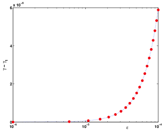
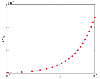
Figure 3: The numerical zeros of the determinant of the linear system (dots) and its best power fit (dashed line) for $\gamma_{1}=4$ (left) and $\gamma_{3}=24$ (right).

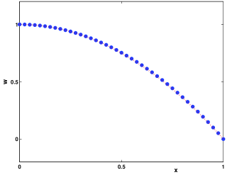
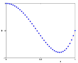
Figure 4: The numerical approximation of even eigenfunctions (dots) for $\varepsilon=10^{-4}$ near $\gamma_{1}=4$ (left) and $\gamma_{3}=24$ (right) and the even polynomial solutions for $\varepsilon=0$ (dashed line).

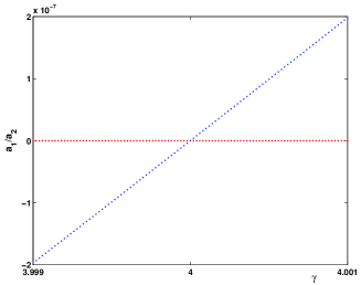
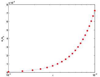
Figure 5: The ratio $a_{1}/a_{2}$ for the two equations in the linear system versus $\gamma$ for $\varepsilon=10^{-6}$ near $\gamma=\gamma_{1}=4$ (left) and for the solution of the linear system versus $\varepsilon$ (right). The best power fit is shown by dashed line.

Appendix A Appendix

A.1 Proof of Lemma 2.1.

Let us denote by $\lambda_{1}(L_{-}^{\varepsilon})$ the smallest eigenvalue of $L_{-}^{\varepsilon}$. We first show that $\lambda_{1}(L_{-}^{\varepsilon})\gtrsim 1$. Let $\chi\in C_{c}^{\infty}(\mathbb{R})$ be such that $0\leqslant\chi\leqslant 1$, ${\rm supp}(\chi)\subset(-3,3)$, and $\chi\equiv 1$ on $(-2,2)$. Let $\delta>0$ to be fixed later (independently of $\varepsilon$). The Max-Min principle ensures that

$$\lambda_{1}(L_{-}^{\varepsilon}) = \underset{v\in D(L_{-}^{\varepsilon})}{\inf}\frac{<L_{-}^{\varepsilon}v,v>}{\|v\|_{L^{2}}^{2}}$$ (A.1)

$$= \underset{v\in Q(L_{-}^{\varepsilon}),\|v\|_{L^{2}}=1}{\inf}\left(\|v^{\prime}\|_{L^{2}}^{2}+\int_{|x|>1}p_{\varepsilon}|v|^{2}dx\right)=\min\{\Lambda^{(1)},\Lambda^{(2)}\},$$

where

$$\Lambda^{(1)} = \underset{\text{\scriptsize$\begin{array}[]{c}v\in Q(L_{-}^{\varepsilon}),\|v\|_{L^{2}}=1,\\ \int_{|x|>2}|v|^{2}dx\geqslant\delta\end{array}$}}{\inf}\left(\|v^{\prime}\|_{L^{2}}^{2}+\int_{|x|>1}p_{\varepsilon}|v|^{2}dx\right),$$ (A.4)

$$\Lambda^{(2)} = \underset{\text{\scriptsize$\begin{array}[]{c}v\in Q(L_{-}^{\varepsilon}),\|v\|_{L^{2}}=1,\\ \int_{|x|>2}|v|^{2}dx\leqslant\delta\end{array}$}}{\inf}\left(\|v^{\prime}\|_{L^{2}}^{2}+\int_{|x|>1}p_{\varepsilon}|v|^{2}dx\right).$$ (A.7)

If $\|v\|_{L^{2}}=1$ and $\int_{|x|>2}|v|^{2}dx\geqslant\delta$, then

$$\int_{|x|>2}(x^{2}-1)|v|^{2}dx\geqslant 3\int_{|x|>2}|v|^{2}dx\geqslant 3\delta.$$

Therefore for $\varepsilon\leqslant 1$,

$$\Lambda^{(1)}\geqslant\frac{3\delta}{\varepsilon^{2}}\geqslant 3\delta.$$ (A.8)

On the other side, let us now take $v\in Q(L_{-}^{\varepsilon})$ such that $\|v\|_{L^{2}}=1$ and $\int_{|x|>2}|v|^{2}dx\leqslant\delta$. Then

$$\int_{|x|>1}(x^{2}-1)|\chi v|^{2}dx\leqslant\int_{|x|>1}(x^{2}-1)|v|^{2}dx,$$ (A.9)

and since $\chi^{\prime}(x)$ is supported in $\{2\leqslant|x|\leqslant 3\}$, we also have in this case

$$\int_{\mathbb{R}}|(\chi v)^{\prime}|^{2}dx = \int\left[\chi^{2}|v^{\prime}|^{2}+2\chi\chi^{\prime}vv^{\prime}+{\chi^{\prime}}^{2}|v|^{2}\right]dx$$ (A.10)

$$\leqslant \|v^{\prime}\|_{L^{2}(\mathbb{R})}^{2}+2\|v^{\prime}\|_{L^{2}(\mathbb{R})}\|\chi^{\prime}\|_{L^{\infty}(\mathbb{R})}\|v\|_{L^{2}(|x|>2)}+\|\chi^{\prime}\|_{L^{\infty}(\mathbb{R})}^{2}\|v\|_{L^{2}(|x|>2)}^{2}$$

$$\leqslant 2\|v^{\prime}\|_{L^{2}(\mathbb{R})}^{2}+2\delta\|\chi^{\prime}\|_{L^{\infty}(\mathbb{R})}^{2}.$$

Next, since $\chi\equiv 1$ on $\{|x|\leqslant 2\}$,

$$\int_{\mathbb{R}}|\chi v|^{2}dx\geqslant\int_{-2}^{2}|v|^{2}dx\geqslant 1-\delta.$$ (A.11)

Thanks to (A.9), (A.10) and (A.11), it turns out that

$$\frac{\int_{\mathbb{R}}|(\chi v)^{\prime}|^{2}dx+\int_{|x|>1}p_{\varepsilon}|\chi v|^{2}dx}{\int_{\mathbb{R}}|\chi v|^{2}dx}$$ (A.12)

$$\leqslant \frac{2\|v^{\prime}\|_{L^{2}(\mathbb{R})}^{2}+2\delta\|\chi^{\prime}\|_{L^{\infty}(\mathbb{R})}^{2}+\int_{|x|>1}p_{\varepsilon}|v|^{2}dx}{1-\delta}.$$

As a result, using (A.12), since $(\chi v)_{|(-3,3)}\in H_{0}^{1}(-3,3)$ for $v\in H^{1}(\mathbb{R})$,

$$\frac{2}{1-\delta}\Lambda^{(2)} \geqslant -\frac{2\delta\|\chi^{\prime}\|_{L^{\infty}(\mathbb{R})}^{2}}{1-\delta}+\underset{w\in H_{0}^{1}(-3,3)}{\inf}\frac{\int_{-3}^{3}|w^{\prime}|^{2}dx+\int_{|x|>1}p_{\varepsilon}|w|^{2}dx}{\int_{-3}^{3}|w|^{2}dx}$$ (A.13)

$$\geqslant -\frac{2\delta\|\chi^{\prime}\|_{L^{\infty}(\mathbb{R})}^{2}}{1-\delta}+\underset{w\in H_{0}^{1}(-3,3)}{\inf}\frac{\|w^{\prime}\|_{L^{2}}^{2}}{\|w\|_{L^{2}}^{2}}=:R_{\delta}.$$

Thanks to the Poincaré inequality, we can now choose $\delta\in(0,1)$ sufficiently small such that $R_{\delta}>0$. Then, according to (A.1), (A.8) and (A.13),

$$\lambda_{1}(L_{-}^{\varepsilon}) \geqslant \min\left(3\delta,\frac{(1-\delta)R_{\delta}}{2}\right),$$ (A.14)

which provides the estimate $\lambda_{1}(L_{-}^{\varepsilon})\gtrsim 1$ for $0<\varepsilon\leqslant 1$. The other estimate $\lambda_{1}(L_{-}^{\varepsilon})\lesssim 1$ is a direct consequence of (A.1) and of the Poincaré inequality. Indeed, the right hand side in (A.1) is bounded from above by the infimum of the same quantity, taken over $v\in L^{2}(\mathbb{R})$ such that $v_{|(-1,1)}\in H_{0}^{1}(-1,1)$ and $v_{|\{|x|>1\}}\equiv 0$. $\blacksquare$

A.2 Proof of Lemma 2.3.

To prove Lemma 2.3, we use the following lemma.

Lemma A.1

For $\varepsilon>0$,

$$L^{\varepsilon}:=-\partial_{x}^{2}+\frac{|x|}{\varepsilon^{2}}$$

defines a self-adjoint operator on $L^{2}(\mathbb{R})$. The spectrum of $L^{\varepsilon}$ is made of a sequence of strictly positive eigenvalues increasing to infinity, and the smallest eigenvalue satisfies

$$\lambda_{1}(L^{\varepsilon})\approx\varepsilon^{-4/3}.$$

• Proof. The first assertion is straightforward. Thanks to the Max-Min principle, $\lambda_{1}(L^{\varepsilon})$ is given by

  $$\lambda_{1}(L^{\varepsilon})=\underset{\text{\scriptsize$\begin{array}[]{c}v\in Q(L^{\varepsilon})\\ \|v\|_{L^{2}}=1\end{array}$}}{\inf}\left(\|v^{\prime}\|_{L^{2}}^{2}+\frac{1}{\varepsilon^{2}}\int_{\mathbb{R}}|x|v^{2}dx\right),$$

  where

  $$Q(L^{\varepsilon})=\{v\in H^{1}(\mathbb{R}):\;|x|^{1/2}v\in L^{2}(\mathbb{R})\}$$

  is the form domain of $L^{\varepsilon}$. If $v\in L^{2}(\mathbb{R})$ and $\|v\|_{L^{2}}=1$, $v$ can be rewritten as $v(x)=hw(h^{2}x)$, with $h>0$ and $w\in Q(L^{\varepsilon})$, with $\|w\|_{L^{2}}=1$ and $\|w^{\prime}\|_{L^{2}}=1$. Moreover, $h$ and $w$ are uniquely defined this way, and we have

  $$\|v^{\prime}\|_{L^{2}}^{2}=h^{4}$$

  and

  $$\int_{\mathbb{R}}|x|v^{2}dx=h^{-2}\int_{\mathbb{R}}|x|w^{2}dx.$$

  Thus,

  $$\lambda_{1}(L^{\varepsilon})=\underset{h>0}{\inf}\left(h^{4}+\varepsilon^{-2}h^{-2}\beta\right)=\left(\frac{1}{2^{2/3}}+2^{1/3}\right)\beta^{2/3}\varepsilon^{-4/3},$$

  where

  $$\beta:=\underset{\text{\scriptsize$\begin{array}[]{c}w\in Q(L^{\varepsilon})\\ \|w\|_{L^{2}}=1,\|w^{\prime}\|_{L^{2}}=1\end{array}$}}{\inf}\int_{\mathbb{R}}|x|w^{2}dx.$$

  The lemma follows if we prove that $\beta>0$. Let us assume by contradiction that $\beta=0$. Let $\left(w_{\delta}\right)_{\delta>0}$ be a minimizing sequence, that is $\|w_{\delta}\|_{L^{2}}=\|w_{\delta}^{\prime}\|_{L^{2}}=1$ and $\int_{\mathbb{R}}|x|w_{\delta}^{2}dx\to 0$ as $\delta\to 0$. Let $\chi\in\mathcal{C}_{c}^{\infty}(\mathbb{R})$ be such that $0\leqslant\chi\leqslant 1$, $\text{supp}(\chi)\subset[-1,1]$, and $\chi\equiv 1$ on $[-1/2,1/2]$. For $a>0$, we also define $\chi_{a}(x)=\chi(x/a)$, as well as $w_{\delta,a}:=\chi_{a}w_{\delta}$. Thanks to the Poincaré inequality, $\alpha:=\underset{v\in H_{0}^{1}(-1,1)}{\inf}\frac{\|v^{\prime}\|_{L^{2}}}{\|v\|_{L^{2}}}>0$, and then $\underset{v\in H_{0}^{1}(-a,a)}{\inf}\frac{\|v^{\prime}\|_{L^{2}}}{\|v\|_{L^{2}}}=\frac{\alpha}{a}>0$. Thus,

  $$\|w_{\delta,a}^{\prime}\|_{L^{2}(\mathbb{R})}^{2} \geqslant \frac{\alpha^{2}}{a^{2}}\|w_{\delta,a}\|_{L^{2}(\mathbb{R})}^{2}$$ (A.15)

  $$\geqslant \frac{\alpha^{2}}{a^{2}}\|w_{\delta}\|_{L^{2}(-\frac{a}{2},\frac{a}{2})}^{2}$$

  $$= \frac{\alpha^{2}}{a^{2}}\left(\|w_{\delta}\|_{L^{2}(\mathbb{R})}^{2}-\|w_{\delta}\|_{L^{2}(|x|>\frac{a}{2})}^{2}\right)$$

  $$\geqslant \frac{\alpha^{2}}{a^{2}}\left(1-\frac{2}{a}\int_{\mathbb{R}}|x|w_{\delta}^{2}dx\right).$$

  On the other side, since $\chi^{\prime}(x)$ is supported in $\left\{\frac{1}{2}\leqslant|x|\leqslant 1\right\}$, we have

  $$\|w_{\delta,a}^{\prime}\|_{L^{2}}^{2} = \int_{\mathbb{R}}\left((\chi^{\prime}_{a})^{2}w_{\delta}^{2}+2\chi_{a}\chi^{\prime}_{a}w_{\delta}w_{\delta}^{\prime}+\chi^{2}_{a}(w_{\delta}^{\prime})^{2}\right)dx$$

  $$\leqslant \frac{\|\chi^{\prime}\|_{L^{\infty}(\mathbb{R})}^{2}}{a^{2}}\|w_{\delta}\|^{2}_{L^{2}(\frac{a}{2}<|x|<a)}+\frac{2}{a}\|\chi^{\prime}\|_{L^{\infty}(\mathbb{R})}\|w_{\delta}\|_{L^{2}(\frac{a}{2}<|x|<a)}\|w_{\delta}^{\prime}\|_{L^{2}(\mathbb{R})}+\|w_{\delta}^{\prime}\|_{L^{2}(\mathbb{R})}^{2}.$$

  According to the assumption, given $a>0$, we can find $\delta(a)$ sufficiently small such that

  $$\int_{\mathbb{R}}|x|w_{\delta(a)}^{2}dx\leqslant a^{2}.$$

  Then,

  $$\int_{\frac{a}{2}<|x|<a}w_{\delta}^{2}dx\leqslant\int_{|x|>\frac{a}{2}}w_{\delta}^{2}dx\leqslant\frac{2}{a}\int_{\mathbb{R}}|x|w_{\delta}^{2}dx\leqslant 2a.$$ (A.17)

  It follows from (A.15), ( ‣ A.2) and (A.17) with $\delta=\delta(a)$ that

  $$\frac{\alpha^{2}}{a^{2}}(1-2a)\leqslant\frac{2\|\chi^{\prime}\|_{L^{\infty}(\mathbb{R})}^{2}}{a}+\frac{2^{3/2}\|\chi^{\prime}\|_{L^{\infty}(\mathbb{R})}}{a^{1/2}}+1.$$

  Letting $a$ go to $0$ yields to a contradiction, which completes the proof of the lemma.  

Thanks to the Max-Min principle, we know that the lowest eigenvalue of $L_{+}^{\varepsilon}$ is given by

$$\lambda_{1}(L_{+}^{\varepsilon}) = \underset{v\in Q(L_{+}^{\varepsilon})}{\inf}\frac{\|v^{\prime}\|_{L^{2}}^{2}+\int_{\mathbb{R}}q_{\varepsilon}|v|^{2}dx}{\|v\|_{L^{2}}^{2}},$$ (A.18)

where

$$Q(L_{+}^{\varepsilon})=\{v\in H^{1}(\mathbb{R}):\;xv\in L^{2}(\mathbb{R})\}$$

is the form domain of $L_{+}^{\varepsilon}$. The statement of Lemma 2.3 is equivalent to $\lambda_{1}(L_{+}^{\varepsilon})\approx\varepsilon^{-4/3}$. We first prove the upper bound on $\lambda_{1}(L_{+}^{\varepsilon})$. Let us define $v_{\varepsilon}$ on $\mathbb{R}$ as

$$v_{\varepsilon}(x):=\left\{\begin{array}[]{ll}x-1+\varepsilon^{2/3}&\text{for}\;\;1-\varepsilon^{2/3}<x<1,\\ -(x-1-\varepsilon^{2/3})&\text{for}\;\;1<x<1+\varepsilon^{2/3},\\ 0&\text{elsewhere}.\end{array}\right.$$

and denote $q(x):=\varepsilon^{2}q_{\varepsilon}(x)=2(1-x^{2})\mathbf{1}_{\{|x|<1\}}+(x^{2}-1)\mathbf{1}_{\{|x|>1\}}$. Then

$$\|v_{\varepsilon}^{\prime}\|_{L^{2}(\mathbb{R})}^{2}=2\varepsilon^{2/3},\quad\|v_{\varepsilon}\|_{L^{2}(\mathbb{R})}^{2}=\frac{2\varepsilon^{2}}{3},$$

and since $q(x)\leqslant 4|x-1|$ for $|x-1|\leqslant 1$,

$$\int_{\mathbb{R}}q_{\varepsilon}|v_{\varepsilon}|^{2}dx\leqslant\frac{4}{\varepsilon^{2}}\int_{1-\varepsilon^{2/3}}^{1+\varepsilon^{2/3}}|1-x|v_{\varepsilon}^{2}dx=\frac{2\varepsilon^{2/3}}{3}.$$

As a result,

$$\lambda_{1}(L_{+}^{\varepsilon})\leqslant\frac{2\varepsilon^{2/3}+2\varepsilon^{2/3}/3}{2\varepsilon^{2}/3}=4\varepsilon^{-4/3}.$$

It remains to find a bound on $\lambda_{1}(L_{+}^{\varepsilon})$ from below. Let us first introduce the two intervals

$$D_{+}:=\left\{x\geqslant 0,\;\;q(x)\leqslant\frac{1}{2}\right\}=\left[\frac{\sqrt{3}}{2},\sqrt{\frac{3}{2}}\right],\quad D_{-}:=\left\{x\leqslant 0,\;\;q(x)\leqslant\frac{1}{2}\right\}=-D_{+},$$

and denote $D:=D_{+}\cup D_{-}$. If $v\in Q(L_{+}^{\varepsilon})$, $\|v\|_{L^{2}}=1$ and $\int_{D}|v|^{2}dx\leqslant 1-\varepsilon^{1/2}$, then

$$\int_{\mathbb{R}}q|v|^{2}dx\geqslant\int_{\mathbb{R}\D}q|v|^{2}dx\geqslant\frac{1}{2}\int_{\mathbb{R}\D}|v|^{2}dx\geqslant\frac{\varepsilon^{1/2}}{2}>4\varepsilon^{2/3}$$

for sufficiently small $\varepsilon>0$. As a result, thanks to (A.18) and the upper bound on $\lambda_{1}(L_{+}^{\varepsilon})$, we deduce that

$$\lambda_{1}(L_{+}^{\varepsilon}) = \underset{\text{\scriptsize$\begin{array}[]{c}v\in Q(L_{+}^{\varepsilon}),\\ \|v\|_{L^{2}}=1,\\ \int_{D}|v|^{2}dx\geqslant 1-\varepsilon^{1/2}\end{array}$}}{\inf}\left[\|v^{\prime}\|_{L^{2}}^{2}+\int_{\mathbb{R}}q_{\varepsilon}|v|^{2}dx\right].$$ (A.22)

From now on, we assume that $v\in Q(L_{+}^{\varepsilon})$, $\|v\|_{L^{2}}=1$ and $\int_{D}|v|^{2}dx\geqslant 1-\varepsilon^{1/2}$. Let $\chi\in\mathcal{C}_{c}^{\infty}(\mathbb{R})$ be such that $0\leqslant\chi\leqslant 1$, ${\rm supp}(\chi)\subset[-1/2,1/2]\subset\mathbb{R}\D$, and $\chi(x)\equiv 1$ for $x\in[-1/4,1/4]$. We also define $\rho:=1-\chi$. In particular, $\rho\equiv 1$ on $D$, thus

$$\|\rho v\|_{L^{2}}^{2}\geqslant\int_{D}|v|^{2}dx\geqslant 1-\varepsilon^{1/2},\quad\int_{\mathbb{R}}q|\rho v|^{2}dx\leqslant\int_{\mathbb{R}}q|v|^{2}dx,$$ (A.23)

and since $\rho^{\prime}$ is supported in $\mathbb{R}\D$, for some $C>0$, we have

$$\int_{\mathbb{R}}|(\rho v)^{\prime}|^{2}dx \leqslant \|\rho^{\prime}\|_{L^{\infty}(\mathbb{R})}^{2}\|v\|^{2}_{L^{2}(\mathbb{R}\D)}+\|v^{\prime}\|_{L^{2}(\mathbb{R})}^{2}+2\|\rho\|_{L^{\infty}(\mathbb{R})}\|\rho^{\prime}\|_{L^{\infty}(\mathbb{R})}\|v^{\prime}\|_{L^{2}(\mathbb{R})}\|v\|_{L^{2}(\mathbb{R}\D)}$$ (A.24)

$$\leqslant C\varepsilon^{1/2}+\|v^{\prime}\|_{L^{2}(\mathbb{R})}^{2}+C\varepsilon^{1/4}\|v^{\prime}\|_{L^{2}(\mathbb{R})}$$

$$\leqslant 2(\|v^{\prime}\|_{L^{2}(\mathbb{R})}^{2}+C\varepsilon^{1/2}).$$

Therefore, combining (A.23) and (A.24), we obtain, for $\varepsilon$ sufficiently small,

$$\frac{\|(\rho v)^{\prime}\|_{L^{2}}^{2}+\int_{\mathbb{R}}q_{\varepsilon}|\rho v|^{2}dx}{\|\rho v\|_{L^{2}}^{2}} \leqslant \frac{2(\|v^{\prime}\|_{L^{2}(\mathbb{R})}^{2}+C\varepsilon^{1/2})+\int_{\mathbb{R}}q_{\varepsilon}|v|^{2}dx}{1-\varepsilon^{1/2}}$$ (A.25)

$$\leqslant 2(\|v^{\prime}\|_{L^{2}}^{2}+\int_{\mathbb{R}}q_{\varepsilon}|v|^{2}dx)+2C\varepsilon^{1/2}.$$

Taking the infimum in $v$ in (A.25), we infer thanks to (A.22) that

$$2\lambda_{1}(L_{+}^{\varepsilon})+2C\varepsilon^{1/2} \geqslant \underset{\text{\scriptsize$\begin{array}[]{c}v\in Q(L_{+}^{\varepsilon}),\\ \|v\|_{L^{2}}=1,\\ \int_{D}|v|^{2}dx\geqslant 1-\varepsilon^{1/2}\end{array}$}}{\inf}\frac{\|(\rho v)^{\prime}\|_{L^{2}}^{2}+\int_{\mathbb{R}}q_{\varepsilon}|\rho v|^{2}dx}{\|\rho v\|_{L^{2}}^{2}}.$$ (A.29)

Therefore, since $q(x)\geqslant 2|x-1|$ for $x\geqslant 0$ and $q(x)\geqslant 2|x+1|$ for $x\leqslant 0$, and decomposing $\rho v=v_{1}+v_{2}$ with $v_{1}$ supported in $(-\infty,-1/4]$ and $v_{2}$ supported in $[1/4,+\infty)$, we have

$$2\lambda_{1}(L_{+}^{\varepsilon})+2C\varepsilon^{1/2}$$ (A.33)

$$\geqslant \!\!\!\!\!\underset{\text{\scriptsize$\begin{array}[]{c}v_{1},v_{2}\in Q(L_{+}^{\varepsilon}),\\ \text{supp}(v_{1})\subset(-\infty,-1/4],\\ \text{supp}(v_{2})\subset[1/4,+\infty)\end{array}$}}{\inf}\frac{\|v_{1}^{\prime}\|_{L^{2}}^{2}+\int_{\mathbb{R}}q_{\varepsilon}|v_{1}|^{2}dx+\|v_{2}^{\prime}\|_{L^{2}}^{2}+\int_{\mathbb{R}}q_{\varepsilon}|v_{2}|^{2}dx}{\|v_{1}\|_{L^{2}}^{2}+\|v_{2}\|_{L^{2}}^{2}}$$

$$\geqslant \!\!\!\!\!\underset{\text{\scriptsize$\begin{array}[]{c}v_{1},v_{2}\in Q(L_{+}^{\varepsilon}),\\ \text{supp}(v_{1})\subset(-\infty,-1/4],\\ \text{supp}(v_{2})\subset[1/4,+\infty)\end{array}$}}{\inf}\frac{\|v_{1}^{\prime}\|_{L^{2}}^{2}+\frac{2}{\varepsilon^{2}}\int_{\mathbb{R}}|x+1||v_{1}|^{2}dx+\|v_{2}^{\prime}\|_{L^{2}}^{2}+\frac{2}{\varepsilon^{2}}\int_{\mathbb{R}}|x-1||v_{2}|^{2}dx}{\|v_{1}\|_{L^{2}}^{2}+\|v_{2}\|_{L^{2}}^{2}}$$ (A.37)

$$\geqslant \underset{\text{\scriptsize$\begin{array}[]{c}v_{1},v_{2}\in Q(L_{+}^{\varepsilon})\end{array}$}}{\inf}\frac{\|v_{1}^{\prime}\|_{L^{2}}^{2}+\frac{2}{\varepsilon^{2}}\int_{\mathbb{R}}|x+1||v_{1}|^{2}dx+\|v_{2}^{\prime}\|_{L^{2}}^{2}+\frac{2}{\varepsilon^{2}}\int_{\mathbb{R}}|x-1||v_{2}|^{2}dx}{\|v_{1}\|_{L^{2}}^{2}+\|v_{2}\|_{L^{2}}^{2}}$$ (A.39)

$$= \underset{\text{\scriptsize$\begin{array}[]{c}v_{1},v_{2}\in Q(L_{+}^{\varepsilon})\end{array}$}}{\inf}\frac{\|v_{1}^{\prime}\|_{L^{2}}^{2}+\frac{2}{\varepsilon^{2}}\int_{\mathbb{R}}|x||v_{1}|^{2}dx+\|v_{2}^{\prime}\|_{L^{2}}^{2}+\frac{2}{\varepsilon^{2}}\int_{\mathbb{R}}|x||v_{2}|^{2}dx}{\|v_{1}\|_{L^{2}}^{2}+\|v_{2}\|_{L^{2}}^{2}}$$ (A.41)

$$= \underset{\text{\scriptsize$\begin{array}[]{c}v_{1},v_{2}\in Q(L_{+}^{\varepsilon})\\ \|v_{1}\|_{L^{2}}\leqslant\|v_{2}\|_{L^{2}}\end{array}$}}{\inf}\frac{\|v_{1}^{\prime}\|_{L^{2}}^{2}+\frac{2}{\varepsilon^{2}}\int_{\mathbb{R}}|x||v_{1}|^{2}dx+\|v_{2}^{\prime}\|_{L^{2}}^{2}+\frac{2}{\varepsilon^{2}}\int_{\mathbb{R}}|x||v_{2}|^{2}dx}{\|v_{1}\|_{L^{2}}^{2}+\|v_{2}\|_{L^{2}}^{2}}$$ (A.44)

$$\geqslant \underset{\text{\scriptsize$\begin{array}[]{c}v_{1},v_{2}\in Q(L_{+}^{\varepsilon})\\ \|v_{1}\|_{L^{2}}\leqslant\|v_{2}\|_{L^{2}}=1\end{array}$}}{\inf}\left(\frac{\|v_{1}^{\prime}\|_{L^{2}}^{2}+\frac{2}{\varepsilon^{2}}\int_{\mathbb{R}}|x||v_{1}|^{2}dx}{2}+\frac{\|v_{2}^{\prime}\|_{L^{2}}^{2}+\frac{2}{\varepsilon^{2}}\int_{\mathbb{R}}|x||v_{2}|^{2}dx}{2}\right)$$ (A.47)

$$\geqslant \frac{1}{2}\underset{\text{\scriptsize$\begin{array}[]{c}v_{2}\in Q(L_{+}^{\varepsilon})\\ \|v_{2}\|_{L^{2}}=1\end{array}$}}{\inf}\left(\|v_{2}^{\prime}\|_{L^{2}}^{2}+\frac{2}{\varepsilon^{2}}\int_{\mathbb{R}}|x||v_{2}|^{2}dx\right)\geqslant\frac{1}{2}\lambda_{1}(L^{\varepsilon})\gtrsim\varepsilon^{-4/3},$$ (A.50)

where we have used Lemma A.1 in the last estimation. $\blacksquare$

A.3 Proofs of Lemmas 2.6 and 4.1

Proof of Lemma 2.6.  

The proof of Lemma 2.6 relies on WKB approximation techniques, explained for instance in [M]. If we define $w(x):=\psi(1-x)$, it is equivalent for $\psi$ to solve (2.37) or for $w$ to solve

$$\varepsilon^{2}w^{\prime\prime}-2x(2-x)w=0,\quad x\in\left(0,\frac{3}{2}\right).$$ (A.51)

In the new variable $\xi=\xi(x):=\left(\frac{3}{2}\int_{0}^{x}\sqrt{2t(2-t)}dt\right)^{2/3}$, it is equivalent for $w$ to solve (A.51) or for $v(\xi):=\frac{w(x)}{a(x)}$ to solve

$$\varepsilon^{2}\frac{d^{2}v}{d\xi^{2}}-\xi v=\varepsilon^{2}\delta(\xi)v,\quad\xi\in(0,\xi_{0}),$$ (A.52)

where $\xi_{0}:=\xi(3/2)$, $a(x):=\left(\xi^{\prime}(x)\right)^{-1/2}$, and $\delta(\xi):=-a^{\prime\prime}(x)a^{3}(x)$. Next, we look for $v$ in the form $v(\xi)={\rm Ai}\left(\frac{\xi}{\varepsilon^{2/3}}\right)(1+Q(\xi))$. Using that ${\rm Ai}(\xi/\varepsilon^{2/3})$ solves the homogeneous equation

$$\varepsilon^{2}\frac{d^{2}v}{d\xi^{2}}-\xi v=0,$$

it is equivalent for $v$ to solve (A.52) or for $Q$ to solve

$$\frac{d}{d\xi}\left[{\rm Ai}\left(\frac{\xi}{\varepsilon^{2/3}}\right)^{2}Q^{\prime}(\xi)\right] = \delta(\xi){\rm Ai}\left(\frac{\xi}{\varepsilon^{2/3}}\right)^{2}(1+Q(\xi)),\quad\xi\in(0,\xi_{0}).$$ (A.53)

By integration, (A.53) is equivalent to the integral equation

$$Q(\xi)=F(Q)(\xi):=\int_{\xi}^{\xi_{0}}\int_{\xi}^{\eta}\frac{{\rm Ai}\left(\frac{\eta}{\varepsilon^{2/3}}\right)^{2}}{{\rm Ai}\left(\frac{t}{\varepsilon^{2/3}}\right)^{2}}dt\delta(\eta)(1+Q(\eta))d\eta,$$ (A.54)

where $F$ maps $\mathcal{C}^{0}([0,\xi_{0}])$ into itself. A change of variable provides

$$F(Q)(\xi)=\varepsilon^{2/3}\int_{\xi}^{\xi_{0}}\left(\int_{\xi/\varepsilon^{2/3}}^{\eta/\varepsilon^{2/3}}{\rm Ai}(u)^{-2}du{\rm Ai}\left(\frac{\eta}{\varepsilon^{2/3}}\right)^{2}\right)\delta(\eta)(1+Q(\eta))d\eta.$$

Thanks to the asymptotic behavior (2.38), $f(x):=\int_{0}^{x}{\rm Ai}(y)^{-2}dy{\rm Ai}(x)^{2}\sim\frac{1}{2\sqrt{x}}$ as $x\to+\infty$. In particular, $f$ is bounded on $\mathbb{R}_{+}$. We deduce that for any $\xi\in(0,\xi_{0})$,

$$\left|(F(Q))(\xi)\right|\leqslant\varepsilon^{2/3}\|f\|_{L^{\infty}(\mathbb{R}_{+})}\int_{\xi}^{\xi_{0}}|\delta(\eta)|d\eta(1+\|Q\|_{L^{\infty}(0,\xi_{0})}).$$

Since $\delta$ is clearly continuous on $(0,\xi_{0}]$ and

$$\delta(\xi(x))\longrightarrow\frac{9\cdot 2^{2/3}}{560}\quad\mbox{as}\quad x\to 0,$$

we deduce $\delta\in L^{1}(0,\xi_{0})$. Thus, if $Q\in\mathcal{C}^{0}([0,\xi_{0}])$, then

$$\|F(Q)\|_{L^{\infty}(0,\xi_{0})}\leqslant\varepsilon^{2/3}\|f\|_{L^{\infty}(\mathbb{R}_{+})}\|\delta\|_{L^{1}(0,\xi_{0})}(1+\|Q\|_{L^{\infty}(0,\xi_{0})}).$$ (A.55)

Moreover, if $Q_{1},Q_{2}\in\mathcal{C}^{0}([0,\xi_{0}])$, we get similarly

$$\|F(Q_{1})-F(Q_{2})\|_{L^{\infty}(0,\xi_{0})}\leqslant\varepsilon^{2/3}\|f\|_{L^{\infty}(\mathbb{R}_{+})}\|\delta\|_{L^{1}(0,\xi_{0})}\|Q_{1}-Q_{2}\|_{L^{\infty}(0,\xi_{0})}.$$ (A.56)

From (A.55) and (A.56) we infer that, if we take $C:=2\|f\|_{L^{\infty}(\mathbb{R}_{+})}\|\delta\|_{L^{1}(0,\xi_{0})}$, for $\varepsilon$ sufficiently small (namely $\varepsilon^{2/3}<1/2C$), $F$ maps the ball of radius $C\varepsilon^{2/3}$ in $\mathcal{C}^{0}([0,\xi_{0}])$ into itself, and is a contraction on that ball. Then, $F$ has a unique fixed point $Q$ such that $\|Q\|_{L^{\infty}(0,\xi_{0})}\leqslant C\varepsilon^{2/3}$. Such a fixed point of $F$ gives a $\mathcal{C}^{2}$ solution of (A.53) on $(0,\xi_{0})$. Defining $Q_{A}^{\varepsilon}$ as $Q_{A}^{\varepsilon}(x):=Q(\xi(1-x))$ and applying the sequence of substitutions backwards, we found a solution $\psi_{A}^{\varepsilon}$ of the system (2.37) with the required bounds.

For the existence of the solution $\psi_{B}^{\varepsilon}$, we proceed similarly. Namely, we look for a solution to (A.52) in the form $v(\xi)={\rm Bi}\left(\frac{\xi}{\varepsilon^{2/3}}\right)(1+Q(\xi))$. It is equivalent for $v$ to solve (A.52) or for $Q$ to solve

$$\frac{d}{d\xi}\left[{\rm Bi}\left(\frac{\xi}{\varepsilon^{2/3}}\right)^{2}Q^{\prime}(\xi)\right] = \delta(\xi){\rm Bi}\left(\frac{\xi}{\varepsilon^{2/3}}\right)^{2}(1+Q(\xi)),\quad\xi\in(0,\xi_{0}).$$ (A.57)

Since $g(x):={\rm Bi}(x)^{2}\int_{x}^{+\infty}{\rm Bi}(u)^{-2}du\sim\frac{1}{2\sqrt{x}}$ as $x\to+\infty$ thanks to the asymptotic behavior (2.38) again, $g$ is bounded on $\mathbb{R}_{+}$. It enables us to prove the existence of a fixed point to the functional $G:\mathcal{C}^{0}([0,\xi_{0}])\mapsto\mathcal{C}^{0}([0,\xi_{0}])$ defined by

$$G(Q)(\xi):=\int_{0}^{\xi}\int_{\eta}^{\xi}\frac{{\rm Bi}\left(\frac{\eta}{\varepsilon^{2/3}}\right)^{2}}{{\rm Bi}\left(\frac{t}{\varepsilon^{2/3}}\right)^{2}}dt\delta(\eta)(1+Q(\eta))d\eta,$$

similarly to what has been done for $F$.

The linear independence of $\psi_{A}^{\varepsilon}$ and $\psi_{B}^{\varepsilon}$ follows from the linear independence of functions ${\rm Ai}$ and ${\rm Bi}$. $\blacksquare$

Proof of Lemma 4.1.  

The proof is very similar to that of Lemma 2.6, so that we will only point out the differences. It is equivalent for $\psi$ to solve (4.7) on $(\sqrt{1+\varepsilon\nu},+\infty)$ or for $w(x):=\psi(\sqrt{1+\varepsilon\nu}(1+x))$ to solve

$$\tilde{\varepsilon}^{2}w^{\prime\prime}(x)-x(x+2)w(x)=0$$ (A.58)

on $\mathbb{R}^{+}$, where $\tilde{\varepsilon}:=\varepsilon/\sqrt{1+\varepsilon\nu}$. We look for $w$ in the form $w(x)=a(x)v(\xi(x))$, where $\xi(x)=\left(\frac{3}{2}\int_{0}^{x}\sqrt{t(2+t)}dt\right)^{2/3}$ and $a(x)=(\xi^{\prime}(x))^{-1/2}$. Then, it is equivalent for $w$ to solve (A.58) on $\mathbb{R}^{+}$ or for $v$ to solve

$$\tilde{\varepsilon}^{2}v^{\prime\prime}(\xi)-\xi v(\xi)=\tilde{\varepsilon}^{2}\delta(\xi)v(\xi)$$ (A.59)

on $\mathbb{R}^{+}$, where the function $\xi\mapsto\delta(\xi)$ is defined by $\delta(\xi(x))=-a^{\prime\prime}(x)a(x)^{3}$. Since $a\in\mathcal{C}^{\infty}([0,+\infty))$ and $\delta(\xi)\underset{\xi\to\infty}{\sim}7\xi^{-2}/1024$, we deduce that $\delta\in L^{1}(\mathbb{R}^{+})$. Then, the existence of $Q\in\mathcal{C}_{b}^{0}(\mathbb{R}^{+})$ with $\|Q\|_{L^{\infty}(\mathbb{R}^{+})}\lesssim\varepsilon^{2/3}$, such that $v(\xi)={\rm Ai}(\xi/\tilde{\varepsilon}^{2/3})(1+Q(\xi))$ solves (A.59), is established like in the proof of Lemma 2.6, applying the fixed point theorem to the functional $F$ defined in (A.54), with $\xi_{0}=+\infty$. Therefore, we obtain $\psi_{A}^{\nu,\varepsilon}$. The expression for $\psi_{B}^{\nu,\varepsilon}$ is obtained similarly as in Lemma 2.6. Next, the expression of $\psi_{A}^{\nu,\varepsilon}(x)$ at $x=\sqrt{1+\varepsilon\nu}$ yields

$$\psi_{A}^{\nu,\varepsilon}(\sqrt{1+\varepsilon\nu})=a(0){\rm Ai}(0)(1+Q_{A}^{\nu,\varepsilon}(0))=a(0){\rm Ai}(0)(1+\mathcal{O}(\varepsilon^{2/3})),$$ (A.60)

and similarly

$$(\psi_{A}^{\nu,\varepsilon})^{\prime}(\sqrt{1+\varepsilon\nu})$$ (A.61)

$$= a^{\prime}(0){\rm Ai}(0)(1+\mathcal{O}(\varepsilon^{2/3}))+a(0)\xi^{\prime}(0){\rm Ai}^{\prime}(0)\varepsilon^{-2/3}(1+\mathcal{O}(\varepsilon^{2/3}))+a(0){\rm Ai}(0)\xi^{\prime}(0)(Q_{A}^{\nu,\varepsilon})^{\prime}(0)$$

$$= a(0)\xi^{\prime}(0){\rm Ai}^{\prime}(0)\varepsilon^{-2/3}(1+\mathcal{O}(\varepsilon^{2/3})),$$

where we have used that

$$\left|(Q_{A}^{\nu,\varepsilon})^{\prime}(0)\right|=\left|{\rm Ai}(0)^{-2}\int_{0}^{+\infty}{\rm Ai}(\eta/\tilde{\varepsilon}^{2/3})^{2}\delta(\eta)(1+Q_{A}^{\nu,\varepsilon}(\eta))d\eta\right|\leqslant\|\delta\|_{L^{1}(\mathbb{R}^{+})}(1+{\cal O}(\varepsilon^{2/3}))\lesssim 1.$$

At this point, the function $\psi_{A}^{\nu,\varepsilon}$ has been defined on the interval $[\sqrt{1+\varepsilon\nu},+\infty)$. In the case $\nu>0$, we extend into a solution of (4.7) on the interval $[1,+\infty)$, thanks to the Cauchy-Lipshitz Theorem. We denote $I_{\nu}=[\sqrt{1+\varepsilon\nu},1]$ if $\nu<0$, $I_{\nu}=[1,\sqrt{1+\varepsilon\nu}]$ if $\nu>0$. Then, for any sign of $\nu$, we have

$$\left|\psi_{A}^{\nu,\varepsilon}(1)-\psi_{A}^{\nu,\varepsilon}(\sqrt{1+\varepsilon\nu})\right| \lesssim \varepsilon\|(\psi_{A}^{\nu,\varepsilon})^{\prime}\|_{L^{\infty}(I_{\nu})}\lesssim\varepsilon\left|(\psi_{A}^{\nu,\varepsilon})^{\prime}(\sqrt{1+\varepsilon\nu})\right|+\varepsilon^{2}\|(\psi_{A}^{\nu,\varepsilon})^{\prime\prime}\|_{L^{\infty}(I_{\nu})}$$ (A.62)

$$\lesssim \varepsilon^{1/3}+\varepsilon\|\psi_{A}^{\nu,\varepsilon}\|_{L^{\infty}(I_{\nu})}$$

and, thanks to (A.62)

$$\|\psi_{A}^{\nu,\varepsilon}\|_{L^{\infty}(I_{\nu})} \lesssim \left|\psi_{A}^{\nu,\varepsilon}(\sqrt{1+\varepsilon\nu})\right|+\varepsilon\|(\psi_{A}^{\nu,\varepsilon})^{\prime}\|_{L^{\infty}(I_{\nu})}$$

$$\lesssim 1+\varepsilon\|\psi_{A}^{\nu,\varepsilon}\|_{L^{\infty}(I_{\nu})},$$

thus

$$\|\psi_{A}^{\nu,\varepsilon}\|_{L^{\infty}(I_{\nu})} \lesssim 1.$$ (A.63)

From (A.62), (A.63) and (A.60) it follows that

$$\psi_{A}^{\nu,\varepsilon}(1)=a(0){\rm Ai}(0)(1+{\cal O}(\varepsilon^{1/3}).$$ (A.64)

Similarly,

$$\left|(\psi_{A}^{\nu,\varepsilon})^{\prime}(1)-(\psi_{A}^{\nu,\varepsilon})^{\prime}(\sqrt{1+\varepsilon\nu})\right| \lesssim \varepsilon\|(\psi_{A}^{\nu,\varepsilon})^{\prime\prime}\|_{L^{\infty}(I_{\nu})}\lesssim\|\psi_{A}^{\nu,\varepsilon}\|_{L^{\infty}(I_{\nu})}\lesssim 1,$$

and therefore thanks to (A.61), we get

$$(\psi_{A}^{\nu,\varepsilon})^{\prime}(1)=a(0)\xi^{\prime}(0){\rm Ai}^{\prime}(0)\varepsilon^{-2/3}(1+{\cal O}(\varepsilon^{2/3}).$$ (A.65)

The limit (4.8) follows from (A.64) and (A.65), since $\xi^{\prime}(0)=2^{1/3}$, and because

$${\rm Ai}(0)=\frac{1}{3^{2/3}\Gamma(2/3)},\quad{\rm Ai}^{\prime}(0)=-\frac{1}{3^{1/3}\Gamma(1/3)}.$$

Notice that all the estimates we made in this proof are uniform in $\nu\in K$, for any fixed compact subset $K\subset\mathbb{R}$. $\blacksquare$

A.4 Proof of Lemma 3.8

If $f\in X^{\prime}$ and $\varphi\in D(L_{X})$, we have

$$|\left<L_{X^{\prime}}f,\varphi\right>_{D(L_{X})^{\prime},D(L_{X})}|\leqslant\|f\|_{X^{\prime}}\|L_{X}\varphi\|_{X}\leqslant\|f\|_{X^{\prime}}\|\varphi\|_{D(L_{X})},$$

which provides the continuity of $L_{X}$. If $f\in X^{\prime}$ and $L_{X^{\prime}}f=0$, then for every $\varphi\in D(L_{X})$, $\left<f|L_{X}\varphi\right>_{X^{\prime},X}=0$. We can apply this to $\varphi=L_{X}^{-1}x$, for any $x\in X$ and we get that $\left<f,x\right>_{X^{\prime},X}=0$ for every $x\in X$. Therefore $f=0$ and $L_{X^{\prime}}$ is injective. Let us next prove the surjectivity of $L_{X^{\prime}}$. Let $T\in D(L_{X})^{\prime}$. $f:x\mapsto\left<T,L_{X}^{-1}x\right>_{D(L_{X})^{\prime},D(L_{X})}$ clearly defines a continuous linear form on $X$, and for every $\varphi\in D(L_{X})$,

$$\left<L_{X^{\prime}}f,\varphi\right>_{D(L_{X})^{\prime},D(L_{X})}=\left<f,L_{X}\varphi\right>_{X^{\prime},X}=\left<T,L_{X}^{-1}L_{X}\varphi\right>_{D(L_{X})^{\prime},D(L_{X})}=\left<T,\varphi\right>_{D(L_{X})^{\prime},D(L_{X})},$$

which means that $T=L_{X^{\prime}}f$. Moreover, the application $L_{X^{\prime}}^{-1}:D(L_{X})^{\prime}\mapsto X^{\prime}$ we have just defined is continuous. Indeed, if $T\in D(L_{X})^{\prime}$ and $x\in X$,

$$|\left<L_{X^{\prime}}^{-1}T,x\right>_{X^{\prime},X}| = |\left<T,L_{X}^{-1}x\right>_{D(L_{X})^{\prime},D(L_{X})}|$$

$$\leqslant \|T\|_{D(L_{X})^{\prime}}\|L_{X}^{-1}x\|_{D(L_{X})}$$

$$\lesssim \|T\|_{D(L_{X})^{\prime}}(\|x\|_{X}+\|L^{-1}x\|_{D(L)})$$

$$\lesssim \|T\|_{D(L_{X})^{\prime}}\|x\|_{X},$$

where we have used the continuous embeddings $D(L)\subset X\subset H$, as well as the continuity of $L^{-1}\in\mathcal{L}(H)$. Finally, we show that $L_{X^{\prime}}$ is an extension of $L$. Here, we classically identify elements of $H$ to elements of $X^{\prime}$ (resp. $D(L_{X})^{\prime}$) as follows: if $f\in H$, $x\in X$ (resp. $T\in H$, $\varphi\in D(L_{X})$), $\left<f,x\right>_{X^{\prime},X}=(f|\overline{x})$ (resp. $\left<T,\varphi\right>_{D(L_{X})^{\prime},D(L_{X})}=(T|\overline{\varphi})$), where $(\cdot|\cdot)$ denotes the scalar product in $H$. Thus, if $f\in D(L)\subset X\subset X^{\prime}$,

$$\left<L_{X^{\prime}}f,\varphi\right>_{D(L_{X})^{\prime},D(L_{X})}=\left<f,L\varphi\right>_{X^{\prime},X}=\left(f|\overline{L\varphi}\right)=\left(Lf|\overline{\varphi}\right)=\left<Lf,\varphi\right>_{D(L_{X})^{\prime},D(L_{X})},$$

which means that $L_{X^{\prime}}f=Lf$. $\blacksquare$

A.5 Numerical methods for inner solutions

We rewrite the fourth–order equation (4.3) on $[0,1]$ in the form

$$w^{\prime\prime}(x)=v(x),\quad\varepsilon^{2}v^{\prime\prime}(x)-2(1-x^{2})v(x)=\gamma w(x),\quad 0<x<1.$$

Using the finite-difference approximation with the second–order central differences [GP], the system of differential equations is converted into the system of algebraic equations

$$A_{1}{\bf w}={\bf v},\quad A_{2}{\bf v}=\gamma{\bf w},$$

where ${\bf v},{\bf w}$ are $n$-vectors of $v(x)$,$w(x)$ represented on a discrete grid $\{x_{k}\}_{k=0}^{n-1}\subset[0,1]$ with $x_{0}=0$ and $x_{0}<x_{1}<...<x_{n-1}<x_{n}=1$. Using an equally spaced grid with step size $h=1/n$ and incorporating boundary conditions $w^{\prime}(0)=0$, $v^{\prime}(0)=0$, we obtain $n\times n$ matrices $A_{1}$ and $A_{2}$ in the explicit form, where

$$A_{1}=\frac{1}{h^{2}}\left[\begin{array}[]{cccccc}-2&2&0&...&0&0\\ 1&-2&1&...&0&0\\ 0&1&-2&...&0&0\\ \vdots&\vdots&\vdots&\vdots&\vdots&\vdots\\ 0&0&0&...&1&-2\end{array}\right]$$

and $A_{2}=\varepsilon^{2}A_{1}-2{\rm diag}(1-x^{2})$. For the first solution $w_{1}(x)$, with $w_{n}=1$ and $v_{n}=0$, we obtain solutions of the finite-difference equations in the form

$${\bf w}=-\frac{1}{h^{2}}\left(A_{1}-\gamma A_{2}^{-1}\right)^{-1}{\bf e}_{n},\quad{\bf v}=\gamma A_{2}^{-1}{\bf w},$$

where ${\bf e}_{n}$ is the $n^{\rm th}$ unit vector in $\mathbb{R}^{n}$. For the second solution $w_{2}(x)$, with $w_{n}=0$ and $v_{n}=1$, the finite-difference equations are solved in the form

$${\bf w}=-\frac{\varepsilon^{2}}{h^{2}}\left(A_{1}-\gamma A_{2}^{-1}\right)^{-1}A_{2}^{-1}{\bf e}_{n},\quad{\bf v}=\gamma A_{2}^{-1}{\bf w}-\frac{\varepsilon^{2}}{h^{2}}A_{2}^{-1}{\bf e}_{n}.$$

The values of $w^{\prime}(1)$ and $w^{\prime\prime\prime}(1)$ are obtained from the three-point finite-difference approximations

$$w^{\prime}(1)\approx\frac{3w_{n}-4w_{n-1}+w_{n-2}}{2h},\quad w^{\prime\prime\prime}(1)\approx\frac{3v_{n}-4v_{n-1}+v_{n-2}}{2h},$$

which preserves the second–order accuracy of the numerical method [GP].

References

- [AS] M. Abramowitz and I.A. Stegun, Handbook of Mathematical Functions with Formulas, Graphs, and Mathematical Tables (Dover, New York, 1965)
- [AAB] A. Aftalion, S. Alama, and L. Bronsard, “Giant vortex and the breakdown of strong pinning in a rotating Bose–Einstein condensate”, Arch. Rat. Mech. Anal. 178, 247–286 (2005)
- [BK] V.A. Brazhnyi and V.V. Konotop, “Evolution of a dark soliton in a parabolic potential: application to Bose–Einstein condensates”, Phys. Rev. A 68, 043613 (2003)
- [BTNN] S. Boscolo, S.K. Turitsyn, V.Yu. Novokshenov, and J.H. Nijhof, “Self-similar parabolic optical solitary waves”, Theor. Math. Phys. 133, 1647–1656 (2002)
- [BT] S. Boscolo and S.K. Turitsyn, private communication (2007)
- [BO] H. Brezis and L. Oswald, “Remarks on sublinear elliptic equations”, Nonlinear Anal. 10, 55–64 (1986)
- [B] H. Brezis, Analyse fonctionnelle, (Dunod, Paris, 1999)
- [EGO] C. Eberlein, S. Giovanazzi, and D.H.J. O’Dell, “Exact solution of the Thomas–Fermi equation for a trapped Bose–Einstein condensate with dipole–dipole interactions”, Phys. Rev. A 71, 033618 (2005)
- [F] E. Fermi, “Statistical method of investigating electrons in atoms”, Z. Phys. 48, 73–79 (1928)
- [FCSG] M. Fliesser, A. Csordas, P. Szepfalusy, and R. Graham, “Hydrodynamic excitations of Bose condensates in anisotropic traps”, Phys. Rev. A 56, R2533–R2536 (1997)
- [GR] I.S. Gradshteyn and I.M. Ryzhik, Table of integrals, series and products, 6th edition, (Academic Press, 2005)
- [GP] M. Grasselli and D. Pelinovsky, Numerical Mathematics, (Jones & Bartlett, Boston, 2008)
- [IM] R. Ignat and V. Millot, “The critical velocity for vortex existence in a two-dimensional rotating Bose–Einstein condensate”, J. Funct. Anal. 233, 260–306 (2006)
- [K] T. Kato, Perturbation Theory for linear operators (Springer-Verlag, New York, 1966)
- [M] J.A. Murdock, Perturbations, Theory and Methods (SIAM, 1999)
- [O] F.W.J. Olver, ”Uniform asymptotic expansions for Weber parabolic cylinder functions of large order”, J. Research NBS 63B, 131–169 (1959)
- [PFK] D.E. Pelinovsky, D. Frantzeskakis, and P.G. Kevrekidis, “Oscillations of dark solitons in trapped Bose-Einstein condensates”, Physical Review E 72, 016615 (2005)
- [PK] D.E. Pelinovsky and P.G. Kevrekidis, “Periodic oscillations of dark solitons in parabolic potentials”, Cont. Math. …, … (2008)
- [PS] L. Pitaevskii and S. Stringari, Bose-Einstein Condensation, (Oxford University Press, Oxford, 2003)
- [S] S. Stringari, “Collective excitations of a trapped Bose–condensed gas”, Phys. Rev. Lett. 77, 2360–2363 (1996)
- [T] L.H. Thomas, “The calculation of atomic fields”, Proc. Cambridge Philos. Soc. 23, 542 (1927)