Controlled quantum stirring of Bose-Einstein condensates

Abstract

By cyclic adiabatic change of two control parameters of an optical trap one can induce a circulating current of condensed bosons. The amount of particles that are transported per period depends on the “radius” of the cycle, and this dependence can be utilized in order to probe the interatomic interactions. For strong repulsive interaction the current can be regarded as arising from a sequence of Landau-Zener crossings. For weaker interaction one observes either gradual or coherent mega crossings, while for attractive interaction the particles are glued together and behave like a classical ball. For the analysis we use the Kubo approach to quantum pumping with the associated Dirac monopoles picture of parameter space.

I Introduction

Understanding the complicated behavior of quantum many-body systems of interacting bosons has been a major challenge for leading research groups over the last few years. In fact, the growing theoretical interest was further enhanced by recent experimental achievements. The most fascinating of these was the realization of Bose-Einstein condensates (BEC) of ultra-cold atoms in optical lattices (OL). This allows for the vision that the emerging field of atomtronics (the atomic analog of quantum electronics) will result in the creation of a new generation of nanoscale devices. A major advantage of BEC based devices, as compared to conventional solid-state structures, lies in the extraordinary degree of precision and control that is available, regarding not only the confining potential, but also the strength of the interaction between the particles, their preparation, and the measurement of the atomic cloud. The realization of atom chips AK98 , “conveyor belts” HHHR01 , atom diodes and transistors MDJZ04 ; SAZ07 is considered a major breakthrough with potential applications in the field of quantum information processing SFC02 , atom interferometry SHAWGBSK05 and lasers AK98 ; MAKDTK97 .

Recently, BECs in driven optical lattices have received a lot of attention. It was pointed out SMSKE04 that the study of the energy absorption rate (EAR) can be used to probe the quantum phase of the BEC. Specifically, the excitation spectrum of the system was determined by measuring the EAR induced by a periodic modulation of the lattice height. The position and height of the peaks of the EAR versus the driving frequency give valuable information about the interaction strength and incommensurability of the system. The experimental activity on EAR spectroscopy and its applications triggered a theoretical interest in understanding and predicting the EAR peaks KIGHS06 . Simultaneously, big efforts were dedicated to the study of driven dynamics of smaller optical lattices like single and double site systems SAZ07 ; JM06 ; niu ; raizen aiming to understand how to tame quantum dynamics.

I.1 Dimers and Trimers

The theoretical and experimental study of driven dynamics in a few site system using optical lattice technology AOC05 is state of the art. So far mainly single and double site (dimer) systems were in the focus of actual research. The study of a three-site (trimer) system adds an exciting topological aspect which we would like to explore in this work: the possibility to generate in a controlled way circulating atomic currents.

The possibility to induce DC currents by periodic (AC) modulation of a potential is familiar from the context of electronic devices. If an open geometry is concerned, it is referred to as “quantum pumping” pumping , while for closed geometries we use the term “quantum stirring” stirring . In the present paper we consider stirring of condensed particles HKC08a in a few-site system which is described by the Bose-Hubbard Hamiltonian (BHH).

I.2 Main observation

The controlled stirring operation produces an adiabatic DC current in response to a cyclic change of control parameters of the optical potential that confines the atoms. We find that the nature of the transport process depends crucially on the sign and on the strength of the interatomic interactions. We can distinguish four regimes of dynamical behavior. For strong repulsive interaction the particles are transported one-by-one, which we call sequential crossing. For weaker repulsive interaction we observe either gradual crossing or coherent mega crossing. Finally, for strong attractive interaction the particles are glued together and behave like a huge classical ball that rolls from trap to trap.

I.3 Scope and outline

The present paper has several objectives: (i) To introduce an illuminating picture for the analysis of transport in a few-site system based on the adiabatic formalism. (ii) Using this picture to argue that there are four distinct dynamical regimes dependent on the strength of the interactions. (iii) To propose a controlled stirring process that can be utilized in order to probe the strength of the interactions in a trimer system.

The paper is organized as follows: The quantum trimer is introduced in Section 2. We then describe qualitatively the stirring process (Section 3), and briefly review the Kubo formula approach to quantum pumping pmc (Section 4) which is based on the theory of adiabatic processes Berry (see Appendices A,B). In Section 5 we describe a reduction of the three-site Hamiltonian that allows us to regard the stirring of one particle in a trimer as a Landau-Zener (LZ) crossing in a two-level system. The analysis is extended to many particles in Section 6 where the variation of the adiabatic energy levels as a function of the control parameters is analyzed. We regard the transport as a sequence of LZ crossings that can or cannot be resolved depending on the strength of the interaction. This leads naturally to the distinction between the various regimes of interaction strength. The actual calculation of the transport is carried out first for a single particle LZ crossing in Sections 7, and in Appendix C. This is used as a building block for the calculation of the stirring in Sections 8,9. The conclusions and perspectives are summarized in Section 10.

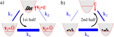
Figure 1: (Color online) Illustration of the model system. Initially, all particles are located on the upper site ($i=0$) which represents the “shuttle”. In the first half of the cycle (a) the on-site potential $v_{0}=\varepsilon$ is raised adiabatically slow from a very negative initial value and the particles are mainly transported via the $k_{1}$ bond to the “canal” which is represented by the strongly coupled canal sites ($i=1,2$). In the second half of the cycle (b) the bias in the coupling is inverted and the particles are mainly transported back from the canal to the shuttle via the $k_{2}$ bond.

II The Bose-Hubbard trimer model

The simplest model that captures the physics of quantum stirring is the three-site Bose-Hubbard Hamiltonian (BHH) BHK07 ; HKG06 ; FP03 (see Fig. 1). This minimal model contains all the generic ingredients of large BHH lattices and therefore often is used as a prototype model in many recent studies HKG06 ; BHK07 ; SAZ07 . A classical analysis of this model has been performed in FP03 ; HKG06 where it was shown that for appropriate system parameters and initial conditions chaotic dynamics would emerge. In this work we consider adiabatic driving of the ground state preparation and therefore chaotic motion is not an issue.

We consider the site index of the quantum trimer taking values $i=0,1,2$. The ${i{=}0}$ site has a potential energy ${v_{0}=\varepsilon}$ and is regarded as a “shuttle”, while the ${i{=}1{,}2}$ sites are regarded as a two level “canal” (with ${v_{1}{=}v_{2}{=}0}$). The corresponding $N$-boson BHH is:

$$\mathcal{H} = \sum_{i=0}^{2}v_{i}{\hat{n}}_{i}+\frac{U}{2}\sum_{i=0}^{2}{\hat{n}}_{i}({\hat{n}}_{i}-1)-k_{c}({b}_{1}^{\dagger}{b}_{2}+{b}_{2}^{\dagger}{b}_{1})$$ (1)

$$-k_{1}({b}_{0}^{\dagger}{b}_{1}+{b}_{1}^{\dagger}{b}_{0})-k_{2}({b}_{0}^{\dagger}{b}_{2}+{b}_{2}^{\dagger}{b}_{0}).$$

Without loss of generality we use mass units such that ${\hbar{=}1}$, and time units such that intra canal hopping amplitude is ${k_{c}{=}1}$. Accordingly the two single particle levels of the canal are $\varepsilon_{\pm}=\pm 1$. The annihilation and creation operators ${b}_{i}$ and ${b}_{i}^{\dagger}$ obey the canonical commutation relations $[{b}_{i},{b}_{j}^{\dagger}]=\delta_{i,j}$ while the operators ${\hat{n}}_{i}={b}_{i}^{\dagger}{b}_{i}$ count the number of bosons at site ${i}$. The interaction strength between two atoms in a single site is given by $U=4\pi\hbar^{2}a_{s}V_{\mbox{\tiny eff}}/\mathsf{m}$ where $V_{\mbox{\tiny eff}}$ is the effective volume, $\mathsf{m}$ is the atomic mass, and $a_{s}$ is the $s$-wave scattering length.

The couplings between the shuttle and the two ends of the canal are $k_{1}$ and $k_{2}$. We assume that both are much smaller than $k_{c}$ Their inverse $1/k_{1}$ and $1/k_{2}$ are like barrier heights, and changing them is like switching valves on and off. It is convenient to define the two control parameters of the pumping as

$$X_{1}=\left(\frac{1}{k_{2}}-\frac{1}{k_{1}}\right),\qquad X_{2}=\varepsilon.$$ (2)

By periodic cycling of the parameters $(X_{1},X_{2})$ we can induce a circulating current in the system. We further discuss this controlled stirring process in the next section.

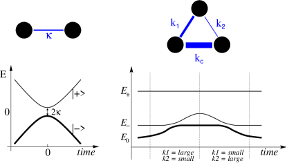
Figure 2: (Color online) Scheme of the avoided crossings for the one particle problem. Left panels: The two-site system (71) is prepared with one particle in the ground state which initially corresponds to having the particle occupying the left site. As the potential $\varepsilon$ is raised the particle encounters an avoided crossing. Due to the slowness of the driving it stays in the ground state which implies an adiabatic passage to the right site. Right panels: The three-site trimer system is prepared with one particle in the ground state which initially corresponds to having the particle occupying the shuttle site. As the potential $\varepsilon$ is varied the particle encounters avoided crossings with the lower canal orbital. A full stirring cycle consists of an adiabatic passage through $k_{1}$ in the first half of the cycle, and another adiabatic passage through $k_{2}$ in the second half of the cycle. See the text for further explanations.

III Stirring

By periodic cycling of the parameters $(X_{1},X_{2})$ we can imitate a classical peristaltic mechanism and obtain a non-zero amount ($Q$) of transported atoms per cycle. During the driving cycle the total number of bosons remains constant. The energy is not a constant of motion, but in the adiabatic limit considered here, the system returns to the same state at the end of each cycle.

The pumping cycle is illustrated in Figs. 1-3. Initially all the particles are located in the shuttle which has a sufficiently negative on-site potential energy ($X_{2}<0$). In the first half of the cycle the coupling is biased in favor of the $k_{1}$ route (${X_{1}>0}$) while $X_{2}$ is raised until (say) the shuttle is empty. In the second half of the cycle the coupling is biased in favor of the $k_{2}$ route (${X_{1}<0}$), while $X_{2}$ is lowered until the shuttle is full. Assuming $U{=}0$, the shuttle is depopulated via the $k_{1}$ route into the lower energy level $\varepsilon_{-}$ during the first half of the cycle, and re-populated via the $k_{2}$ route during the second half of the cycle. Accordingly the net effect is to have a non-zero $Q$.

If we had a single particle in the system, the net effect would be to pump roughly one particle per cycle. If we have $N$ non-interacting particles, the result of the same cycle is to pump roughly $N$ particles per cycle. We would like to know what is the actual result using a proper quantum mechanical calculation, and furthermore we would like to investigate what is the effect of the interatomic interaction $U$ on the result.

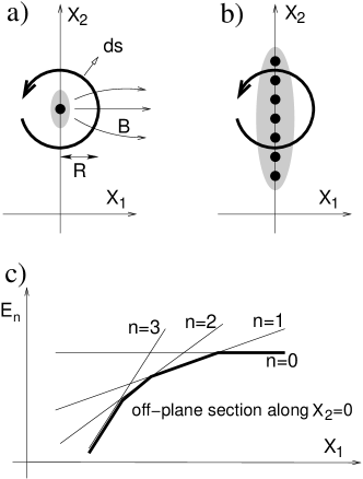
Figure 3: Analysis of the pumping cycle for $N$ particles. See the text for further details. For a large cycle that encircles the whole shaded region we have $Q\approx N$. The position of the “monopoles” is depicted by black dots: (a) no interactions (all monopoles are “piled up” at the same position) (b) with interactions. In panel (c) we schematically plot the energy levels along the $X_{1}=0$ axis for a system corresponding to $N=3$ bosons. Note that energy levels that correspond to non-participating states (those with non-zero occupation of the upper canal orbital) are not plotted.

The above description of the stirring process might look convincing, but in fact it does not hold in the quantum mechanical reality. The quantum stirring process is in general not a peristaltic process but rather a coherent transport effect. This point is best clarified by observing that the simple minded picture above implies that the amount of pumped particles per cycle is at most $N$. This conclusion is wrong. We shall explain in the next section that in principle one can get ${Q\gg N}$ per cycle. The proper way to think about the quantum stirring process is as follows: Changing a control parameter, say $X_{2}$ with some constant rate $\dot{X}_{2}$, induces a circulating current in the system. Each particle can encircle the system more than once during a full cycle. Hence ${Q\gg N}$ is feasible.

IV The adiabatic picture

In analogy with Ohm’s law (where $X$ is the magnetic flux, and $-\dot{X}$ is the electro motive force), the current is ${I=-G_{1}\dot{X}_{1}}$ if we change $X_{1}$ and ${I=-G_{2}\dot{X}_{2}}$ if we change $X_{2}$, where $G_{1}$ and $G_{2}$ are elements of the geometric conductance matrix. Accordingly

$$Q=\oint\limits_{\mbox{\tiny cycle}}Idt=-\oint(G_{1}dX_{1}+G_{2}dX_{2}).$$ (3)

In order to calculate the geometric conductance we use the Kubo formula approach to quantum pumping pmc which is based on the theory of adiabatic processes Berry . It turns out that in the strict adiabatic limit $G$ is related to the vector field $\mathbf{B}$ also known as “two-form” in the theory of Berry phase. Namely, using the notations ${\mathbf{B}_{1}=-G_{2}}$ and ${\mathbf{B}_{2}=G_{1}}$ we can rewrite Eq.(3) as

$$Q=\oint\mathbf{B}\cdot d\vec{s},$$ (4)

where we define the normal vector $d\vec{s}=(dX_{2},-dX_{1})$ as illustrated in Fig. 3. The advantage of this point of view is in the intuition that it gives for the result: $Q$ is related to the flux of a field $\mathbf{B}$ which is created by “magnetic charges” in $X$ space. For $U{=}0$ all the magnetic charge is concentrated in one point. As the interaction $U$ becomes larger the “magnetic charge” disintegrates into $N$ elementary “monopoles” (see Fig. 3). In practice the calculation of $\mathbf{B}$ is done using the following formula:

$$\mathbf{B}_{j}=\sum_{n\neq n_{0}}\frac{2\ {\rm Im}[\mathcal{I}_{n_{0}n}]\ \mathcal{F}^{j}_{nn_{0}}}{(E_{n}-E_{n_{0}})^{2}},$$ (5)

where the current operator is conveniently defined as

$$\mathcal{\mathcal{I}} \equiv \frac{1}{2}(\mathcal{I}_{0\mapsto 1}+\mathcal{I}_{2\mapsto 0})$$ (6)

$$= \frac{i}{2}\left[k_{1}({b}_{0}^{\dagger}{b}_{1}-{b}_{1}^{\dagger}{b}_{0})+k_{2}({b}_{2}^{\dagger}{b}_{0}-{b}_{0}^{\dagger}{b}_{2})\right],$$

while the generalized force operators are defined as

$$\mathcal{F}^{j}\ \ =\ \ -\frac{\partial\mathcal{H}}{\partial X_{j}}$$ (7)

and are associated with the control parameters $X_{j}$. The index $n$ distinguishes the eigenstates of the many-body Hamiltonian. We assume from now on that $n_{0}$ is the BEC ground state.

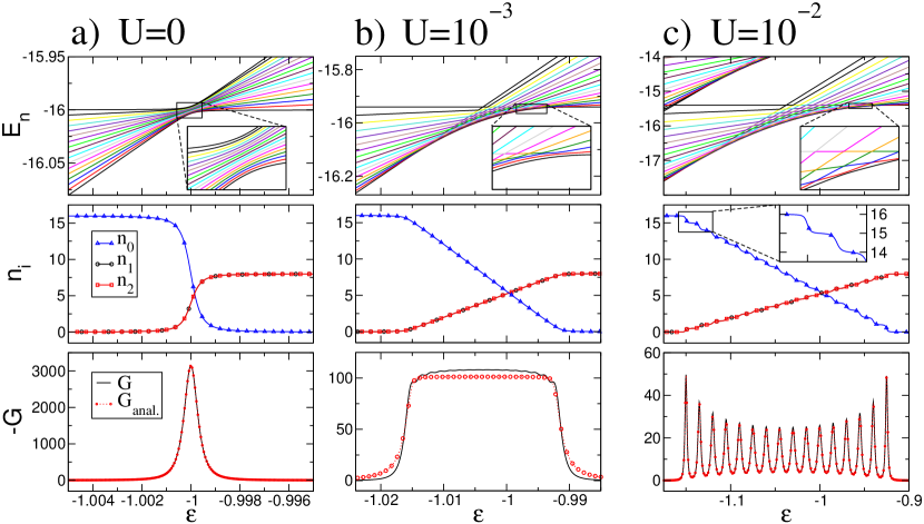
Figure 4: (Color online) Evolution of the energy levels, the site occupation and the conductance for $N=16$ particles and $k_{1}=2\times 10^{-4},\;k_{2}=1\times 10^{-4}$. We refer to three representative values of $U$, which are indicated on top of each set of panels. Upper panels: the lowest $N+1$ energy levels $E_{n}$ which dominate the conductance $G_{2}$ are plotted as a function of $X_{2}=\varepsilon$. The insets represent magnifications of the indicated areas. Middle panels: the site occupations $n_{0}$(blue $\Delta$), $n_{1}$(black $\circ$), $n_{2}$(red $\Box$). Note the steps of size $1$ for the dot-occupation and $1/2$ in the wire-sites occupation in subfigure (c). Lower panels: the corresponding conductance $G_{2}$ as a function of $\varepsilon$. Numerical results are represented by solid black lines while the dotted red line corresponds to the analytical result (95) in (a) and to (103) in (b), (c).

V The two-orbital approximation

We assume an adiabatic process that involves only two orbitals: the shuttle orbital and the orbital of the lower canal level (see right panel of Fig. 2). Accordingly we can simplify the Hamiltonian in a way that illuminates the physics of the quantum stirring process and simplifies the formal treatment. For pedagogical reasons we consider first the single particle ($N{=}1$) case, and extend the calculation to the many-body case in the next section. The model Hamiltonian in the position basis is:

$$\mathcal{H}=\left(\begin{array}[]{ccc}\varepsilon&-k_{1}&-k_{2}\\ -k_{1}&0&-1\\ -k_{2}&-1&0\end{array}\right).$$ (11)

The current can be measured on the $0\mapsto 1$ bond or on the $2\mapsto 0$ bond, accordingly:

$$\mathcal{\mathcal{I}}_{0\mapsto 1} = \left(\begin{array}[]{ccc}0&-ik_{1}&0\\ ik_{1}&0&0\\ 0&0&0\end{array}\right),$$ (15)

$$\mathcal{\mathcal{I}}_{2\mapsto 0} = \left(\begin{array}[]{ccc}0&0&ik_{2}\\ 0&0&0\\ -ik_{2}&0&0\end{array}\right).$$ (19)

For zero couplings (${k_{1}=k_{2}=0}$) the eigenenergies of the orbitals are ${\varepsilon_{\pm}=\pm 1}$ and ${\varepsilon_{0}=\varepsilon}$. The corresponding eigenstates are

$$|\varepsilon_{0}\rangle=\left(\begin{array}[]{c}1\\ 0\\ 0\end{array}\right),\,\,\,\,\,\,|\varepsilon_{-}\rangle=\frac{1}{\sqrt{2}}\left(\begin{array}[]{c}0\\ 1\\ 1\end{array}\right),$$ (26)

$$|\varepsilon_{+}\rangle=\frac{1}{\sqrt{2}}\left(\begin{array}[]{c}0\\ 1\\ -1\end{array}\right).$$ (30)

The Hamiltonian and the current operators in this orbital basis are:

$$\mathcal{H}=\left(\begin{array}[]{ccc}\varepsilon&-\kappa&-\lambda\kappa\\ -\kappa&-1&0\\ -\lambda\kappa&0&1\end{array}\right)$$ (34)

and

$$\mathcal{\mathcal{I}}_{0\mapsto 1}=\frac{k_{1}}{k_{1}+k_{2}}\left(\begin{array}[]{ccc}0&-i\kappa&-i\kappa\\ i\kappa&0&0\\ i\kappa&0&0\end{array}\right),$$ (38)

$$\mathcal{\mathcal{I}}_{2\mapsto 0}=\frac{k_{2}}{k_{1}+k_{2}}\left(\begin{array}[]{ccc}0&i\kappa&-i\kappa\\ -i\kappa&0&0\\ i\kappa&0&0\end{array}\right).$$ (42)

where the effective coupling between the shuttle orbital and the lower canal orbital is

$$\kappa=\frac{k_{1}+k_{2}}{\sqrt{2}}$$ (43)

and the net “splitting ratio” is cnb

$$\lambda=\frac{k_{1}-k_{2}}{k_{1}+k_{2}}.$$ (44)

The stirring cycle starts with all particles localized in the shuttle orbital and the adiabatic particle transport takes place during the avoided crossing of this orbital with the lower canal orbital. Accordingly, we focus on the upper left ($2\times 2$) submatrix:

$$\mathcal{H}=\left(\begin{array}[]{cc}\varepsilon&-\kappa\\ -\kappa&-1\end{array}\right).$$ (47)

In practice it is more convenient to define the averaged current operator ${\mathcal{I}\equiv(\mathcal{I}_{0\mapsto 1}+\mathcal{I}_{2\mapsto 0})/2}$ whose matrix representation is

$$\mathcal{I}=\frac{\lambda}{2}\left(\begin{array}[]{cc}0&-i\kappa\\ i\kappa&0\end{array}\right).$$ (50)

The advantage of this definition is that within the two halves of a symmetric pumping cycle, while $\varepsilon$ is raised or lowered, the same amount of particles is being transported. Thus in order to get $Q$ for a full cycle, we simply double the integrated current over a half cycle, where the variation of the control parameter $\varepsilon$ is monotonic starting from a very negative initial value. For completeness we also write the matrix representation of the generalized force that is conjugate to ${X_{2}=\varepsilon}$

$$\mathcal{F}=\left(\begin{array}[]{cc}1&0\\ 0&0\end{array}\right).$$ (53)

The above expressions for $\mathcal{H}$ and $\mathcal{I}$ and $\mathcal{F}$ completely define the transport problem in the case of one particle. Within the two orbital approximation the calculation of $Q$ therefore reduces to the study of a single LZ crossing, which we discuss in Section VII.

VI The adiabatic variation of the many-body levels

We now turn to the analysis of the many-body problem. The first step is to understand the evolution of the eigenenergies $E_{n}$ as $\varepsilon$ is varied, while the other parameters are kept constant. It is convenient to rewrite the BHH as

$$\mathcal{H} = \mathcal{H}_{\mbox{\tiny shuttle}}(\varepsilon)+\mathcal{H}_{\mbox{\tiny canal}}+\mathcal{H}_{\mbox{\tiny cpl}}$$ (54)

$$\mathcal{H}_{\mbox{\tiny shuttle}} = \frac{U}{2}\hat{n}_{0}(\hat{n_{0}}{-}1)+\varepsilon\hat{n}_{0}$$

$$\mathcal{H}_{\mbox{\tiny canal}} = \frac{U}{2}[\hat{n}_{1}(\hat{n}_{1}{-}1)+\hat{n}_{2}(\hat{n}_{2}{-}1)]-({b}_{2}^{\dagger}{b}_{1}+{b}_{1}^{\dagger}{b}_{2})$$

$$\mathcal{H}_{\mbox{\tiny cpl}} = -k_{1}({b}_{0}^{\dagger}{b}_{1}+{b}_{1}^{\dagger}{b}_{0})-k_{2}({b}_{0}^{\dagger}{b}_{2}+{b}_{2}^{\dagger}{b}_{0}),$$

while the operators for the current and the generalized force are

$$\mathcal{\mathcal{I}}_{0\mapsto 1} = ik_{1}({b}_{1}^{\dagger}{b}_{0}-{b}_{0}^{\dagger}{b}_{1})$$

$$\mathcal{\mathcal{I}}_{2\mapsto 0} = ik_{2}({b}_{0}^{\dagger}{b}_{2}-{b}_{2}^{\dagger}{b}_{0})$$

$$\mathcal{\hat{F}} = -\hat{n}_{0}.$$ (55)

In what follows we assume $0<k_{1},k_{2}\ll k_{c}=1$, and $N|U|\ll k_{c}=1$, and consequently generalize the “two orbital approximation” of the previous section to the case of ${N>1}$ particles.

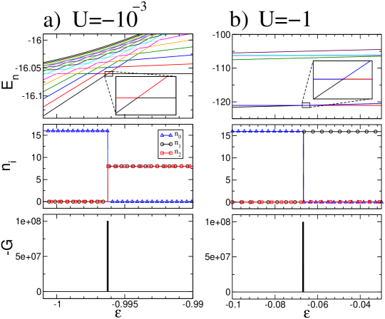
Figure 5: (Color online) Evolution of the energy levels, the site occupation and the conductance for strong attractive interaction $U=-1$ (see Fig. 4 for legend and parameters). The particles are “glued together” and roll like a classical ball from the shuttle to the left wire site as can be seen from the middle panel where the site occupations $n_{0}$(blue $\Delta$), $n_{1}$(black $\circ$), $n_{2}$(red $\Box$) are plotted. The width of the transition is exponentially small in $N$, as explained in the text, and therefore cannot be resolved numerically.

In the zeroth order approximation $k_{1}$ and $k_{2}$ are neglected; later we take them into account as a perturbation. For ${k_{1}=k_{2}=0}$ the number ($n$) of particles in the shuttle becomes a good quantum number. The other ${N{-}n}$ particles occupy the lower orbital ($\varepsilon_{-}$) of the canal because we assume $NU\ll k_{c}$. Hence the many-body energies are

$$E_{n}=E_{\mbox{\tiny shuttle}}(n)+E_{\mbox{\tiny canal}}(N{-}n),$$ (56)

where $n{=}0,1,..,N$, and

$$E_{\mbox{\tiny shuttle}} = \varepsilon n+\frac{1}{2}U(n{-}1)n$$ (57)

$$E_{\mbox{\tiny canal}} = -(N{-}n)+\frac{1}{4}U(N{-}n{-}1)(N{-}n).$$ (58)

From the degeneracy condition ${E_{n}-E_{n{-}1}=0}$ (${n{=}1,2,...N}$ is the number of particles in the shuttle) we determine the location of the ${n\mapsto(n{-}1)}$ crossing to be

$$\varepsilon_{n}=-1+\frac{1}{2}U\times(N{-}3n{+}2).$$ (59)

Accordingly, we conclude that the $N$ crossings are distributed within

$$-1-(N{-}1)U\ \ \leq\ \ \varepsilon\ \ \leq\ \ -1+\frac{1}{2}(N{-}1)U.$$ (60)

One can introduce a rescaled control variable $\hat{\varepsilon}$ which reads

$$\hat{\varepsilon}=\frac{\varepsilon+1}{(N-1)U},$$ (61)

and its support is ${-1<\hat{\varepsilon}<1/2}$. The distance between the crossings, while varying the shuttle potential $\varepsilon$, is $(3/2)U$. Once we take $\kappa$ into account we get avoided crossings, whose width we will estimate in the next paragraph.

Within the framework of the two-orbital approximation, the truncated many-body Hamiltonian matrix takes the form

$$\mathcal{H}_{nm}=E_{n}\delta_{n,m}-\kappa_{n}\delta_{n,n\pm 1},$$ (62)

where $n{=}0,\cdots,N$ and the couplings are defined as ${\kappa_{n}=\langle n{-}1|\mathcal{H}|n\rangle}$. For example, in the ${N{=}3}$ case we have

$$\mathcal{H}=\left(\begin{matrix}E_{0}&-\kappa_{1}&0&0\\ -\kappa_{1}&E_{1}&-\kappa_{2}&0\\ 0&-\kappa_{2}&E_{2}&-\kappa_{3}\\ 0&0&-\kappa_{3}&E_{3}\end{matrix}\right).$$ (63)

The calculation of ${\kappa_{n}}$ involves the matrix elements of $b_{i}^{{\dagger}}b_{0}$, leading to

$$\kappa_{n}=[(N+1-n)n]^{1/2}\,\kappa.$$ (64)

An analogous expression applies to the truncated current operator:

$$\mathcal{I}=\frac{1}{2}\left(\begin{matrix}0&-i\lambda_{1}\kappa_{1}&0&0\\ i\lambda_{1}\kappa_{1}&0&-i\lambda_{2}\kappa_{2}&0\\ 0&i\lambda_{2}\kappa_{2}&0&-i\lambda_{3}\kappa_{3}\\ 0&0&i\lambda_{3}\kappa_{3}&0\end{matrix}\right).$$ (65)

For large $U$, as $\varepsilon$ is varied, we encounter a sequence of distinct LZ transitions:

$$|3\rangle\,\,\,\,\overset{\kappa_{3}}{\longmapsto}\,\,\,\,|2\rangle\,\,\,\,\overset{\kappa_{2}}{\longmapsto}\,\,\,\,|1\rangle\,\,\,\,\overset{\kappa_{1}}{\longmapsto}\,\,\,\,|0\rangle$$ (66)

The distance between avoided crossings is of order $U$ while their width is

$$\delta\varepsilon_{n}=\kappa_{n}.$$ (67)

The widest crossings are at the center with ${\delta\varepsilon_{n}\sim N\kappa}$. This width should be smaller than the spacing $U$ between avoided crossings, else they merge and we no longer have distinct crossings. The other extreme possibility is to regard $U$ as the perturbation rather than $\kappa$. The width of the one-particle crossing is $\kappa$, and it would not be affected by the many-body interaction as long as the span $NU$ is much smaller than that. We therefore deduce that for repulsive interaction there are three distinct regimes:

$$U\ll\kappa/N$$ mega crossing regime

$$\kappa/N<U<N\kappa$$ gradual crossing regime (68)

$$U\gg N\kappa$$ sequential crossing regime

Accordingly, depending on the ratio $U/\kappa$ we expect different results for $G_{2}(X)$. Indeed in a later section this expectation is confirmed both analytically and numerically (Figs. 4-5). In Fig. 6 we report the integrated density of avoided crossings (IDoS) for various values of $U$, $\kappa$, $\lambda$ and number of bosons $N$. We find that all points fall in the predicted range confirming nicely the scaling relation (61). If $U/\kappa$ is small these avoided crossings merge and cannot be resolved. In a later section we discuss the implied scaling relation for the conductance (Fig. 7).

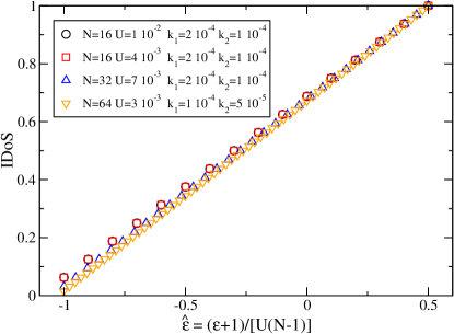
Figure 6: (Color online) Integrated density (IDoS) of avoided crossings (“magnetic monopoles”) for various values of the parameters $U$, $k_{1}$, $k_{2}$ and the boson number $N$ as a function of the rescaled on-site potential $\hat{\varepsilon}$. The support of the IDoS is predicted by Eq. (61) to be $\hat{\varepsilon}=[-1,0.5]$ which is nicely confirmed.

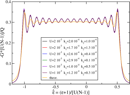
Figure 7: (Color online) Scaling behavior of the conductance $G$ in the gradual crossing regime ($U/\kappa\approx 4.7$). We have $N=16$ particles, and the curves correspond to various values of $\kappa$ and $\lambda$. The $x$-axis is the rescaled control variable $\hat{\varepsilon}$ (61) and the $y$-axis is scaled accordingly to preserve the net charge. Additionally, the ordinate was scaled by the expected charge $Q$ for a half-cycle according to Eq. (96) and indeed the area under the curve is $Q\approx 0.5$. One observes that the curves fall on top of one another which confirms the dependence of $G$ on the ratio $U/\kappa$. Additionally, we overplotted the theoretical expression (solid orange line) for the conductance (103). Although this expression is not expected to be valid in the intermediate regime, the agreement is pretty good. Also the agreement with the estimation from Eq. (104) corresponding to a constant value of $-G\approx 0.315$ is apparent.

VII Transport during a LZ crossing

The prototype example for an adiabatic crossing is the LZ problem. In this section we discuss the analysis of the transport during a LZ crossing, while in the next section we shall use the obtained result as a building block for the analysis of the transport during a stirring process. The following treatment assumes a strict adiabatic process. A more advanced treatment that takes into account non-adiabatic transitions can be found in cnb , where also the resulting fluctuations in $Q$ are calculated.

Consider a single particle in a two-site system (see left panels of Fig. 2). The coupling between the sites is $\kappa$ while the on-site potentials are $v_{i}=\pm\varepsilon/2$, where ${i=1,2}$ labels the sites. The Hamiltonian is

$$\mathcal{H}_{ij}=\left(\begin{array}[]{cc}\varepsilon/2&-\kappa\\ -\kappa&-\varepsilon/2\end{array}\right).$$ (71)

At time $t=-\infty$, the control parameter ${X=\varepsilon}$ is very negative and the particle is on the left site ($i=1$). Then $X$ is increased adiabatically and the levels experience an avoided crossing leading to the adiabatic transfer of the particle to the right site ($i=2$). The current operator and the generalized force operator are represented by the matrices

$$\mathcal{I}_{ij}=\left(\begin{array}[]{cc}0&-i\kappa\\ i\kappa&0\end{array}\right)$$ (74)

and

$$\mathcal{F}_{ij}=\left(\begin{array}[]{cc}1/2&0\\ 0&-1/2\end{array}\right).$$ (77)

The instantaneous eigenenergies of the LZ Hamiltonian are labeled as ${n={-}}$ (lower) and ${n{=}+}$ (upper):

$$E_{n}=\mp\frac{1}{2}\Omega$$ (78)

and the associated eigenstates are

$$|E_{-}\rangle = \left(\begin{array}[]{c}\cos({\theta}/{2})\\ \sin({\theta}/{2})\end{array}\right)$$ (81)

$$|E_{+}\rangle = \left(\begin{array}[]{c}-\sin({\theta}/{2})\\ \cos({\theta}/{2})\end{array}\right),$$ (84)

where

$$\Omega = \sqrt{\varepsilon^{2}+(2\kappa)^{2}}$$ (85)

$$\theta = -\arctan\left({2\kappa}/{\varepsilon}\right).$$ (86)

Note that $\theta{=}0$ at ${t{=}-\infty}$ evolves to $\theta{=}\pi$ at ${t{=}\infty}$. The matrix representation of $\mathcal{I}$ and $\mathcal{F}$ in this basis is

$$\mathcal{I}_{nm}=\left(\begin{array}[]{cc}0&-i\kappa\\ i\kappa&0\end{array}\right),$$ (89)

and

$$\mathcal{F}_{nm}=\frac{1}{2}\left(\begin{array}[]{cc}\cos(\theta)&-\sin(\theta)\\ -\sin(\theta)&-\cos(\theta)\end{array}\right).$$ (92)

Now we can use Eq.(5) to obtain the geometric conductance:

$$G(\varepsilon)=\frac{\kappa\sin(\theta)}{\Omega^{2}}=-\frac{2\kappa^{2}}{[\varepsilon^{2}+(2\kappa)^{2}]^{3/2}}.$$ (93)

Since we assume here a strictly adiabatic process we expect $100\%$ transfer efficiency, and indeed:

$$Q\ = \ \int\langle\mathcal{I}\rangle dt\ =\ -\int Gd\varepsilon$$

$$= \ \left.\frac{\varepsilon}{2\sqrt{\varepsilon^{2}+(2\kappa)^{2}}}\right|_{-\infty}^{\infty}\ =\ 1.$$ (94)

For pedagogical reasons, we rederive the result (93) for the conductance $G(\varepsilon)$ in a straightforward way from the Schrödinger equation in Appendix C. This might add to the understanding of the general discussion of quantum stirring presented in a later section.

VIII Transport during stirring:        the case ${\mathbf{U}=0}$

We have realized that the stirring problem of one particle reduces to the LZ-like crossing problem Eqs.(71,74). Disregarding the different on-site energies, the Hamiltonian is the same as in the LZ-problem Eq.(71). The significant difference is related to the current operator. Its multiplication by the splitting ratio $\lambda$ is the fingerprint of the non-trivial topology. We further discuss the physics behind $\lambda$ at the end of this section. On the technical side, all we have to do is to multiply the result obtained in the previous section by this factor. If we have $N$ non interacting Bosons, the result should be further multiplied by $N$, leading to

$$G(X_{1},X_{2})=-\frac{1}{2}N\lambda\frac{2\kappa^{2}}{[(\varepsilon-\varepsilon_{-})^{2}+(2\kappa)^{2}]^{3/2}}.$$ (95)

In this expression $\varepsilon$ is determined by $X_{2}$ and $\lambda$ is determined by $X_{1}$, while $\kappa$ is conveniently regarded as a fixed parameter. For a full cycle we get

$$Q\ \ =\ \ \oint\langle\mathcal{I}\rangle dt\ \ =\ \ N\lambda.$$ (96)

We note that this result assumes a symmetric stirring cycle such that ${k_{1}=k_{\mbox{\tiny large}}}$ and ${k_{2}=k_{\mbox{\tiny small}}}$ in the first half of the cycle, while ${k_{1}=k_{\mbox{\tiny small}}}$ and ${k_{2}=k_{\mbox{\tiny large}}}$ in the second half of the cycle. Accordingly

$$Q\ \ =\ \ N\frac{k_{\mbox{\tiny large}}-k_{\mbox{\tiny small}}}{k_{\mbox{\tiny large}}+k_{\mbox{\tiny small}}}.$$ (97)

It is more illuminating to denote the $X_{1}$-radius of the pumping cycle by $R$ , as illustrated in Fig. 3 and to re-write the latter expression as follows:

$$Q=N\frac{[1+(\kappa R)^{2}]^{1/2}-1}{\kappa R}.$$ (98)

In particular for small cycles we get a linear dependence on the radius

$$Q\ \ \approx\ \ N\kappa R,$$ (99)

while for large cycles we obtain the limiting value

$$Q\ \ \approx\ \ N.$$ (100)

In a two-site topology the amount of particles that are transported during a strictly adiabatic LZ crossing is exactly $N$. In contrast to that, in the stirring problem that we study, we have non trivial “ring” topology, and therefore $Q$ is multiplied by the splitting ratio $\lambda$. In practice $k_{1}$ and $k_{2}$ are positive and accordingly ${|\lambda|<1}$. But in principle we can have ${|\lambda|>1}$. This would happen if $k_{1}$ and $k_{2}$ were negative. In such case the lower orbital of the “canal” is anti-symmetric rather than symmetric. Going through the derivation one observes that the same results apply with

$$\lambda\ \ \mapsto\ \ 1/\lambda.$$ (101)

For small cycles we find

$$Q\ \ \approx\ \ N\left[\kappa R\right]^{-1},$$ (102)

which means that we can circulate ${Q\gg N}$ particles per cycle. This demonstrates our statement that quantum stirring is not a classical-like peristaltic process, but rather a coherent transport effect.

The results above become more transparent if we notice that they reflect the topology of the $(X_{1},X_{2},X_{3})$ space, where $X_{3}$ is a fictitious Aharonov-Bohm flux to which the operator $\mathcal{I}$ is conjugate [see Appendix A]. In this extended space the field $\mathbf{B}$ that appears in Eq.(4) has zero divergence, with the exception of the “Dirac monopoles” which are located at points where $E_{n_{0}}$ has a degeneracy with a nearby level. If the shuttle orbital and the lower orbital of the “canal” have the opposite parity this degeneracy point is located at ${X=(0,\varepsilon_{-},0)}$ which is in the plane of the pumping cycle. But if the shuttle orbital and the lower orbital of the “canal” have the same parity, then this degeneracy point is displaced off-plane. Accordingly we get the divergent result Eq.(102) or the non-divergent result Eq.(99). It is important to realize that because of the gauge invariance under the transformation $X_{3}\mapsto X_{3}{+}2\pi$ the degeneracy point is duplicated, leading to a “Dirac chain”. In the far field this chain looks like a charged line, and accordingly in the far field we get Eq.(100) which in leading order is not sensitive to the parity of the orbitals.

If we had only one particle, the degeneracy at the center of the pumping cycle would correspond to a single Dirac monopole. If we have $N$ non-interacting particles we have in fact $N$ Dirac monopoles at the same location. As the interaction $U$ is turned on this “pile” disintegrates into $N$ elementary “monopoles” (see Fig. 3). This will be further discussed in the next section.

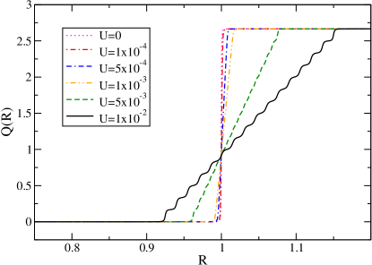
Figure 8: (Color online) Dependence of $Q$ on the $X_{2}$-radius $R$ of the pumping cycle for the system presented in Fig. 4. The curves correspond to different values of the interaction strength $U$ and represent the net amount of particles ($Q$) transported during the first half of a symmetric pumping cycle centered around $X_{2}=\varepsilon=0$. For vanishing interactions $U$ (dotted line) all the particles are transported once the cycle encloses the value $X_{2}=-1$ (mega-crossing). As $U$ is being increased the transport gradually changes leading eventually to a step-like behavior (solid line) for large repulsive interactions (sequential crossing).

IX Transport during stirring:      the case ${\mathbf{U}\neq 0}$

If we have a rectangular pumping cycle in $X$-space, it can be closed at $X_{2}=\pm\infty$, where the influence of the change in $X_{1}$ can be safely neglected since the monopoles are located on the $X_{1}=0$ axis around $\varepsilon\approx-1$. Accordingly, the predominant contribution to $Q$ results from the $dX_{2}$ variation and therefore we refer from now on to ${G(\varepsilon)\equiv G_{2}(X)}$ only. An overview of the numerical results for the conductance is shown in Figs. (4-5), where we plot $G$ as a function of ${X_{2}=\varepsilon}$ for various interaction strengths $U$. Besides $G$ we also plot the $X_{2}$-dependence of the energy levels and of the site population. Five representative values of $U$ are considered including also the case of weak/strong attractive interactions $U<0$. Finally, in Fig. 8 we plot the implied dependence of $Q$ on the radius of the pumping cycle, again for several representative values of $U$.

IX.1 Mega crossing

For small positive values of $U$, the dynamics appears to be the same as in the $U=0$ case. Namely, all the particle cross “together” from the shuttle orbital to the $\varepsilon_{-}$ canal orbital. We call this type of dynamics “mega crossing”. In the language of the adiabatic picture this means that all the Dirac monopoles are piled up in the center of the pumping cycle. Once the interaction $U$ is turned on this “pile” disintegrates into $N$ elementary “monopoles”. Consequently the dependence of $Q$ on the radius of the pumping cycle becomes of importance. Disregarding fluctuations that reflect discreteness of the magnetic charge, the value of $Q$ is determined by the number of monopoles that are encircled by the pumping cycle. Thus, by measuring $Q$ versus $R$ we obtain information on the distribution of the monopoles and hence on the strength of the interatomic interactions.

IX.2 Sequential crossing

In the sequential crossing regime the transport can be regarded as a sequence of LZ crossings. Each LZ crossing is formally the same as the LZ crossing of a single particle in a two-site system, while the topology is reflected by the splitting ratio $\lambda$ and the interaction is reflected in the scaled coupling constants $\kappa_{n}$. Accordingly we get

$$G=-\frac{1}{2}\lambda\sum_{n=1}^{N}\frac{2\kappa_{n}^{2}}{[(\varepsilon-\varepsilon_{n})^{2}+(2\kappa_{n})^{2}]^{3/2}}.$$ (103)

We overplot this formula in the lower panel of Fig. 4c where an excellent agreement is observed.

IX.3 Gradual crossing

For intermediate values of $U$ (weak repulsive interaction), i.e. in the range $\kappa/N\ll U\ll N\kappa$, we find neither the sequential crossing of Eq. (103), nor the mega-crossing of Eq. (95), but rather a gradual crossing. Namely, in this regime, over a range $\Delta X_{2}=(3/2)(N{-}1)U$ we get a constant geometric conductance:

$$G\,\,\,\,\approx\,\,\,\,-\lambda\frac{1}{3U}$$ (104)

which reflects in a simple way the strength of the interaction. This formula has been deduced by extrapolating Eq. (103), and then was validated numerically (see lower panel of Fig. 4b). In this regime it is more illuminating to plot the scaled conductance

$$\hat{G}(\hat{\varepsilon})\ \ \equiv\ \ \left[\frac{Q}{(N{-}1)U}\right]^{-1}\,G(\varepsilon)$$ (105)

which is implied by the scaling (61) of $\varepsilon$. The numerical results are reported in Fig. 7. The shape of the plot depends only on the dimensionless parameters $U/\kappa$ and $N$. The curves corresponding to different $\lambda$ and $U$ values (but with the same constant ratio $U/\kappa$) fall nicely one onto the other with good accuracy, confirming the scaling relation (105).

IX.4 Attractive interaction

So far we have discussed repulsive interactions for which the $N$-fold “degeneracy” of the $U=0$ mega crossing is lifted and we get a sequence of $N$ avoided crossings. Also for $U<0$ this $N$-fold “degeneracy” is lifted, but in a different way: The levels separate in the “vertical” (energy) direction (see upper panels of Fig. 5) rather than “horizontally” (see upper panels of Fig. 4).

In the $U<0$ regime all the particles execute a single two-level transition from the shuttle to the canal (see Fig. 5a). This transition happens directly from the ${n=N}$ state to the ${n=0}$ state. The coupling between these two states is exponentially small in $N$ because it requires a virtual $N$-th order transition in perturbation theory via the intermediate $n$ values.

For sufficiently strong attractive interactions (${|NU|\gg 1}$) all the particles are glued together and behave like a classical ball that rolls from the shuttle to one of the canal sites (see Fig. 5b). When the sign of $X_{1}$ is reversed the ball rolls from one end of the canal to the other end (not shown). This has to be clearly distinguished from the $N$-fold degenerated transition to the lower canal level which is observed in the $U{=}0$ case.

X Conclusions

In this paper we have considered the transport induced in a few site system that contains condensed particles. One new aspect that has emerged throughout the analysis is the existence of four distinct dynamical regimes depending on the strength of the interatomic interactions. This observation also applies to studies of LZ crossings in dimer systems and has further implications regarding the quantum stirring in topologically non-trivial systems. It should be clear that the analysis of our “driven vortex” requires the toolbox of adiabatic processes, and it should be distinguished from the ignited stirring of Refs. RK99 ; MCWD00 .

The actual measurement of induced neutral currents poses a challenge to experimentalists. In fact, there is a variety of techniques that have been proposed for this purpose. For example one can exploit the Doppler effect at the perpendicular direction, which is known as the rotational frequency shift doppler .

The analysis of the prototype trimer system reveals the crucial importance of interactions. The interactions are not merely a perturbation but determine the nature of the transport process. We expect the induced circulating atomic current to be extremely accurate, which would open the way to various applications, either as a new metrological standard, or as a component of a new type of quantum information or processing device.

Appendix A The Berry phase and the $\mathbf{B}$-field

In this Appendix we explain how the field $\mathbf{B}$ emerges in the theory of Berry phase. In the presentation below we follow the notations as in pmc . Given a time dependent Hamiltonian $\mathcal{H}(X(t))$ where ${X=(X_{1},X_{2},X_{3})}$ are control parameters it is convenient to expand the evolving wavefunction in the adiabatic basis

$$\Big{|}\Psi(t)\Big{\rangle}=\sum_{n}a_{n}(t)\Big{|}n(X(t))\Big{\rangle}.$$ (106)

Then the Schrödinger equation $i\partial_{t}\left|\psi\right\rangle=\mathcal{H}(X(t))\left|\psi\right\rangle$ becomes

$$\frac{da_{n}}{dt}=-iE_{n}a_{n}+i\sum_{m}\sum_{j}\dot{X}_{j}A_{nm}^{j}a_{m},$$ (107)

where we defined

$$A_{nm}^{j}=i\Big{\langle}m\Big{|}\frac{\partial}{\partial X_{j}}n\Big{\rangle}.$$ (108)

Differentiation by parts of $\partial_{j}\langle m(X)|n(X)\rangle=0$ implies that $A_{nm}^{j}$ is a Hermitian matrix. We denote its (real) diagonal elements as

$$\mathbf{A}^{j}(X)\ \ \equiv\ \ A_{nn}^{j}.$$ (109)

The line integral over the vector field $\mathbf{A}(X)$ along a closed driving cycle gives the Berry phase

$$\mbox{BerryPhase}=\oint\mathbf{A}\cdot dX.$$ (110)

Using $\partial_{X_{j}}\langle m(X)|\mathcal{H}|n(X)\rangle=0$ we find that the off-diagonal elements of $\mathbf{A}_{nm}^{j}$ can be written as

$$A_{nm}^{j}=\frac{i}{E_{m}{-}E_{n}}\Big{\langle}n\Big{|}\frac{\partial\mathcal{H}}{\partial X_{j}}\Big{|}m\Big{\rangle}=\frac{-i\mathcal{F}_{nm}^{j}}{E_{m}{-}E_{n}}.$$ (111)

The “1-form” $\mathbf{A}^{j}$ is formally like a vector potential, and we can associate with it a gauge invariant “2-form” $B^{kj}$ which is formally like a magnetic field:

$$B^{kj} = \partial_{k}\mathbf{A}^{j}-\partial_{j}\mathbf{A}^{k}$$ (112)

$$= -2\mbox{Im}\langle\partial_{k}n|\partial_{j}n\rangle$$

$$= -2\mbox{Im}\sum_{m}\mathbf{A}_{nm}^{k}\mathbf{A}_{mn}^{j}$$

$$= \sum_{m\neq n}\frac{2\,\textrm{Im}[\mathcal{F}_{nm}^{k}\mathcal{F}_{mn}^{j}]}{(E_{m}{-}E_{n})^{2}}.$$

In order to make the magnetic field analogy more transparent we assume that we have three control parameters $(X_{1},X_{2},X_{3})$. Then it is natural to associate with the antisymmetric matrix $B^{kj}$ a field whose components are $\mathbf{B}_{1}=-B^{32}$ and $\mathbf{B}_{2}=B^{31}$ and $\mathbf{B}_{3}=B^{12}$. This $\mathbf{B}(X)$ field has has zero divergence everywhere with the exception of the Dirac monopoles at points of degeneracy. Dirac monopoles have quantized charge such that their flux is an integer multiple of $2\pi$. The Dirac monopoles must be quantized like that, otherwise Stokes’ theorem would imply that the Berry phase is ill-defined.

Appendix B The Kubo formula and the $\mathbf{B}$-field

The Kubo formula is traditionally used in order to calculate the response of a driven system in the linear response regime. Given a time dependent Hamiltonian $\mathcal{H}(X(t))$ the linear DC-response of the system is expressed as

$$\langle\mathcal{F}^{k}\rangle=-\sum_{j}G^{kj}\dot{X}_{j},$$ (113)

where the generalized conductance matrix $G^{kj}$ can be calculated from the Kubo formula. This matrix can be decomposed in a symmetric and an anti-symmetric part which account for the dissipative and non-dissipative effect of the driving respectively. Here we consider a strictly adiabatic driving: Although the energy is not a constant of motion the system returns to the initial state at the end of each cycle. In this case there is no dissipation and thus we consider only the anti-symmetric (“geometric”) part of $G^{kj}$ which is identified as $B^{kj}$. We further illuminate this identification in the next appendix.

In the stirring problem there are two control parameters which we call $X_{1}$ and $X_{2}$, and the current operator $\mathcal{I}=\mathcal{F}^{3}$ is conveniently regarded as conjugate to a fictitious Aharonov-Bohm flux parameter $X_{3}$. If the particles were charged we could regard $X_{3}$ as an actual control parameter; then $\dot{X}_{3}$ would be the electro-motive-force and $G^{33}$ would be the conventional Ohmic conductance. In Section 4 we use simplified indexing, namely $G_{j}=G^{3j}$. Accordingly Eq.(113) leads to Eq.(3) and in the adiabatic limit we obtain Eq.(4) with Eq.(5) which follows from Eq.(112).

Appendix C Alternative derivation for the geometric conductance

The definition of $\mathbf{B}$ in Appendix A illuminates its geometric interpretation in the context of the the Berry phase formalism, but does not help in understanding why it emerges in the linear response calculation as described in Appendix B. For this reason it might be helpful to derive Eq.(93) directly from the Schrödinger equation. For the LZ crossing problem it becomes

$$\frac{d{a}_{n}}{dt}=-iE_{n}a_{n}+i\dot{\varepsilon}\sum_{m}\mathbf{A}_{nm}a_{m},$$ (114)

where $\dot{\varepsilon}$ is a small parameter. Using the explicit expressions Eq.(81) for the adiabatic eigenstates, the definition Eq.(108), and the identities ${\partial_{x}\arctan(x)=1/(1{+}x^{2})}$ and ${\partial\theta/\partial\varepsilon=2\kappa/\Omega^{2}}$ we find

$$A_{mn}=\frac{\kappa}{\Omega^{2}}\left(\begin{matrix}0&-i\cr i&0\end{matrix}\right)$$ (115)

The zero order adiabatic eigenstates of the Hamiltonian $\tilde{\mathcal{H}}=\mathcal{H}-\dot{\varepsilon}\mathbf{A}$ are $|E_{-}\rangle$ and $|E_{+}\rangle$ of Eq.(81). The first order adiabatic eigenstates are found from perturbation theory. In particular the lower state is

$$|-\rangle = |E_{-}\rangle-i\dot{\varepsilon}\frac{\kappa}{\Omega^{3}}|E_{+}\rangle.$$ (116)

It is important to realize that the expectation value of the current operator vanishes in zeroth order. This is because the the zeroth order Hamiltonian $\tilde{\mathcal{H}}$ is time-reversal symmetric. It is the $\dot{\varepsilon}$ perturbation term that breaks the time-reversal symmetry leading to

$$\langle-\mid\mathcal{I}\mid-\rangle=2\dot{\varepsilon}\frac{\kappa^{2}}{\Omega^{3}}.$$ (117)

Using the notation $\langle I\rangle=-G\dot{\varepsilon}$ we see that this result is in agreement with Eq.(93) as expected.

References

- (1) B.P. Anderson et al. , Science 282, 1686 (1998). D. Jaksch et al., Phys. Rev. Lett. 81, 3108 (1998); C. Orzel et al., Science 291, 2386 (2001); M. Greiner et al., Nature 415, 39 (2002); I. Bloch, Nature Phys. 1, 23-30 (2005); R. Folman et al., Phys. Rev. Lett. 84, 4749 (2000).
- (2) W. Hänsel, et al., Nature 413, 498 (2001); P. Hommelhoff, et al., New J. Phys. 7, 3 (2005).
- (3) A. Micheli, et al., Phys. Rev. Lett. 93, 140408 (2004); B. T. Seaman, et al., (2006) [cond-mat/0606625].
- (4) J. A. Stickney, D. Z. Anderson, A. A. Zozulya, Phys. Rev. A 75, 013608 (2007).
- (5) J. Schmiedmayer, R. Folman, T. Calarco, J. Mod. Opt. 49, 1375 (2002).
- (6) T. Schumm, et al., Nature 1, 57 (2005).; Y-J Wang, et al., Phys. Rev. Lett. 94, 090405 (2005); E. Andersson, et al., Phys. Rev. Lett. 88, 100401 (2002); M. R. Andrews, et al., Science 275, 637 (1997).
- (7) M. O. Mewes, et al., Phys. Rev. Lett. 78, 582 (1997); E. W. Hagley, et al., Science 283, 1706 (1999); Y. Shin, et al., Phys. Rev. Lett. 92, 050405 (2004).
- (8) T. Stoferle, H. Moritz, C. Schori, M. Kohl, T. Esslinger, Phys. Rev. Lett. 92, 130403 (2004); C. Schori, T. Stoferle, H. Moritz, M. Kohl, T. Esslinger, Phys. Rev. Lett. 93, 240402 (2004).
- (9) C. Kollath, A. Iucci, T. Giamarchi, W. Hofstetter, U. Schollwöck, Phys. Rev. Lett. 97, 050402 (2006); A. Iucci, M. Cazalilla, A. Ho, T. Giamarchi, Phys. Rev. A 73, 041608(R) (2006); A.M. Rey, P. B. Blakie, G. Pupillo, C. Williams, C. W. Clark, Phys. Rev. A 72, 023407 (2005); G. G. Batrouni, F. F. Assaad, R. T. Scalettar, P. J. H. Denteneer, Phys. Rev. A 72, 031601(R) (2005); E. Lundh, Phys. Rev. A 70, 061602(R) (2004).
- (10) M. Jääskeläinen, P. Meystre, Phys. Rev A 73, 013602 (2006); D. R. Dounas-Frazer, L. D. Carr, quant-ph/0610166 (2006); K. W. Mahmud, H. Perry, W. P. Reinhardt, J. Phys. B 36, L265 (2003); M. Albiez et al., Phys. Rev. Lett. 95, 010402 (2005).
- (11) B. Wu and J. Liu, Phys. Rev. Lett. 96, 020405 (2006); J. Liu, B. Wu, Q. Niu, Phys. Rev. Lett. 90, 170404 (2003).
- (12) C.-S. Chuu, et. al, Phys. Rev. Lett. 95, 260403 (2005); A. M. Dudarev, M. G. Raizen, and Q. Niu, Phys. Rev. Lett. 98, 063001 (2007).
- (13) L. Amico, A. Osterloh, F. Cataliotti, Phys. Rev. Lett. 95, 063201 (2005).
- (14) D. J. Thouless, Phys. Rev. B 27 6083 (1983). Q. Niu and D. J. Thouless, J. Phys. A 17 2453 (1984). M. Buttiker, H. Thomas and A Pretre, Z. Phys. B-Condens. Mat., 94, 133-137 (1994). P. W. Brouwer, Phys. Rev. B 58, R10135 (1998). B. L. Altshuler, L. I. Glazman, Science 283, 1864 (1999). M. Switkes, et al., Science 283, 1905 (1999).
- (15) G. Rosenberg and D. Cohen, J. Phys. A 39, 2287 (2006), and further references therein.
- (16) M. Hiller, T. Kottos and D. Cohen, Europhys. Lett. 82, 40006 (2008).
- (17) D. Cohen, Phys. Rev. B 68, 155303 (2003).
- (18) M.V. Berry, Proc. R. Soc. Lond. A 392, 45 (1984). J.E. Avron, A. Raveh and B. Zur, Rev. Mod. Phys. 60, 873 (1988). M.V. Berry and J.M. Robbins, Proc. R. Soc. Lond. A 442, 659 (1993).
- (19) M. Hiller, T. Kottos, and T. Geisel, Phys. Rev. A 73, 061604(R) (2006), and further references therein.
- (20) J. D. Bodyfelt, M. Hiller, and T. Kottos, Europhys. Lett. 78, 50003 (2007).
- (21) R. Franzosi, V. Penna, Phys. Rev. E 67, 046227 (2003); K. Nemoto, et al., Phys. Rev. A 63, 013604 (2000).
- (22) M. Chuchem and D. Cohen, J. Phys. A 41, 075302 (2008).
- (23) K. W. Madison, et al., Phys. Rev. Lett. 84, 806 (2000).
- (24) C. Raman et. al., Phys. Rev. Lett. 83, 2502 (1999).
- (25) I. Bialynicki-Birula and Z. Bialynicka-Birula, Phys. Rev. Lett. 78, 2539 (1997).