The “True” Column Density Distribution in Star-Forming Molecular Clouds

Abstract

We use the COMPLETE Survey’s observations of the Perseus star-forming region to assess and intercompare three methods for measuring column density in molecular clouds: near-infrared extinction mapping; thermal emission mapping in the far-IR; and mapping the intensity of CO isotopologues. Overall, the structures shown by all three tracers are morphologically similar, but important differences exist amongst the tracers. We find that the dust-based measures (near-IR extinction and thermal emission) give similar, log-normal, distributions for the full ($\sim 20$ pc-scale) Perseus region, once careful calibration corrections are made. We also compare dust- and gas-based column density distributions for physically-meaningful sub-regions of Perseus, and we find significant variations in the distributions for those (smaller, $\sim$few pc-scale) regions. Even though we have used ¹²CO data to estimate excitation temperatures, and we have corrected for opacity, the ¹³CO maps seem unable to give column distributions that consistently resemble those from dust measures. We have edited out the effects of the shell around the B-star HD 278942 from the column-density distribution comparisons. In that shell’s interior and in the parts where it overlaps the molecular cloud, there appears to be a dearth of ¹³CO, which is likely due either to ¹³CO not yet having had time to form in this young structure, and/or destruction of ¹³CO in the molecular cloud by the HD 278942’s wind and/or radiation. We conclude that the use of either dust or gas measures of column density without extreme attention to calibration (e.g. of thermal emission zero-levels) and artifacts (e.g. the shell) is more perilous than even experts might normally admit. And, the use of ¹³CO data to trace total column density in detail, even after proper calibration, is unavoidably limited in utility due to threshold, depletion, and opacity effects. If one’s main aim is to map column density (rather than temperature or kinematics), then dust extinction seems the best probe, up to a limiting extinction caused by a dearth of sufficient background sources. Linear fits amongst all three tracers’ estimates of column density are given, allowing us to quantify the inherent uncertainties in using one tracer, in comparison with the others.

1. Introduction

In this paper, it is our goal to use data from the COMPLETE Survey of Star-Forming Regions to assess and intercompare three methods for measuring column density in molecular clouds: near-infrared extinction mapping; thermal emission mapping in the far-IR; and mapping the intensity of CO isotopologues. We wish we could offer a snapshot of volume density, as numerical modelers can, but volume density cannot be mapped from our vantage point on Earth without making very model-dependent assumptions. We discuss the position-position-velocity distribution of material in other papers (e.g. Rosolowsky et al., 2008; Goodman et al., 2008): here we focus solely on the column density distribution. Our aim is to offer insight into the biases of particular techniques, and to provide the best estimates to date of “true” column density distributions in molecular clouds suitable for comparison with current and future numerical simulations.

We focus our discussion on the Perseus molecular cloud complex, which covers nearly 10 square degrees on the sky ($\sim 200$ pc² at 250 pc; Enoch et al., 2006; Hirota et al., 2008). A companion paper to this one (Pineda et al., 2008) includes an historical perspective on the use of dust extinction and emission and of CO isotopologue mapping to study column density in molecular clouds, and it offers an in-depth look at abundance variations in the cloud.

2. Data: Three Maps of Perseus

In the past, three principal methods have been used to chart column density in molecular clouds: (1) extinction mapping, using either star counting (e.g. Barnard, 1927; Cernicharo & Bachiller, 1984; Cernicharo et al., 1985) or color-excess measurements (e.g. Lada et al., 1994); (2) dust-emission mapping, at far-IR through mm–wavelengths (e.g. Schlegel et al., 1998); and (3) mapping integrated intensity of molecular-line emission, usually ¹²CO or ¹³CO on large ($>1$ pc) scales (e.g. Padoan et al., 1999). As noted above, there is a long history of the application of these techniques, and we analyze that history in Pineda et al. (2008).

All three of these methods have now been applied, as part of COMPLETE, to the large ($\sim 10$ deg²) swath of sky in Perseus which has also been surveyed by the Spitzer Space Telescope under the “Cores-to-Disks” (c2d; Evans et al., 2003) Legacy Program. The Perseus maps upon which the analysis in this paper rests can be found in Schnee et al. (2005) and Ridge et al. (2006a, b).

2.1. Extinction Mapping

The extinction map used here is presented in Ridge et al. (2006a). To create the map, COMPLETE collaborators João Alves and Marco Lombardi, applied their “NICER” (Near-Infrared Color Excess method Revisited) method to 2MASS near-infrared maps of Perseus.

As described in Lombardi & Alves (2001), the NICER algorithm calculates extinction values based on the difference between the observed average near-IR color of stars within a sampling box to the stars’ intrinsic average color. As the number of stars in a sampling box is reduced, the uncertainty in the extinction calculated by NICER rises. The details of the tradeoffs between high-resolution/high-uncertainty and low-resolution/low-uncertainty mapping with NICER is discussed in detail by Lombardi et al. (2006). The NICER/2MASS map used here is made with 5′ resolution on a 2.5′ grid, a common resolution to which all data presented in this paper have been smoothed. As shown in Figure 1a, we can measure extinctions from $A_{V}=0$ to 10 mag with typical reliability better than 0.25 mag (Figure 1b), but it remains true that the highest uncertainties ($\sim 0.4$ mag) are in the highest extinction regions ($A_{V}\mathbin{\lower 3.0pt\hbox{$\hbox to0.0pt{\raise 6.0pt\hbox{$\char 62\relax$}\hss}\mathchar 29208\relax$}}10$ mag).

Even though 5′ resolution sounds coarse (especially compared with the 46″ intinsic resolution of the COMPLETE spectral-line maps), it is important to appreciate that earlier, optically-based, extinction mapping methods could never come close to this kind of resolution in high column-density regions. In the $V$-band, for example, even modern star-counting techniques typically fail (as zero stars are present in a counting box) at $A_{V}\mathbin{\lower 3.0pt\hbox{$\hbox to0.0pt{\raise 6.0pt\hbox{$\char 62\relax$}\hss}\mathchar 29208\relax$}}6$ mag (e.g. Cambrésy, 1999). The material with $5\mathbin{\lower 3.0pt\hbox{$\hbox to0.0pt{\raise 6.0pt\hbox{$\char 60\relax$}\hss}\mathchar 29208\relax$}}A_{V}\mathbin{\lower 3.0pt\hbox{$\hbox to0.0pt{\raise 6.0pt\hbox{$\char 60\relax$}\hss}\mathchar 29208\relax$}}10$ mag is exactly the material, when observed with the kind of few-tenths-of-a-pc resolution we have here, that appears most actively engaged in forming stars in Perseus (Kirk et al., 2006; Jørgensen et al., 2006), and it is nearly completely opaque in optical wide-field surveys.

We choose, at this point in time, to use the 2MASS data for our extinction maps, rather than the Spitzer IRAC c2d data for two reasons. First, the 2MASS data cover the full region available in COMPLETE’s molecular line maps, while the IRAC data only span “most” of the region. Second, and more importantly, work is still ongoing (Huard, private communication) on the calibration of IRAC-based extinction maps and on the determination an agreed-upon mid-IR extinction law. In the future, the best extinction maps will likely be constructed from photometric observations spanning the NIR and MIR range. Since the absorption by dust becomes progressively less severe at longer wavelengths, the MIR data will be especially useful for mapping out the structure of very high column density gas.

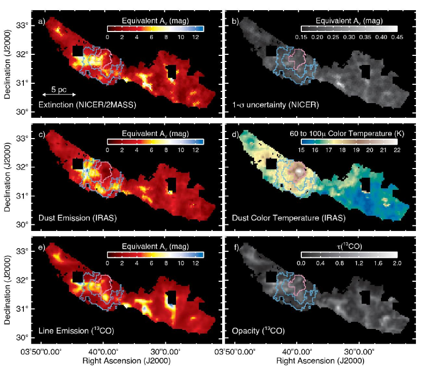
Figure 1.— Maps in the left column show column density as traced by: Extinction (a); Dust Emission (c); and Gas Emission (e). Figure 1b shows the small uncertainties associated with the (NICER) extinction map in Figure 1a. Dust color temperatures based on 60 and 100 µm data are shown in Figure 1d. Note the warm dust associated with the shell around HD278942. The opacity of ¹³CO, which is correlated with column density, is shown in Figure 1f. In all panels, only data points with detections of ¹³CO with S/N$>=5$ are shown, and the resolution is 5′. The IC348 and NGC1333 regions have been excised from the data sets, because all three techniques are biased in cluster regions. The single pink contour surrounds the apparently heated material around HD278942, and the single light blue contour outlined the “overdense” area presumably created by HD278942’s shell, showing the dearth of ¹³CO indicated most clearly in Figure 3. The authors request that this figure be scaled to fill the full width of the page.

2.2. Far-Infrared Emission Mapping

The far infrared data used here are taken from the IRIS (Improved Reprocessing of the IRAS Survey) database (Miville-Deschênes & Lagache, 2005). IRIS represents a substantial improvement over the earlier ISSA release of the IRAS survey, in that it has better zodiacal light subtraction, destriping, calibration and zero level determinations. The importance of finding and using the proper zero level when deriving column density maps where fluxes are not much higher than the noise is explained in Arce & Goodman (2001). For IRAS-based observations of clouds like Perseus, the FIR signal is typically only much greater than the noise above $A_{V}\sim 2$ mag.

Using the IRIS flux maps at 60 and 100 µm, we derive dust temperature and FIR optical depth maps, as explained in Schnee et al. (2005). We use the 2MASS/NICER column density map described in §2.1 to calibrate the conversion between FIR optical depth and NIR extinction. Thus, we fix the overall column density scale with absorption measurements, and then adjust the dust emission properties, given derived color temperatures, to minimize differences beetween absorption and emission probes of dust column. (Note that this procedure assures that the NIR (extinction) vs. FIR (emission) column desnity plots shown in Figure  3 have slope and intercept close to one and zero, respectively.) By comparing Figure 1c, which shows the re-calibrated, IRAS/IRIS-derived “equivalent $A_{V}$” column density map, to the 2MASS/NICER map in Figure 1a, one can see that the point-to-point agreement is good, but far from perfect (see §4). Figure 1d shows the derived color-temperature map (from Schnee et al. 2005) that is used in creating Figure 1c.

Note, as with the choice made for extinction maps, that we have not chosen to use Spitzer maps of thermal emission in the present study. Recently, Schnee et al. (2008) have presented a full analysis of the long wavelength Spitzer MIPS maps of Perseus, in concert with the IRAS-based data used here. The Spitzer map coverage is smaller than the IRAS (all-sky) coverage, and at the resolution of the present study, the results of Schnee et al. (2008) show that the subtle differences between extinctions determined using 60 and 100 microns, and combinations at longer wavelengths are not critical to our analysis here (see histograms in Figure 9 of Schnee et al. 2008).

2.3. Molecular-Line Mapping

The implicit assumption behind mapping column density using molecular line emission is that by integrating emission over all velocities, one can trace out all of the molecular gas along any particular line of sight. This assumption fails when either: 1) a molecular line is only excited under special physical conditions; 2) emission from a particular line becomes optically thick; and/or 3) the species used in an investigation does not have a constant abundance relative to molecular hydrogen. In reality, any one and often all three of these are true (see Pineda et al., 2008). But still, by making a prudent choice of molecular tracer, one can minimize these complicating conditions and use line maps to trace column density.

In the past, researchers (Bachiller & Cernicharo, 1986; Langer et al., 1989) have argued that ¹³CO, which is excited above volume densities $\sim 1000$ cm^-3 (column densities $A_{V}\sim 1$ mag in nearby molecular clouds) remains optically thin throughout “most” of a molecular cloud’s volume, and also remains of relatively constant abundance, except in very cold ($T<15~{}\rm{K}$) dense ($n({\rm H_{2}})>5000$ cm^-3) regions where carbon-bearing species are heavily depleted (Caselli et al., 1999). Therefore, ¹³CO maps are used here as the most relevant molecular line tracer to compare with extinction maps and IRIS-based dust emission maps, which are also sensitive to material at or above about 1 mag.

The full ¹³CO map presented here was made for the COMPLETE Survey at the Five College Radio Astronomy Observatory, and it is described in detail in Ridge et al. (2006a). The full-resolution map was made in on-the-fly (OTF) mode with the 32-element SEQUOIA array, and contains nearly 200,000 independent 46″ pixels. As noted above, we have smoothed the map to 5′ resolution in order to match the column density maps described in §2.1 and §2.2 above. After this smoothing, the average baseline rms in each of the resulting pixels is 0.027 K, and there are just over 3000 pixels (in all the maps in Figure 1). All points with signal-to-noise ratios (based on peak/rms temperature) below 5 in the smoothed map have been excised as less-than-reliable ¹³CO detections.

One of the most common, but not necessarily most accurate, ways to estimate molecular gas column density, $N({\rm H_{2}})$, from ¹³CO emission comes from: adjusting the velocity-integrated intensity of ¹³CO, $W({\rm{}^{13}CO})$ $=\int{T_{A}({\rm{}^{13}CO})dv}$, for telescope efficiency; assuming a uniform excitation temperature; and multiplying by a conversion factor that accounts for the ratio of ${\rm H_{2}}$ to ¹³CO (e.g. Bachiller & Cernicharo, 1986, and references therein).

To make a more accurate calculation of $N({\rm{}^{13}CO})$ one can employ measured kinetic temperatures and optical depths from ¹²CO observations (see Langer et al., 1989). Because COMPLETE includes ¹²CO as well as ¹³CO maps, we can use the observed brightness temperature of ¹²CO to estimate the excitation temperature (assuming that ¹²CO is optically thick), and then calculate a column density map assuming that the levels are populated following a Boltzmann distribution. All maps and graphs relating to ¹³CO column density distributions in this paper, unless explicitly labeled as “W(¹³CO)”, are made in this way (see Ridge et al., 2006a). We also assume a constant abundance, of $3.98\times 10^{5}$, for ${\rm H_{2}}$ relative to ¹³CO, even though some important variations in that ratio do exist, and are studied in detail in Pineda et al. (2008).

Figure 1f shows the opacities derived from the same set of calculations that yields Figure 1e (the column density map). The opacities, many of which significantly exceed unity, are well-correlated with the column density. Once $\tau\gg 1$, any spectral line is no longer a very faithful column density tracer, even when we work arduously to correct for opacity.

In order to convert molecular column density, $N$, to the “equivalent $A_{V}$” units used in this paper, we use the procedure outlined in Pineda et al. (2008), which gives:

$$A_{V}({\rm{}^{13}CO})=4.24\times 10^{-16}N({\rm{}^{13}CO})+1.67~{}.$$ (1)

To facilitate comparison of the present analysis with previous work, Pineda et al. (2008) assume a constant ratio of reddening to extinction, $R_{V}=A_{V}/E(B-V)=3.1$, equal to the measured average value measured for the Galaxy (Bohlin et al., 1978). We note, though, that $R_{V}$ can have values up to $\sim 6$ (Draine, 2003; Goodman et al., 1995), especially in high-density regions. Lastly, we point out that the coefficients in eq. (1) apply to Perseus as a whole, even though we measure them to vary by as much as $\pm 30\%$ from region to region within Perseus (Pineda et al., 2008). We discuss the significance of these regional variations in §4.3 below.

In the bottom panel of Figure 2, we show both the $W({\rm{}^{13}CO})$-based and the $N({\rm{}^{13}CO})$-based histograms of column density. Notice that the $W({\rm{}^{13}CO})$ distribution appears to underestimate the amount of material at low column density (where temperature is typically higher) and at very high column density (where $\tau$ is high). Even after accounting for temperature and opacity variations though, the $N({\rm{}^{13}CO})$ distribution is still dangerous to interpret too literally, because at low $A_{V}$ ($<$3 mag) the gas is sub-thermally excited, and at high extinction the optical depth is significantly larger than $1$ (Pineda et al., 2008). We quantify and discuss the uncertainties in molecular column density as compared with dust measurements below in §4.1.

3. Data Editing

In order to restrict the comparison in this paper to reliable measurements of column density in the portions of molecular clouds not dominated by the localized heating and stirring caused by embedded massive stars we have excluded certain positions from all three data sets compared here. The “exclusion criteria” are as follows.

Points not having reliable measurements in all three tracers are omitted. For ¹²CO and ¹³CO data, we use only positions with signal-to-noise (peak-to-rms) ratios greater than 15 and 5, respectively. Note, though, that even with infinite sensitivity there would still be a minimum detectable column density for the line measurements, due to the fact that a critical density of matter is needed to excite CO or ¹³CO collisionally. (This “minimum” density for excitation is what leads to the additive constant in the relationship between $A_{V}$ and $N({\rm{}^{13}CO})$ shown in eq.. (1). We also exclude any points where the fitted ¹²CO line-width is smaller than 80% of the ¹³CO line-width, because this is indicative of either: 1) multiple velocity components along the line of sight captured by one tracer but not the other; or 2) of an unphysical result caused by marginal data quality.

The IC348 and NGC1333 cluster regions are eliminated, using purely spatial cuts (see black “holes” in Figure 1), from our analysis, because when material is heated non-uniformly from within, it is difficult to derive accurate column densities from either dust or gas emission (see Schnee et al., 2006). We also remove a small number of other pixels with stellar densities high enough (in this case, $>10$ stars/pixel) to imply a significant contribution from stars embedded in Perseus. This is necessary because NICER relies on “background” stars for extinction mapping, and will underestimate extinction if embedded stars are included by accident.

As indicated on the dust temperature map in Figure 1d, a heated shell surrounds the B-star HD 278942, and portions of it overlap with our study region, in projection. The shell is actually located just behind the molecular clouds, and it apparently touches the clouds at a few localized points of contact (see Ridge et al., 2006b). In Figures 1 and 3, we have marked the effects of the shell’s low-density hot interior (in pink), as well as of its over-dense heated rim (in blue). In the histograms of Figure 2 and for the corresponding fits shown in Table 1, the points effected by the shell’s interior and exterior have been excluded. In Figure 3, we show, for illustrative purposes only, the shell interior/exterior points in pink/blue, but we calculate the scatter amongst the different tracers excluding the shell points.

Lastly, positions close to the border of the map are removed when they would be effected by inaccurate convolution.

In summary, all of the positions shown with non-null values in Figure 1 are shown in Figure 3, but the points within the “shell” regions are excluded from the histograms and fits in Figure 2.

4. Results: The Distribution of Column Density in Perseus

Figure 2 compares, as histograms, the distributions of column density implied by the three different techniques (extinction, thermal emission, and molecular lines) under study here. To facilitate comparison with theories that predict a log-normal density distribution (see §5.1), the histograms are shown in linear-log space, where a log-normal appears as a Gaussian. The log-normal least-squares fit to the 2MASS/NICER-based extinction distribution is repeated (in blue) as a fiducial in all plots. Table 1 shows the fit parameters for each column density distribution based on the functional form:

$${\rm Number\ of\ pixels}={\rm Scaling}*\,e^{-(\log A_{V}-\log{A_{V,0}})^{2}/2\sigma^{2}}$$ (2)

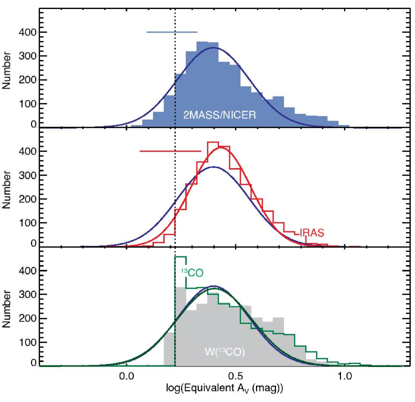
Figure 2.— Pixel-by-pixel column density histograms for the full Perseus COMPLETE data set shown in Figure 1. Note that all tracers are smoothed to a common $5^{\prime}$ resolution, and only points where ¹³CO is reliably detected are included (see text). Each distribution shows the column density as labeled on the plot, converted to units of $A_{V}$, as explained in the text. In every panel, the solid smooth blue curve shows the Gaussian fit to the 2MASS/NICER-based distribution, for reference. The red smooth curve in the middle panel, and the green smooth curve in the lower panel, show Gaussian fits to the IRAS- and ¹³CO-implied distributions, respectively. The grey shaded histogram in the bottom panel shows $W$(¹³CO) converted to units of $A_{V}$, but the fit shown is only for the curve just labeled “¹³CO,” which gives total column density calculated using eq. (1). Fit parameters for all four column density distributions shown in this Figure are given in Table 1. The dashed vertical line extending through all three panels shows the cutoff (lowest) value of column density measurable with ¹³CO, according to eq. (1). The short horizontal bar centered on the dashed line in the top pane shows the $1\sigma$ spread in distribution of $|A_{V}(2MASS)-A_{V}({\rm{}^{13}CO})|/A_{V}({\rm{}^{13}CO})$ and for the middle pane the same dispersion but for $|A_{V}(IRAS)-A_{V}({\rm{}^{13}CO})]/A_{V}({\rm{}^{13}CO})|$. Figure 5 shows the regional breakdown of these same histograms.

Table 1Fit Parameters

Tracer	Scaling	$\log A_{V,0}$	$A_{V,0}$	$\sigma$
$A_{V}$	336$\pm$14	0.397$\pm$0.008	1.18$\pm$0.01	0.163$\pm$0.008
$N_{dust}$	416$\pm$12	0.433$\pm$0.005	1.145$\pm$0.005	0.136$\pm$0.005
$N({\rm{}^{13}CO})$	324$\pm$27	0.40$\pm$0.02	1.19$\pm$0.02	0.17$\pm$0.02
$W({\rm{}^{13}CO})$	298$\pm$18	0.45$\pm$0.01	1.22$\pm$0.02	0.20$\pm$0.01

It might seem surprising, especially given the non-gaussian shape of the ¹³CO histogram, that the $A_{V,0}$ parameter for all the column density tracers are so similar, however, keep in mind that this is to be expected because thermal emission and molecular line data have been calibrated with the 2MASS/NICER-based extinction map.

4.1. Uncertainty Based on Tracer Inter-Comparison

Figure 3 shows direct inter-comparisons of the all three column density measures: extinction, thermal dust emission, and gas emission. The overall scatter around the 1:1 lines can likely be attributed, in large part, to variations along the line of sight of: dust properties; dust temperature; and gas volume density (which effects line emission). We explain below that the principal source of variation between the two dust tracers is variation in temperature along the line of sight; while for comparisons between ¹³CO and dust tracers, variations are caused by changes in the ratio of gas to dust along the line of sight.

Dust emission is dependent on temperature, but extinction is not. By applying radiative transfer calculations to numerical models of molecular clouds, Schnee et al. (2006) showed that most of the scatter in comparing extinction and emission based column density measures is likely caused by line-of-sight variations in dust temperature. Specifically, the scatter in the middle panel of Figure 3 is directly modeled, and explained, by this effect in Schnee et al. (2006), so we will not discuss it further here.

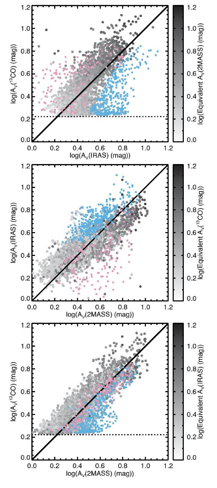
Figure 3.— Inter-comparison of measured column density distributions, all shown in units of $A_{V}$ (see text). The horizontal dotted lines in the top and bottom panels show the minimum column density measurable with ¹³CO corresponding to the additive constant in eq. (1). Note that the grey scale color of the data points shows the “third” measure of column density not plotted on the $x$ or $y$ axis for each plot, so that any points that do not look to be part of a smooth grey gradient are “outliers” in that third measure. Points colored blue and pink correspond to the blue-outlined shell exterior and the pink-outlined shell interior in Figure 1. The pink and blue point are shown here for illustrative value, but they are not included in the histograms in Figures 1 and 5, or in any fits to column density distributions, as explained in the text. The 45-degree lines are not fits: they simply show a 1:1 relationship that might reasonably be expected given that the IRAS-based and ¹³CO-based measures have been calibrated to best match the 2MASS-based $A_{V}$ distribution overall (see text).

To discuss the variations between dust- and gas-based measures of column density, we use Figure 4, which shows a schematic diagram of gas and/or dust structures viewed from various vantage points. The general idea of a “dust-to-gas” ratio is fine as long as one takes care to specify the volume over which that ratio is intended to apply. In other words, if clouds like those shown in the Figure 4 made up a whole galaxy, then summing all the dust and all the gas mass and dividing would be a fine and accurate expression of a volume-averaged dust-to-gas ratio. In our case, however, where we are interested in detailed pixel-by-pixel comparisons of column density measured with either dust or gas, plane-of-the-sky variations in the dust-to-gas ratio matter greatly, but are difficult to treat.

The full “dust-to-gas” ratio derivable from measurements of CO isotopes and extinction relies on the wavelength dependence of extinction and on the abundance of CO isotopes in the gas. As explained in §2.3 and in Pineda et al. (2008), we assume in this paper that the wavelength dependence of extinction is constant (as $R_{V}=A_{V}/E(B-V)=3.1$), and that the abundance of ¹³CO is fixed for all of Perseus, at the value corresponding to the coefficients in eq. (1). We make these assumptions in order to show how gas and dust maps would typically compare, as this approach, or an even less customized one, where dust-to-gas ratios and abundances from the literature are used without testing, is most common. In Pineda et al. (2008) we give a detailed analysis of how much the calibration of dust-to-gas relationships (¹³CO abundance) varies amongst the sub-regions of Perseus under both the linear approximation (eq. (1)) and also with a curve-of-growth approach.

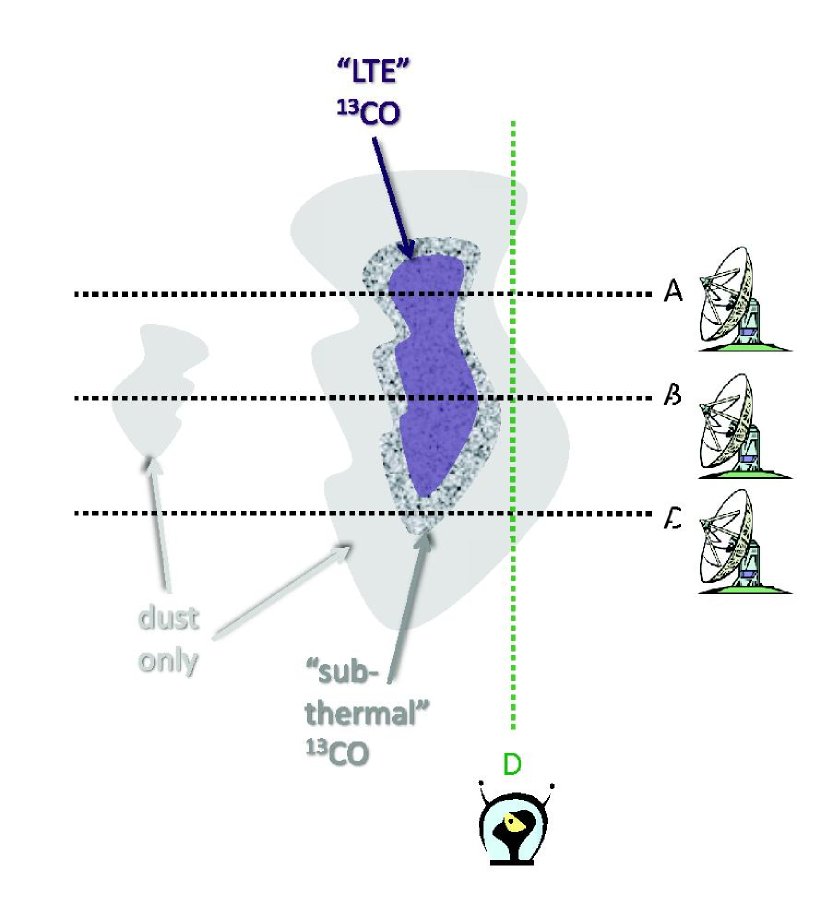
Figure 4.— Schematic diagram showing various lines of sight through various conditions. A, B, and C, are views as seen from our vantage point on Earth. In A, we have the favorable situation where ¹³CO is in near-LTE (shaded purple), and all of the low-density material around it, some of which does not emit in ¹³CO at all (shaded grey), but still shows up in dust measures, is associated with the cloud of interest. In B, the situation is as in A, but an additional region which emits in dust but not in ¹³CO (either due to low density or due to a dearth of ¹³CO) is included. In C, the densest gas the line of sight passes through (shown as marbled grey) is dense enough to excite some ¹³CO, but not at a level truly indicative of the full column density present, because the collisions at this “sub-critical” density are too infrequent. In D, we see an “alien’s view” of the same cloud, which passes through the “dust-only” zones but no ¹³CO emitting regions, even though it crosses A, B, and C.

The ¹³CO(1-0) transition is only excited above a certain critical density, and the transition to “LTE” levels of excitation is actually a gradual one. So, in Figure 4, we show some low-density dusty regions where ¹³CO is not excited at all, some slightly-higher-density regions where it is sub-thermally excited, and some where the density is high enough for near-LTE conditions. Figure 4 clearly shows that while we can excise points with no ¹³CO emission on the plane of the sky, we cannot excise dust along the line of sight that would produce no ¹³CO emission if viewed “from the side” (e.g. by the alien in the Figure).

If all lines of sight in a region were exactly the same as line-of-sight “A” in Figure 4, then: 1) an equation for converting gas to dust column density like eq. (1) could be valid; and 2) there would be no scatter in comparing dust and gas measures of column density. However, in a real cloud like Perseus, some lines of sight pass through additional material that contains dust but does not emit in ¹³CO, as shown for line of sight “B” in Figure 4. That additional material can be background or foreground to the cloud. Or, it can be material within the cloud that is depleted or deficient in ¹³CO, for a variety of reasons.

The ¹³CO column densities given in this paper are calibrated using a single “typical” conversion factor in eq. (1), for all of Perseus. This calibration makes the implicit assumption that the mixture of foreground/background/depleted/deficient material along lines of sight within Perseus does not vary too much, which is not strictly true–and the scatter seen in Figures 2 and 5 is caused primarily by this assumption. Note that since we know that the shell region (highlighted using blue and pink in Figures 1 and 3) is unusual in both its temperature and for its apparent ¹³CO deficiency (see §4.2, below), it has been excised from all fits (including the overall calibration) and histograms (Figures 1 and 5) in this paper.

Equation (1) has an additive factor corresponding to the typical minimum column density at which ¹³CO is detected. This minimum is shown with dotted lines in Figures 2 and 5 at $\log A_{V}=\log 1.67=0.22$. Just as the slope of the gas-to-dust calibration does not universally apply to all lines of sight, neither will this minimum. As explained above, we have excised all positions with ¹³CO levels below the minimum set by eq. (1), but the remaining positions will sometimes give dust-derived extinctions below the gas-derived minimum. The biggest effect causing “leakage,” beyond the low-density cutoff, which is partially responsible for the low-density tails seen in Figures 2 and 5, is simply the scatter about the 1:1 relationships shown in Figure 3. This scatter is characterized by horizontal error bars in Figures 2 and 5, the calculation of which is explained below.

A more subtle effect causing “leakage” below the ¹³CO low column cutoff is also present, and it is illustrated in line of sight “C” in Figure 4, which shows a line of sight that passes through a “sub-thermally excited” region. In cases like “C,” ¹³CO will be detectable, but the density in the region producing the emission is below or barely at the critical density, such that one cannot reliably convert ¹³CO line intensity to a column density using eq. (1). As shown in Pineda et al. (2008), when one uses a more appropriate curve-of-growth fit, rather than a linear approximation, ¹³CO integrated intensity typically rises more steeply than a linear fit to the same data would imply. As a result, a linear conversion (eq. (1)) applied to the observed ¹³CO intensity in low-density (sub-thermally-excited) regions will often overestimate the column density. Thus, some of the positions creating the “low column” tails shown in Figures 2 and 5 are likely to actually be at the low column densities that dust measures: their column density is just overestimated by (sub-thermally-excited) ¹³CO. Note, further, that the seemingly odd pile-up of ¹³CO at densities just above the cutoff in Figure 2 is similarly caused by the linear approximation’s inability to properly treat sub-thermally-excited (relatively low density) gas.

To empirically estimate the scatter associated with all manner of variations in dust and gas properties, we calculate the standard deviation of the distributions of the normalized differences between one column density measure and another at each point in the maps. We find, for the full Perseus map, that that $|A_{V}$(IRAS)-$A_{V}$(2MASS)$|/A_{V}$(2MASS) has 1-sigma width (standard deviation) of 26% and $|A_{V}$(¹³CO)-$A_{V}$(2MASS$)|/A_{V}$(2MASS) has $1\sigma$ width 24%. It is clear from Figure 3 that these standard deviations will be larger than the $1\sigma$ uncertainty in a linear fit, because the 1:1 line (implicitly assumed in the standard deviation calculation) is not a perfect representation of the real relationships between all the extinction measures.

In Figures 2 and 5, we show horizontal bars of varying lengths centered at the threshold value of $\log A_{V}=0.22$ in order to demonstrate that the fluctuations one sees about the 1:1 lines in Figure 3 are large enough to cause the low-column-density tails seen in Figures 2 and 5. The specific length for each horizontal bar shown is the standard deviation of $|A_{V}$(IRAS)-$A_{V}$(¹³CO)$|/A_{V}$(¹³CO) for IRAS-based panels of Figures 2 and 5, and $|A_{V}$(2MASS)-$A_{V}$(¹³CO)$|/A_{V}$(¹³CO) for the 2MASS/NICER-based panels. We discuss the implications of dust and gas probing slightly different regions along the line of sight further in §5.3, below.

4.2. Paucity of ${\rm{}^{13}CO}$ in the Shell Around HD 278942

The overabundance of blue points in the lower-right portion of the two parts of Figure 3 that involve ¹³CO data is likely due to a dearth of ¹³CO in the shell around HD 278942. On the plane of the sky, nearly all of the points that lie below the overall 1:1 trend are associated with the shell (see blue contour in Figure 1). The effect appears most strongly when comparing ¹³CO to dust emission (Fig. 3, top), but we base our statements here on the comparison of ¹³CO and extinction (Fig. 3, bottom), because the shell’s effects also biases the dust emission column density measurements in that region (as shown in the middle panel of Figure 3). We suspect that either the shell structure is young, and molecules, such as ¹³CO, have not had time to form, or that the energetic radiation associated with the shell (see Ridge et al., 2006b) has destroyed pre-existing ¹³CO. In other words, the column density along lines of sight through the shell (outlined in blue in Figure 1) has a molecular component, associated with the (rest of the) Perseus star-forming region, plus a component associated with the shell which contains a lower fraction of molecular gas.

4.3. Regional Variations

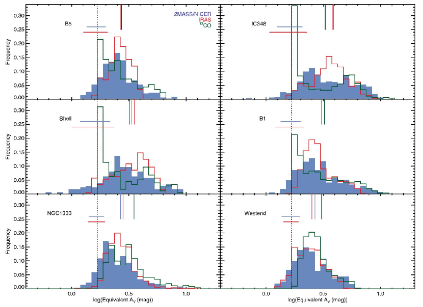
Figure 5.— Regional variations in column density distributions. Each panel shows the same assortment of measured distributions as in Figure 2 only without W(¹³CO). As explained in more detail in Figure 2’s caption and in the text, the vertical dotted line shows the minimum $A_{V}$ measurable with ¹³CO and the short horizontal bars show indicate the characteristic scatter about the relationship between each dust tracer and ¹³CO. Parameters for Gaussian fits to normalized versions of these distributions are given in Table 2. The short vertical lines hanging from the top axis indicate the mean value of extinction for each distribution (by color), and the means of the normalized extinction are given in Table 2. Note that we use “frequency” on the y-axis in these plots, rather than “number” as in Figure 2, to facilitate inter-comparison of the various regions, not all of which include the same total number of positions (see Table 2).

Perseus itself is a large complex of molecular clouds. A division of it into a set of morphologically-distinct sub-regions can be guided by a plot of dust temperature versus gas velocity, as explained in Pineda et al. (2008). Histograms of column density analogous to those shown in Figure 2 are shown in Figure 5 for the same sub-regions (B5, IC348, Shell, B1, NGC1333, and Westend) discussed in Pineda et al. (2008). Significant variation from region to region is clearly present. Typically, each sub-region has of order 500 points (out of $\sim 3500$ for all of Perseus, see Table 2) and has a maximum linear extent of $\sim 5$ pc rather than the $\sim 25$ pc full length of Perseus, making each sub-region a significantly smaller statistical and physical sample than is all of Perseus.

Table 2Regional Variations

Name	Mean $A_{V}$	Mean $\ln{A_{V}}$	Mean $\ln{x}$	Sigma $\ln{x}$
All, Number of Points= 2892
NICER	3.080	1.024	-0.101	0.433
IRAS	3.032	1.052	-0.057	0.329
N(13CO)	3.243	1.076	-0.101	0.427
W(13CO)	3.215	1.083	-0.084	0.404
B5, Number of Points= 344
NICER	2.734	0.940	-0.065	0.349
IRAS	2.692	0.968	-0.022	0.213
N(13CO)	2.850	0.975	-0.073	0.368
W(13CO)	2.733	0.941	-0.065	0.353
IC348, Number of Points= 552
NICER	3.872	1.230	-0.124	0.500
IRAS	3.826	1.279	-0.063	0.359
N(13CO)	3.487	1.105	-0.144	0.525
W(13CO)	3.293	1.068	-0.123	0.496
Shell, Number of Points= 176
NICER	3.318	1.076	-0.123	0.503
IRAS	3.523	1.194	-0.065	0.373
N(13CO)	3.250	1.053	-0.125	0.484
W(13CO)	3.193	1.053	-0.108	0.458
B1, Number of Points= 631
NICER	3.268	1.075	-0.109	0.448
IRAS	3.057	1.068	-0.050	0.304
N(13CO)	3.351	1.086	-0.123	0.477
W(13CO)	3.233	1.069	-0.104	0.450
NGC1333, Number of Points= 642
NICER	2.681	0.915	-0.071	0.358
IRAS	2.813	0.994	-0.041	0.271
N(13CO)	3.445	1.147	-0.090	0.396
W(13CO)	3.518	1.190	-0.068	0.356
Westend, Number of Points= 547
NICER	2.674	0.919	-0.065	0.353
IRAS	2.511	0.879	-0.041	0.285
N(13CO)	2.879	1.021	-0.036	0.259
W(13CO)	3.071	1.089	-0.032	0.250

The shapes of the distributions vary significantly from sub-region to sub-region, and most also show significant disagreement amongst the three column density tracers used here. One key point is that some of the tracer-to-tracer disagreement is caused by (purposely) using only a single CO abundance, and a single form of eq. (1) in creating Figure 5. Had we customized the calibration region-by-region, as is done in Pineda et al. (2008), we could improve the tracer-to-tracer agreement some, but then we would not be representing legitimate sub-sets of the same data shown in Figure 1 through 3. Overall, ¹³CO as a tracer seems most capricious, and we suspect that this is due to significant variations in physical conditions (e.g. temperature, radiation field, region age) other than (column) density that effect its abundance and excitation.

A subtler point concerning variations in distribution shape, both regionally, and tracer-to-tracer, concerns real variations in dust-to-gas ratio, in gas properties (e.g. ¹³CO abundance), and/or in dust properties (e.g. $R_{V}$). We know that these properties vary (cf. §2.3 and Pineda et al., 2008) even on the many-pc scales characteristic of the “regions” we discuss here. So, they likely also vary on smaller scales, meaning that subtle changes in the shape of the distributions seen in Figure 2 and 5 would be apparent if we could account for these variations. In their paper on “Can We Trust the Dust?,” Padoan et al. (2006, see also §5.3, below) suggest that very small-scale variations ($<0.1$ pc) variations in the dust-to-gas ratio may in fact exist. So, in the future, when we can carry out inter-comparisons of column density tracers on even smaller scales than those we consider in this paper, it will be interesting–and potentially important–to quantify how much the dust-to-gas ratio, as well as intrinsic gas and dust properties, change at various scales, and under various conditions.

If we study only the NICER-based histograms in Figure 5, which are not effected by calibration choices here, there are still very significant variations from region to region, and one is left wondering how sample (region) size effects the shape of one of these histograms. We consider this question, and others, in the context of numerical simulations, below.

5. Implications

5.1. Comparisons with Numerical Simulations

In this section, we consider how numerical simulations offer insight into the shape of column density distributions.

Vázquez-Semadeni (1994) shows that for highly supersonic flows where gravitational and magnetic forces become negligible, the gas has a pressureless behavior. Under these conditions, the hydrodynamic equations become scale invariant, i.e., motions at all length and density scales obey the same equations. As a result, the probability density function of the volume density, $n$, is expected to be log-normal. Ostriker et al. (2001) demonstrate that for essentially isotropic flows, the same kind of log-normal distribution results for either volume or for column density. These general predictions of turbulence theory inspire the log-normal fits shown in Figure 2. We do not suggest that any of the column density distributions we find here are necessarily best-fit by log-normals–we simply offer log-normal fits as a relevant comparison.

Figures 1 and 5 straightforwardly show number (Figure 1) and frequency (Figure 5) distributions of $\log N$. If, however, one wants to emphasize density fluctuations about a mean, it makes sense to normalize the distributions by a mean column density. Most numerical simulations, because they are often scale invariant, analyze this kind of “normalized column density,” so to facilitate comparison, we define

$$x=N/\bar{N}$$ (3)

where $\bar{N}$ is the mean value of column density in any map. The values of such means are given in Table 2 and shown as vertical long ticks in Figure 5 for all the data sets considered here.

We define the standard deviation of the distribution of $\ln x$ as $\sigma_{\ln x}$, which would equal the $1\sigma$ standard deviation of a Gaussian fit to the distribution of $\ln x$ in the case of a pure log-normal column density distribution. The values listed for $\sigma_{\ln x}$ in Table 2 are determined purely from the statistics of the distribution of $\ln x$ values, though, and not from any kind of (e.g. Gaussian) fit.

Some simulations have suggested that there may be measurable relationships amongst the mean and dispersion of the distribution of $\ln x$, Mach number, mean magnetic field strength, and the ratio of forcing scale to cloud scale. For example, Padoan et al. (1997b) suggest that

$${\sigma_{\ln x}}^{2}=\ln(1+\mathcal{M}^{2}\beta^{2})$$ (4)

where $\beta$ is a constant of order 0.5 and $\mathcal{M}$ is the sonic Mach number of the gas. However, if a magnetic field is present, both Padoan et al. (1997b) and Ostriker et al. (2001) find that this relationship changes. In particular, Ostriker et al. (2001) find a secular trend in density contrast that depends on the fast magetosonic Mach number, $\mathcal{M}_{F}$, which in turn depends on the sound speed and the Alfvén speed. Presently, region-by-region detailed measurements of field strength, needed to measure the Alfvén and sound speed independently, are not available for any set of regions as large as those we study here, so it is hard to test this relationship directly with observations right now. However, a concerted effort to test predictions that rely on $\mathcal{M}_{F}$, perhaps using the Chadrasekhar-Fermi method to estimate field strengths over large areas, could and should be undertaken in the near future.

Even if we could know field strengths though, it is still not the case, according to simulations, that a single realization of a turbulent flow can be inverted to give basic physical parameters, such as the exact power spectrum of density fluctuations in the flow. Several researchers (e.g. Vázquez-Semadeni, 1994; Ostriker et al., 2001) have shown that sub-samples of a single flow and/or multiple realizations of the same physical conditions will give noticeably different (normalized) column density distributions, similar to what is seen in Figure 5. There are a large number of modes present simultaneously in any simulation so one sample alone is unlikely to sample them all in their “average” mixture.

So, given that simulations demonstrate that a large(r) sample of realizations would be needed to causally relate basic physical parameters to column density distributions, what can we learn from just the data we present in this paper about the physics of turbulent flows in star forming regions?

We can consider our set of “regional” sub-samples as multiple realizations of the same “experiment” we can call the “Perseus Molecular Cloud.” In one sub-sample, the “Shell” region, where the gas is dominated by an obvious driver not present in the other regions, we might dismiss any outlier-like behavior as due to “unusual” forcing, and there is in fact a skewing of its column density distribution toward lower values, not seen in the other regions (see Figure 5).

If the regional density distributions are truly drawn from an underlying distribution which is inherently log-normal, as predicted by many simulations, then

$${\overline{\ln x}}=-{{\sigma_{lnx}^{2}}\over 2}$$ (5)

simply because the mean (first moment) of a log-normal distribution of a quantity (e.g. $x$) that is normalized by its own mean should be unity. Thus, Figure 6, which shows $-{\sigma_{\ln x}^{2}/2}$ as a function of the mean $\ln x$ for each region, appears to indicate that nearly all of the distributions we study in this paper are close to consistency with being drawn from a log-normal. Note, however, that distributions similar in shape to a log-normal will also give a relationship very similar to eq. (5), so the fact that the points for our regions lie so close to the line should only be taken to mean that the distributions are close to consistent log-normal, and not exactly log-normal. The main purpose of Figure 6 is to show all the values shown in Table 2 together, in a way that facilitates testing hypotheses relying on making comparisons.

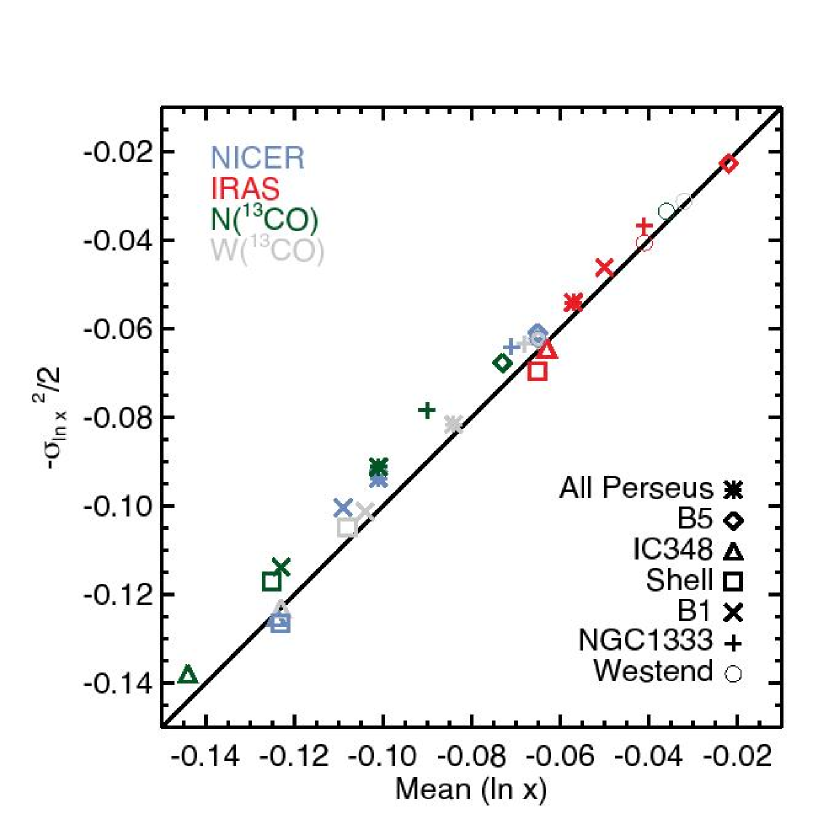
Figure 6.— Comparison of the fit parameters listed in Table 2 with each other, and with the 1:1 line predicted, for a log-normal, by eq. (5).

If a relationship similar to eq. (4) were satisfied, then moving up and right along the “perfect log-normal” line in Figure 6 would mean higher Mach number in the hydrodynamic case, or possibly higher fast magnetosonic Mach number (as shown by Ostriker et al. 2001, in their Figure 4). Note that $\mathcal{M}$ will rise if the sound speed drops, and $\mathcal{M}_{F}$ will rise either if the magnetic field drops or if the sound speed drops, for a given density of material. We have tested whether a sonic Mach number determined from observed line widths and (dust) temperatures listed in Pineda et al. (2008) increases along the 1:1 line in Figure 6, and it does not.

Making comparisons based on Mach numbers calculated using only dust (not gas) temperature and line-of-sight velocity dispersion limits direct observation-simulation comparison in two important ways. First, we simply cannot calculate $\mathcal{M}_{F}$ (as is used in Ostriker et al., 2001), which is likely more relevant than $\mathcal{M}$ in comparisons, because we do not have field strength measurements. Second, in observations, the observed column distribution arises from plane-of-sky compressions, whereas the line widths used to compute Mach number come from the line-of-sight motions only. We consider how one might get around these limitations in the future in §5.4 below.

One important point to take away from observation-simulation comparisons concerns the sometimes-overlooked distinction between volume density and column density distributions. Several simulators have pointed out that the column density distributions we show here will only look the same as the volume density distributions, which are usually predicted to be log-normal, when turbulence is dominated by large-scale motions (e.g. Ostriker et al., 2001) . The fact that the distributions look as close to log-normal as they do suggests that turbulence in Perseus is primarily driven by motions on scales nearly the size of the whole cloud, or larger.

5.2. How common are log-normal-like density distributions?

A similar relationship to the one shown in Figure 6, between the mean and dispersion in column density, has been used to explain and interpret the results of Lada et al. (1994), who we believe were the first to find a relation between the standard deviation in measured extinction and the extinction value itself. Thoraval et al. (1997) pointed out that a relation like eq. (5) can be caused by small scale structure below the resolution limit of an extinction map. Padoan et al. (1997a) performed a reanalysis of Lada et al.’s IC5146 observations, and find that the $\sigma_{A_{V}}-A_{V}$ relation is consistent with a log-normal column density distribution producing unresolved density structure. Later, Ostriker et al. (2001) used higher resolution observation in IC5146 by Lada et al. (1999) to compare the cumulative column density distribution with their own simulations finding that they are very similar in shape.

Other extinction studies might provide notable exceptions to the “log-normal” trend. For example, the Pipe Nebula’s column-density distribution (determined using the 2MASS/NICER method) displays a complex shape with multiple peaks (Lombardi et al., 2006). Lombardi et al. attribute these peaks to the possibility of background clouds observed in projection with (and thus in addition to) the Pipe at low Galactic latitudes. Recent C¹⁸O observations in the Pipe (Muench et al., 2007) have shown that there are two distinct velocity components there, and so it is possible that if those distributions could be separated, each would have a more log-normal-like column density distribution.

In general, it is important to consider what boundaries, in either spatial or velocity dimensions, are placed upon regions when assessing how common log-normal distributions might be. Overlapping “clouds” along the line of sight may appear as one structure on the plane of the sky, and, without kinematic or distance information, it is hard to separate these structures. And, even if one can separate populations along a line of sight, the meaning of the region one considers on the plane of the sky needs to be understood as physically “small” or “large” in the context of a particular question, such as how “log-normal” a distribution might be expected to look.

5.3. Which Tracer Tells us What, how Reliably?

Recently, in a paper entitled “Can We Trust the Dust?”, Padoan et al. (2006) have raised questions about the reliability of NIR extinction mapping, based on their finding that the power spectrum of a NIR extinction map of the Taurus region is significantly shallower than that derived from a ¹³CO map of the same region. Through detailed modelling, they rule out depletion of CO, and/or CO formation timescales as the cause(s) of this discrepancy. By producing synthetic NIR-extinction observations of simulations, they show that the power spectrum derived from observations should trace the power spectrum of the actual spatial distribution of dust if the extinction is proportional to dust column density.

Padoan et al. (2006) argue that a discrepancy between the power spectra of the dust and the gas might be expected in the case of transonic, nonmagnetized turbulence. Using ¹³CO and NIR data as we do here, but for Taurus, they interpret a shallower power spectrum in dust fluctuations than in gas fluctuations as evidence for intrinsic spatial fluctuations in the dust-to-gas ratio, with amplitude increasing toward smaller scales. Strictly, the Padoan et al. (2006) work is only applicable at very small scales (their estimate is $<0.1$ pc). Thus, the apparent disagreement between our results, which show the gas to be less reliable, and theirs which question the veracity of dust as a tracer of column density, may be only a question of scale.

On the other hand, as shown by Pineda et al. (2008) in Perseus, the ¹³CO-dervied column density estimates are adversely effected by optical depth even at $A_{V}\sim 4$ mag, and variation in the ¹³CO abundance with respect to ${\rm H_{2}}$ is found between regions in the same molecular cloud. These caveats in the interpretation of the ¹³CO emission maps are not fully taken into account in the Padoan et al. (2006) analysis (which assumes ¹³CO to trace density faithfully out to $A_{V}\sim 10$ mag), and may also explain the apparent disagreements–both between gas and dust, and between our results and “Can We Trust the Dust?.”

We have clearly demonstrated, in every figure in this paper, that gas-based and dust-based measures of column density almost never agree perfectly in detail. So, instead of “Can We Trust the Dust?”, one might ask instead “Should we Sass the Gas?”. As we discussed in §4.1, dust and gas measures are virtually never tracing exactly the same portions of any particular line of sight, so some amount of “disagreement” when inter-comparing tracers has to be expected. It also has to be recognized, though, that any particular molecular transition can only trace a (sometimes very) limited range of volume densities, which is effectively bounded at bottom by the critical density and at top by depletion and/or opacity. Because it is hard to know the real density range to which a line is sensitive, and to model how linear the conversion from line flux to density is likely to be, gas really does deserve some degree of sassing if one wants to tease its ability to trace column density cleanly.

Dust, however, is not perfect either. For extinction-based measures, variations in the compositional and size distribution of grains can effect the reddening law. And, for emission-based measures, variations in grain temperature along the line of sight are impossible to correct for and so impose unavoidable uncertainty (Schnee et al., 2006).

The principle advantage of Dust over Gas is dynamic range. No single observation of a gas tracer can sample more than about a factor of a about ten in column density, but, dust-based measurements can span a dynamic range of 50 or (much) more. For example, in the famous B68 Globule, observations of extinction span the range $\sim 0$ to 27 mag (Alves et al., 2001) while C¹⁸O ranges from 0.2 to 0.8 K km s^-1 and then depletes, and N₂H⁺, which only is detected above about $A_{V}$ of 10, spans the range 0.3 to 2.1 K km s^-1 (Bergin et al., 2002, Figure 1). In TMC-1C, thermal dust emission allows for a dynamic range of nearly 25 in $A_{V}$  (from 4 to 90 mag, Schnee et al., 2007b), but none of the many lines mapped there has a dynamic range of more than ten (Schnee et al., 2007a).

Extinction measures will always saturate at some high value of extinction where background sources cannot be detected, and emission is often limited in utility at very low extinctions, due to low flux levels and/or observational strategies (e.g. chopping) that make mapping extended emission difficult. In cases where one can can cross-calibrate extinction and emission using maps of regions where they should give the same information, one can stretch the dynamic range of “dust” to its fullest by using extinction as the sole probe at low column densities, emission alone at the higher ones, and both extinction and emission in the intermediate regime.

In the maps of Perseus in this paper, we have excised points with no ¹³CO emission, but our dust measures still can trace low-density material along those lines of sight that do emit in ¹³CO (see §4.1 and Figure 4). In Figure 6 of Schnee et al. (2005) we show the dust-based column density distributions for all of Perseus, without limiting ourselves to ¹³CO-emitting regions. Those distributions look similar to the ones in Figure 2, except that they show a longer high-density tail, caused in large part by not excluding all of the high-density cluster regions NGC1333 and IC348. It is very important to realize that our excision of plane-of-the sky points with no ¹³CO here does not exclude low-column regions traced by dust along the line of sight, which is why the distributions in Figures 2 and 5 look more symmetric (not cut-off at the low end) for the dust measures than for ¹³CO.

The only advantage of Gas over Dust when mapping column density is the ability it offers to kinematically separate regions along the line of sight. Otherwise, Dust wins.

5.4. How to Map Column Density Distributions in the Future?

From the discussion above, we may sound ready to recommend dust as the single best tracer of column density in interstellar space–but we are not. We cannot forget that the total (gas + dust) column density in any region can only be as accurate as the gas-to-dust conversion factor used. And, since all interstellar regions contain much more gas than dust, a small error in a dust-dervied column will be compounded when converted to total column.

Therefore, we recommend a “holistic” approach to measuring column density. We need to take account of the level of uncertainty inherent in each conversion factor (e.g. abundance ratio, reddening-to-extinction ratio, dust opacity, dust-to-gas ratio) and assumption (e.g. about line of sight structure) we use in a column density calculation, and then we need to choose the best solution for each particular question. For example, in a circumstance where we are relatively confident that the dust-to-gas ratio is not varying, and that line-of-sight blending is not causing confusion, then extinction maps will provide the best handle on the kind of relative column density measurements needed to measure key distribution functions, such as “clump” mass functions. On the other hand, in a region where the dust-to-gas ratio is very uncertain (e.g. near an HII region) using molecular line ratios to measure volume density and opacity and converting to column density may be superior. In other words, we recommend that more care than has been typical in the past be given to making the most appropriate choice in any particular study.

Lastly, several recent studies have shown that “observing” simulations using radiative transfer and/or chemistry codes, and synthetic telescopes that mimic biases imposed by real ones (an approach we have called “Taste-Testing”) can sometimes uncover hidden limitations and biases associated with certain techniques (e.g. Schnee et al., 2006; Padoan et al., 2006). Thus, if a realistic simulation can be observed synthetically with various column density probes, it can provide a good guide to which kind(s) of column density measures might be least biased under relevant conditions.

5.5. Conclusions

Careful re-calibration and inter-comparison of extinction, thermal emission, and molecular emission maps of Perseus has allowed us to conclude that:

• The column density distribution of material in the full Perseus star-forming region, with $1<A_{V}<12$ mag, is roughly log-normal, when it is not directly effected by embedded clusters or young stellar outlows (bipolar or spherical).

• Dust is superior to molecular lines for tracing out the “full” mass distribution over the range of extinction studied, because it does not require a threshold density to “excite” and it does not die out at high densities due to high opacity or chemical depletion, the way ¹³CO does.

• The dearth of molecular gas (¹³CO) in the region corresponding the shell created by the B-star HD 278942 suggests that either CO has not yet formed in this young structure, and/or that existing molecular gas has been dissociated by the shell’s interaction with the cloud.

• When Perseus is dissected into smaller “sub-regions,” the column density distributions become more ragged, as is predicted by simulations for samples that are statistically small. However, we find that the sub-regions distributions are still log-normal-like, in that the relationship between their normalized means and their dispersions follows a trend consistent with log-normal distribution.

• In comparing observations of column density (or mass) distributions with each other, and/or with simulations, it is perhaps more important than has been previously appreciated to account for the effects of biases due to dust temperature variations, abundance variations, opacity effects, and observing strategies.

We recommend, for the near-term future, the assemblage of an ensemble of maps of column density, along with measurements of Mach number and magnetic field strength, in order to assess the turbulent properties of molecular clouds and star-forming regions more generally. This large sample is needed to allow for legitimate comparisons between regions, and of observations with simulations, because any one observation of even the same turbulent flow is not enough to characterize the flow’s statistical nature. With such a large sample, we could carry out much more discriminating comparative analyses than the kind represented by Figure 6, which focuses only on testing whether the conditions relating the mean (first moment) of a distribution to its width (second moment) are correct. We could, for example, begin to investigate the skewess of these distributions, and to investigate alternative functional forms, which may in fact not be exactly log-normal. With this larger sample, we could also study the effects of star-formation as a driver of the turbulence, and again compare with simulations of this process.

The combination of: 1) extensive recent improvements in extinction mapping made possible by large-scale near-infrared surveys; 2) the advent of huge molecular line surveys of relatively high-density tracers; and 3) increases in polarization mapping speed (which leads to Chandrasekhar-Fermi-based field estimates), should very soon allow for studies large enough to test predictive theories and simulations of molecular cloud topology using unprecedentedly large observational statistical samples, and we look forward to it.

References

- Alves et al. (2001) Alves, J. F., Lada, C. J., & Lada, E. A. 2001, Nature, 409, 159
- Arce & Goodman (2001) Arce, H. G., & Goodman, A. A. 2001, ApJ, 551, L171
- Bachiller & Cernicharo (1986) Bachiller, R., & Cernicharo, J. 1986, A&A, 166, 283
- Barnard (1927) Barnard, E. 1927, A Photographic Atlas of Selected Regions of the Milky Way, ed. E. Frost & M. Calvert (Carnegie Institute of Washington)
- Bergin et al. (2002) Bergin, E. A., Alves, J., Huard, T., & Lada, C. J. 2002, ApJ, 570, L101
- Bohlin et al. (1978) Bohlin, R. C., Savage, B. D., & Drake, J. F. 1978, ApJ, 224, 132
- Cambrésy (1999) Cambrésy, L. 1999, A&A, 345, 965
- Caselli et al. (1999) Caselli, P., Walmsley, C. M., Tafalla, M., Dore, L., & Myers, P. C. 1999, ApJ, 523, L165
- Cernicharo & Bachiller (1984) Cernicharo, J., & Bachiller, R. 1984, A&AS, 58, 327
- Cernicharo et al. (1985) Cernicharo, J., Bachiller, R., & Duvert, G. 1985, A&A, 149, 273
- Draine (2003) Draine, B. T. 2003, ARA&A, 41, 241
- Enoch et al. (2006) Enoch, M. L., et al. 2006, ApJ, 638, 293
- Evans et al. (2003) Evans, N. J., II, et al. 2003, PASP, 115, 965
- Foster et al. (2008) Foster, J. B., Román-Zúñiga, C. G., Goodman, A. A., Lada, E. A., & Alves, J. 2008, ApJ, 674, 831
- Goodman et al. (1995) Goodman, A. A., Jones, T. J., Lada, E. A., & Myers, P. C. 1995, ApJ, 448, 748
- Goodman et al. (2008) Goodman, A., Rosolowsky, E., Borkin, M., Foster, J., Halle, M., Kauffmann, J., & Pineda, J. E. 2008, Nature, submitted
- Hirota et al. (2008) Hirota, T., et al. 2008, PASJ, 60, 37
- Jørgensen et al. (2006) Jørgensen, J. K., et al. 2006, ApJ, 645, 1246
- Kirk et al. (2006) Kirk, H., Johnstone, D., & Di Francesco, J. 2006, ApJ, 646, 1009
- Lada et al. (1994) Lada, C. J., Lada, E. A., Clemens, D. P., & Bally, J. 1994, ApJ, 429, 694
- Lada et al. (1999) Lada, C. J., Alves, J., & Lada, E. A. 1999, ApJ, 512, 250
- Langer et al. (1989) Langer, W. D., Wilson, R. W., Goldsmith, P. F., & Beichman, C. A. 1989, ApJ, 337, 355
- Lombardi & Alves (2001) Lombardi, M., & Alves, J. 2001, A&A, 377, 1023
- Lombardi et al. (2006) Lombardi, M., Alves, J., & Lada, C. J. 2006, A&A, 454, 781
- Miville-Deschênes & Lagache (2005) Miville-Deschênes, M.-A., & Lagache, G. 2005, ApJS, 157, 302
- Muench et al. (2007) Muench, A. A., Lada, C. J., Rathborne, J. M., Alves, J. F., & Lombardi, M. 2007, ApJ, 671, 1820
- Nordlund & Padoan (1999) Nordlund, Å. K., & Padoan, P. 1999, Interstellar Turbulence, 218
- Onishi et al. (1999) Onishi, T., et al. 1999, PASJ, 51, 871
- Ostriker et al. (2001) Ostriker, E. C., Stone, J. M., & Gammie, C. F. 2001, ApJ, 546, 980
- Padoan et al. (1997a) Padoan, P., Jones, B. J. T., & Nordlund, A. P. 1997, ApJ, 474, 730
- Padoan et al. (1997b) Padoan, P., Nordlund, A., & Jones, B. J. T. 1997, MNRAS, 288, 145
- Padoan et al. (1999) Padoan, P., Bally, J., Billawala, Y., Juvela, M., & Nordlund, Å. 1999, ApJ, 525, 318
- Padoan et al. (2006) Padoan, P., Cambrésy, L., Juvela, M., Kritsuk, A., Langer, W. D., & Norman, M. L. 2006, ApJ, 649, 807
- Pineda et al. (2008) Pineda, J. E.., Caselli, P. & Goodman, A. A. 2008, ApJ, 679, 481
- Ridge et al. (2006a) Ridge, N. A., et al. 2006, AJ, 131, 2921
- Ridge et al. (2006b) Ridge, N. A., Schnee, S. L., Goodman, A. A., & Foster, J. B. 2006, ApJ, 643, 932
- Rosolowsky et al. (2008) Rosolowsky, E., Pineda, J. E.., Kauffmann, J., & Goodman, A. A. 2008, ApJ, 679, 1338
- Schlegel et al. (1998) Schlegel, D. J., Finkbeiner, D. P., & Davis, M. 1998, ApJ, 500, 525
- Schnee et al. (2005) Schnee, S. L., Ridge, N. A., Goodman, A. A., & Li, J. G. 2005, ApJ, 634, 442
- Schnee et al. (2006) Schnee, S., Bethell, T., & Goodman, A. 2006, ApJ, 640, L47
- Schnee et al. (2007a) Schnee, S., Caselli, P., Goodman, A., Arce, H. G., Ballesteros-Paredes, J., & Kuchibhotla, K. 2007, ApJ, 671, 1839
- Schnee et al. (2007b) Schnee, S., Kauffmann, J., Goodman, A., & Bertoldi, F. 2007, ApJ, 657, 838
- Schnee et al. (2008) Schnee, S., Li, J., Goodman, A. A., & Sargent, A. I. 2008, ApJ, 684, 1228
- Thoraval et al. (1997) Thoraval, S., Boisse, P., & Duvert, G. 1997, A&A, 319, 948
- Vázquez-Semadeni (1994) Vázquez-Semadeni, E. 1994, ApJ, 423, 681