Non-equilibrium processes: driven lattice gases, interface dynamics, and quenched disorder effects on density profiles and currents

Abstract

Properties of the one-dimensional totally asymmetric simple exclusion process (TASEP), and their connection with the dynamical scaling of moving interfaces described by a Kardar-Parisi-Zhang (KPZ) equation are investigated. With periodic boundary conditions, scaling of interface widths (the latter defined via a discrete occupation-number-to-height mapping), gives the exponents $\alpha=0.500(5)$, $z=1.52(3)$, $\beta=0.33(1)$. With open boundaries, results are as follows: (i) in the maximal-current phase, the exponents are the same as for the periodic case, and in agreement with recent Bethe ansatz results; (ii) in the low-density phase, curve collapse can be found to a rather good extent, with $\alpha=0.497(3)$, $z=1.20(5)$, $\beta=0.41(2)$, which is apparently at variance with the Bethe ansatz prediction $z=0$; (iii) on the coexistence line between low- and high- density phases, $\alpha=0.99(1)$, $z=2.10(5)$, $\beta=0.47(2)$, in relatively good agreement with the Bethe ansatz prediction $z=2$. From a mean-field continuum formulation, a characteristic relaxation time, related to kinematic-wave propagation and having an effective exponent $z^{\prime}=1$, is shown to be the limiting slow process for the low density phase, which accounts for the above-mentioned discrepancy with Bethe ansatz results. For TASEP with quenched bond disorder, interface width scaling gives $\alpha=1.05(5)$, $z=1.7(1)$, $\beta=0.62(7)$. From a direct analytic approach to steady-state properties of TASEP with quenched disorder, closed-form expressions for the piecewise shape of averaged density profiles are given, as well as rather restrictive bounds on currents. All these are substantiated in numerical simulations.

I Introduction

In the absence, so far, of a general theory describing non-equilibrium processes (even in steady state), it is worthwhile studying simple models whose qualitative features, it is hoped, will hold for a broad class of systems. In this paper we deal with properties of the one-dimensional totally asymmetric simple exclusion process (TASEP) derr98 , and their connection with the dynamical scaling of moving interfaces described by a Kardar-Parisi-Zhang (KPZ) equation kpz ; hhz95 ; bar95 . The TASEP is a biased diffusion process for particles with hard-core repulsion (excluded volume) derr98 ; sch00 ; derr93 .

Our main purpose is twofold: first, to probe the relationship between TASEP behavior and KPZ interface evolution under several distinct constraints, to be described below; and, focusing especifically on systems with quenched disorder, to provide an account of the effects of frozen randomness on the density profiles and currents in TASEP.

Upon implementing specific features on the particle system, such as various boundary conditions, assorted particle densities, currents, and/or injection/ejection rates, as well as quenched inhomogeneities, we measure the consequent changes to properties of the interface problem, taking the latter to be related to the former by the connection which we now sketch.

The $1+1$ dimensional TASEP is the fundamental discrete model for flow with exclusion. Here the particle number $n_{\ell}$ at lattice site $\ell$ can be $0$ or $1$, and the forward hopping of particles is only to an empty adjacent site. Taking the stochastic attempt rate $p=1$ (see later) the current across the bond from $\ell$ to $\ell+1$ is thus $J_{\ell,\ell+1}=n_{\ell}(1-n_{\ell+1})$. This system maps exactly to an interface growth model meakin86 in $D=1+1$, having integer values of height variables $h_{i(\ell)}$ on a new lattice such that $i(\ell)$ lies midway between sites $\ell$, $\ell+1$ of the TASEP lattice. The $h_{i}$ are constrained by the relation $h_{i(\ell+1)}-h_{i(\ell)}=1-2\,n_{\ell}$ ($=\pm 1$). When not concerned with detailed associations of sites between the models we will omit the $(\ell)$ in $i(\ell)$; after continuum limits, $(\ell)$ and $i(\ell)$ become the same.

There is clearly a precise one-to-one correspondence between these two discrete models and their stochasticity. Various associated continuum models are not so clearly related, due to the possibility of different continuum limits. A naive continuum limit in the TASEP gives ks91 ; kk08 the noisy Burgers turbulence equation ks91 ; fns77 ; vBks85 for one-dimensional particle flow: this equation is the continuity equation resulting from a continuum version of the TASEP bond current $J$, which takes the form

$$J=-\frac{1}{2}\frac{\partial\rho}{\partial x}-\left(\rho-\frac{1}{2}\right)^{2}+\zeta(x,t)+\frac{1}{4}\ ,$$ (1)

where $\rho=\langle n\rangle$ (i.e., the "mean field" version of $n$), and $\zeta(x,t)$ is the (uncorrelated) noise here used to represent all the effects of stochasticity: $\langle\zeta(x,t)\,\zeta(x^{\prime},t^{\prime})\rangle=\delta(x-x^{\prime})\,\delta(t-t^{\prime})$.

Using the continuum "noiseless" version of the height/occupation given above for the discrete models, i.e.,

$$\frac{\partial h}{\partial x}=1-2\rho\ ,$$ (2)

it is seen that the Burgers equation is related by a spatial derivative to the KPZ equation kpz for the evolution of the height $h(x,t)$ of an elastic interface above a fixed reference level:

$$\frac{\partial h}{\partial t}=\frac{\partial^{2}h}{\partial x^{2}}+\left(\frac{\partial h}{\partial x}\right)^{2}+\zeta(x,t)\ .$$ (3)

Depending on boundary conditions imposed at the extremities, one can have different regimes for the TASEP derr98 ; derr93 , whose features will be recalled below where pertinent. There should be corresponding regimes also for KPZ, as pointed out previously mukamel ; kgmd93 .

In Section II we investigate the TASEP with periodic boundary conditions, and the associated interface problem. By examination of interface width scaling, we estimate the respective critical exponents. We also study the behavior of asymptotic interface widths against particle density in the TASEP, as well as the main features of interface slope distributions and their connections to TASEP properties. In Sec. III, we examine the interface width evolution corresponding to open-boundary TASEP systems in the following phases: (i) maximal-current, (ii) low-density, and (iii) on the coexistence line. In the latter case, we also calculate density profiles in the particle system. In Sec. IV we turn to quenched bond disorder in the TASEP with PBC, providing a scaling analysis of the associated interface widths, as well as results for interface slope distributions. A direct analytic approach to steady-state properties of the TASEP with quenched disorder is given, focusing on averaged profiles densities and system-wide currents. Finally, in Sec. V, concluding remarks are made.

II Periodic boundary conditions

We start by imposing periodic boundary conditions (PBC) for the TASEP at the ends of the chain, thus the total number of particles is fixed. Henceforth, the position-averaged particle density $\langle\rho\rangle$ will be denoted simply by $\rho$. Several steady-state properties are known exactly in this case derr98 , as the configuration weights are factorizable at stationarity. To make contact with KPZ interface properties, we consider the width $w(L,t)$ of an evolving interface of transverse size $L$ in $1+1$ dimensions in the discrete height model outlined in Section I. The average interface slope is $1-2\rho$ [ see Eq. (2) ], and this average tilt must be taken into account. This is done by defining

$$\left[w(L,t)\right]^{2}=L^{-1}\,\sum_{i=1}^{L}\left(h_{i}(t)-{h_{1}}(t)-(1-2\rho)\,(i-1)\right)^{2}\ ,$$ (4)

where only fluctuations around the baseline trend are considered. Initially, $w$ grows with time as $t^{\beta}$, until a limiting, $L$-dependent width $\sim L^{\alpha}$ is asymptotically reached. With $z=\alpha/\beta$, one expects from scaling bar95 ; hhz95 :

$$w(L,t)=L^{\alpha}\,f\left(\frac{t}{L^{z}}\right)\ ,$$ (5)

where

$$f(u)=\begin{cases}{u^{\beta}\quad u\ll 1}\cr{{\rm const.}\quad u\gg 1\ .}\end{cases}$$ (6)

For the $D=1+1$ KPZ model, one has the exact values kpz : $\alpha=1/2$, $\beta=1/3$, $z=3/2$.

We have simulated the TASEP on lattices with $L=325$, $650$, and $1300$ sites with PBC. For specified densities $\rho$, we would start from a particle configuration as uniform as possible, in order to minimize the associated interface width. A time step is defined as a set of $L$ sequential update attempts, each of these according to the following rules: (1) select a site at random, and (2) if the chosen site is occupied and its neighbor to the right is empty, move the particle. Thus, the stochastic character resides exclusively in the site selection process. At the end of each time step we measured the width of the corresponding interface configuration. We took typically $N_{s}=10^{4}$ independent runs, averaging the respective results for each $t$. The evolution of interface widths for $\rho=1/2$ and assorted lattice sizes is shown in Fig. 1; the goodness of their scaling with the exact KPZ indices is typical of what is attained over the full density range. By examining the variation of data collapse quality against changes in the fitting exponents, we estimate $\alpha=0.500(5)$, $z=1.52(3)$ for $\rho=1/2$. Direct measurement of the short-time exponent $\beta$ is less accurate; for example, fitting the $L=1300$ data of Fig. 1 for $10^{2}<t<10^{3}$ to a single power law gives $\beta=0.31(1)$.

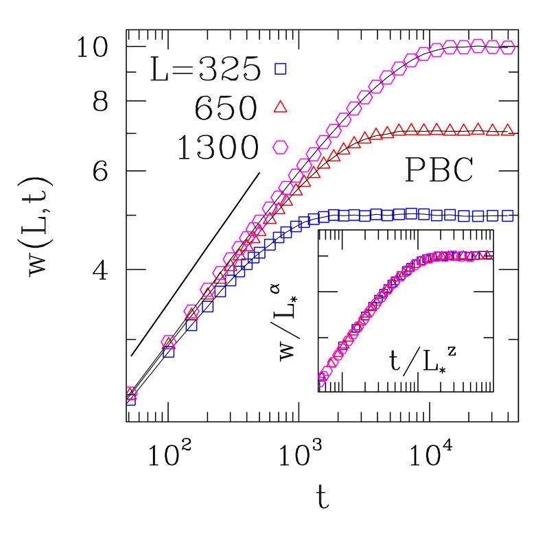
Figure 1: (Color online) Double-logarithmic plot of interface width against time, corresponding to TASEP with periodic boundary conditions, $\rho=1/2$, lattice sizes $L$ as in key to symbols. Full line corresponds to $w\sim t^{1/3}$. Inset: scaling plot of data on main diagram, using $\alpha=1/2$, $z=3/2$; $L_{\ast}=L/325$.

The limiting (asymptotic) interface width, $w_{\rm lim}$ obeys the $\rho\leftrightarrow 1-\rho$ particle-hole symmetry of the TASEP, with a maximum at $\rho=1/2$. Fig. 2 exhibits the behavior of $w_{\rm lim}$ for $\rho\leq 1/2$, and lattice size $L=325$. The leftmost data point corresponds to eight particles, i.e. $\rho=0.0246$. For even lower densities, discrete-lattice effects become more prominent, and the time needed to attain asymptotic behavior increases significantly.

From Eq. (4), using $h_{i}-h_{i-1}=1-2n_{i-1}$, the squared width is

$$\left[w(L,t)\right]^{2}=\frac{4}{L}\,\sum_{i=1}^{L}\left\{(i-1)\rho-\sum_{m=1}^{i-1}n_{m}\,\right\}^{2}\ .$$ (7)

For the steady state with PBC, the configurational weights are factorizable derr98 : each $n_{m}$ is independently distributed, taking values $(0,1)$ with probabilities $(\rho,1-\rho)$. Consequently, in this case the average of $\left[(i-1)\rho-\sum_{m=1}^{i-1}n_{m}\,\right]^{2}$ is $(i-1)(\rho-\rho^{2})$, and the steady state rms width is

$$\left[\langle w(L)^{2}\rangle\right]^{1/2}=c\,(L-1)^{1/2}\,[\rho(1-\rho)]^{1/2}\ ,$$ (8)

where $c$ is a numerical constant. This form, consistent with having the KPZ scaling exponent $\alpha=1/2$, is compared with the simulation results for averaged limiting widths in Fig. 2.

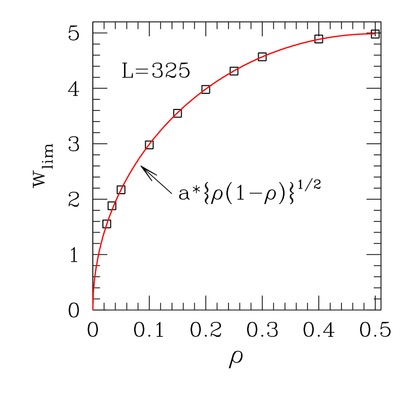
Figure 2: (Color online) Limiting interface width $w_{\rm lim}$ against particle density $\rho$ for lattice with $L=325$, PBC. Squares are numerical results, from $N_{s}=10^{4}$ samples each. Error bars are smaller than symbol sizes. The full line is the analytic expression, Eq. (8), with $a=9.97$ (see text).

According to Eq. (2), particle density fluctuations can be investigated via the probability distribution functions (PDF) for slopes of the associated interface problem. In doing so within the context of a discrete-lattice model, one must take recourse to a coarse-grained description. We have experimented by taking interface segments with a varying number $m$ of bonds, and calculating the average slopes between the respective endpoints. For $m\gtrsim 10$ (the smallest practicable limit, such that the discreteness of allowed slope values still permits one to speak of a relatively smooth PDF), the curves are very close to Gaussians, and their width (height at peak) varies with $m$ as $m^{-1/2}$ ($m^{1/2}$).

This can be understood by recalling the specific form of the (factorizable) particle configuration weigths in this case derr98 . Taking $\rho$ as the overall density, the probability of occurrence of a configuration with average slope $s=1-2x$ (i.e., average local density $x\in[0,1]$), on a lattice section with $m$ sites is

$$P(x)\sim C_{m}^{mx}\,\rho^{mx}\,(1-\rho)^{m(1-x)}\ .$$ (9)

Standard treatment of Eq. (9) shows that, close to the maximum at $x=\rho$, the curve shape is indeed Gaussian, with a width proportional to $m^{-1/2}$.

Having thus established the nature of the $m$-dependence of slope PDFs, we have used $m=60$ in our calculations, which gives a convenient, almost continuous, spectrum of allowed slopes. Results for the stationary state are depicted in Fig. 3. One sees that the $\rho=0.5$ PDF is fitted by a Gaussian down to some four orders of magnitude below the peak, while for $\rho=0.2$, departures from a Gaussian profile are noticeable already at PDF values $\sim 10^{-2}$ times those at the maximum.

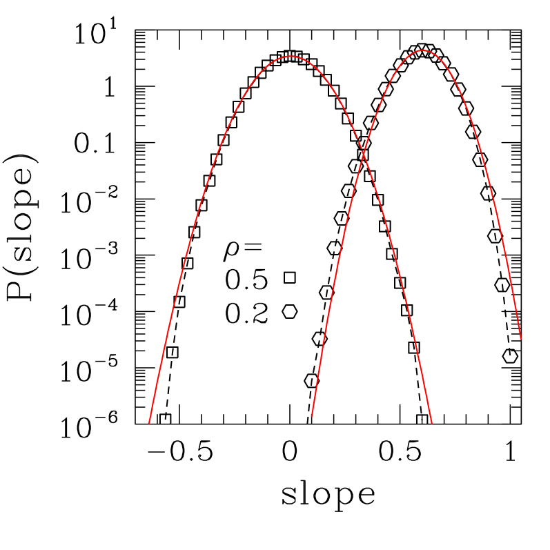
Figure 3: (Color online) Slope PDFs in stationary state, lattice size $L=325$ with PBC, for $\rho=1/2$ and $0.2$. Full lines are Gaussian fits to data.

We have followed the evolution of interface slope PDFs during the transient regime (starting from a particle distribution as uniform as possible), for $\rho=1/2$. We ascertained that, already from early times, their shapes are very well approximated by Gaussians. Fig. 4 shows the (root-mean-square) widths of Gaussian fits to the PDFs against time.

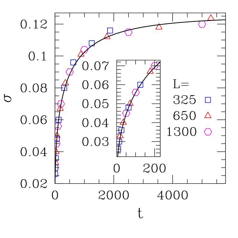
Figure 4: (Color online) Width $\sigma$ of slope distributions in transient regime against time, for $\rho=1/2$ and assorted lattice sizes $L$ with PBC. Initial particle configuration: alternate empty and filled sites, for minimum interface width. Full line is stretched exponential fit to data (see text). Inset shows details of main figure, close to the vertical axis.

It is noteworthy that, contrary to the behavior of interface widths shown in Fig. 1, here one does not find any significant dependence on lattice size. It thus appears that, even during the transient, the range of density fluctuations for $\rho=1/2$ is shorter than the smallest lattice size considered here, $L=325$. The solid curve in Fig. 4 is a stretched exponential, $F(t)=a-b\,\exp\left\{-(t/t_{0})^{\delta}\right\}$, for which the best-fitting parameter values are $t_{0}=380(20)$, $\delta=0.51(2)$.

In summary, we have shown that our methods, namely inferring scaling properties of TASEP via those of the associated interface problem, do give rather accurate results (where comparison is possible, i.e., for the scaling exponents $\alpha$, $\beta$, and $z$) in the simplest case of a purely stochastic system with PBC. Our results so far are in agreement with the so-called KPZ conjecture kk08 , sketched in Eqs. (1)-(3) above.

III Open boundary conditions

III.1 Numerical results

With open boundary conditions, the following additional quantities are introduced: the injection rate $\alpha_{I}$ at the left end, and the ejection rate $\beta_{E}$ at the right one (both defined as fractions of the internal hopping rate). The number of particles is no longer constant, although at stationarity it fluctuates around a well-defined average. Therefore, in order to consider the associated interface widths, one needs to subtract the instantaneous average slope $1-2\rho(t)$, in the manner of Eq. (4), at each time step.

Many stationary properties are known for this case derr98 ; sch00 ; derr93 ; ds04 ; rbs01 ; be07 , including the phase diagram in $(\alpha_{I},\beta_{E})$ space. With open boundary conditions one must be aware that, even at stationarity, ensemble-averaged quantities such as densities will locally deviate from their bulk values, within "healing" distances from the chain extremities which depend on the boundary (injection/ejection) rates.

Numerical density-matrix renormalization group (DMRG) techniques have been applied to estimate the dynamic exponent $z$ for several locations on the phase diagram nas02 . More recently ess05 , a Bethe-ansatz solution has been provided, giving exact (analytic) predictions for the value of $z$ everywhere on the phase diagram.

We started by investigating the maximal-current (MC) phase ($J=1/4$) at $\alpha_{I}>1/2$, $\beta_{E}>1/2$. The Bethe ansatz solution ess05 predicts the KPZ value $z=3/2$ there, concurrently with DMRG results nas02 . We took $\alpha_{I}=\beta_{E}=3/4$, starting from an initial configuration with $\rho=1/2$ (in the present case, this is the average final density as well), and alternate empty and filled sites, for minimum interface width. The evolution of interface widths against time was very similar to the PBC case, as shown in Fig. 5, and the KPZ exponents $\alpha=1/2$, $\beta=1/3$, $z=3/2$ were extracted within error bars of the same order as those for PBC. We also checked the multicritical point $\alpha_{I}=\beta_{E}=1/2$, and found the KPZ exponents again there, with an accuracy similar to that obtained deep within the MC phase. The value $z=3/2$ has been found at this point by DMRG as well nas02 .

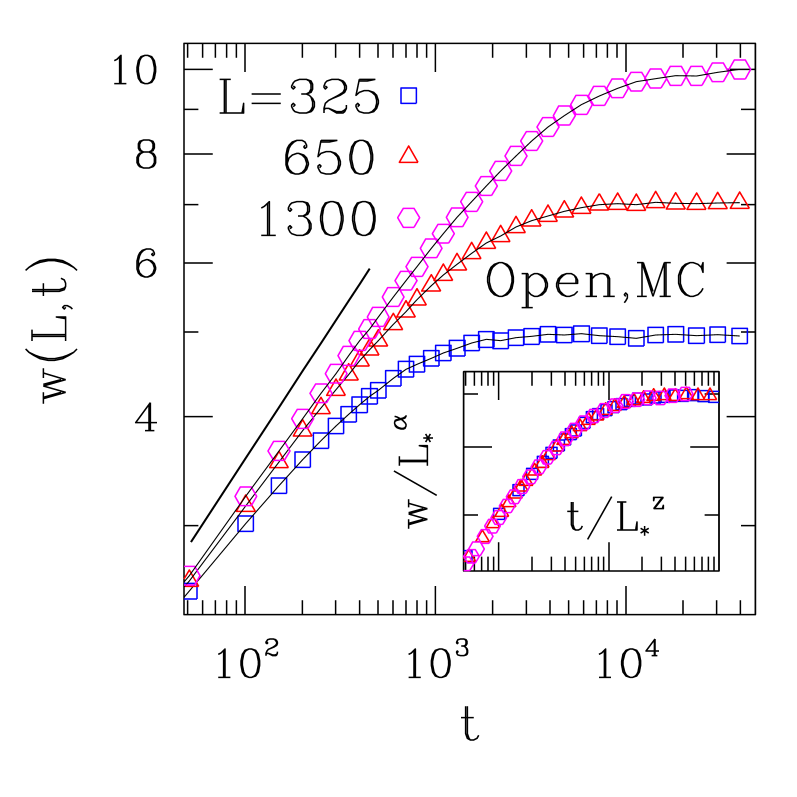
Figure 5: (Color online) Double-logarithmic plot of interface width against time, corresponding to TASEP with open boundary conditions inside the maximal current (MC) phase, $\alpha_{I}=\beta_{E}=3/4$. Initial density $\rho=1/2$, lattice sizes $L$ as in key to symbols. Full line corresponds to $w\sim t^{1/3}$. Inset: scaling plot of data on main diagram, using $\alpha=1/2$, $z=3/2$; $L_{\ast}=L/325$.

Elsewhere on the phase diagram, a low-density phase exists at $\alpha_{I}<1/2$, $\alpha_{I}<\beta_{E}$ (with $\rho=\alpha_{I}$), and a high-density phase at $\beta_{E}<1/2$, $\beta_{E}<\alpha_{I}$ (with $\rho=1-\beta_{E}$) derr98 ; sch00 ; derr93 ; ds04 . There is a critical coexistence line $\alpha_{I}=\beta_{E}<1/2$, where a first-order transition occurs derr98 . The low- and high-density phases are further subdivided ess05 . However, such subdivisions will not concern us directly here, the relevant fact being that (outside the MC phase) the Bethe ansatz solution predicts a non-vanishing gap as $L\to\infty$ (i.e. $z=0$) everywhere (this is found by DMRG as well nas02 ), except on the coexistence line where diffusive behavior with $z=2$ is expected ess05 .

We first examined a point away from the coexistence line, namely $\alpha_{I}=1/4$, $\beta_{E}=1/2$ where the stationary density is thus $\rho=1/4$. Setting the initial density at the stationary value, the time evolution of the associated interface widths is qualitatively very similar to the cases illustrated earlier, as shown in Fig. 6; however, scaling turns out to be very different.

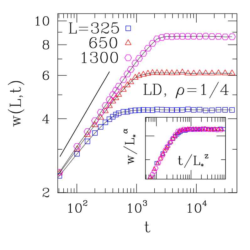
Figure 6: (Color online) Double-logarithmic plot of interface width against time, corresponding to TASEP with open boundary conditions inside the low-density (LD) phase, $\alpha_{I}=1/4$, $\beta_{E}=1/2$. Initial density $\rho=1/4$, lattice sizes $L$ as in key to symbols. Full line corresponds to $w\sim t^{5/12}$. Inset: scaling plot of data on main diagram, using $\alpha=1/2$, $z=6/5$; $L_{\ast}=L/325$.

Attempting curve collapse on the data of Fig. 6 (see inset) gives the following estimates: $\alpha=0.497(3)$, $z=1.20(5)$. This would imply $\beta=0.41(2)$ from scaling; a direct fit of $L=1300$ data for $10^{2}<t<10^{3}$ gives $\beta=0.35(1)$, which is a larger discrepancy compared with the scaling prediction than, e.g., for PBC or for the MC phase with open boundaries.

These results for $\alpha$ and $z$ are inconsistent with the scaling relation $\alpha+z=2$ from galilean invariance kpz ; however, it should be recalled that translational invariance, the key ingredient for galilean invariance to hold, is in general broken by the system’s boundaries here present. The fact that $\alpha+z=2$ is obeyed for open boundary conditions, in the MC phase $\alpha_{I}$, $\beta_{E}\geq 1/2$, can be explained on the basis of simple kinematic-wave theory be07 for the TASEP. Indeed, in this phase the kinematic waves produced by both boundaries do not penetrate the system be07 , and one does not see the formation of a shock (density wave) in the bulk which would otherwise disrupt the translational symmetry.

As mentioned above, both DMRG numerics nas02 and the Bethe ansatz solution ess05 predict $z=0$, i.e., the correlation length is supposed to be finite here. We defer discussion, and a proposed solution, of the apparent contradiction between our own results and previous ones, to Subsection III.2 below, where a continuum mean-field treatment of the approach to stationarity is developed. For the moment, we note that an explanation can be provided for the limiting-width exponent $\alpha$, by going back to Eq. (7) which was there applied to the factorizable-weight case of PBC. As seen from the development immediately below Eq. (7), the only changes brought about by a finite correlation length (assumed to be $\ll L$) amount to an $L$-independent correction to the term within round brackets, resulting from short-range density-density correlations. Thus, the $L^{1/2}$ dependence of $\left[\langle w(L)^{2}\rangle\right]^{1/2}$, given in Eq. (8), remains valid here. This is corroborated by our numerical estimate $\alpha=0.497(3)$, quoted above.

Next, we looked at a point with $\alpha_{I}=\beta_{E}=1/4$, on the coexistence line. In the stationary state, one expects a low-density phase with $\rho_{-}=\alpha_{I}$, and a high-density one with $\rho_{+}=1-\beta_{E}$, to coexist. We investigated the time evolution of both interface widths and overall densities, with two different initial conditions, namely $\rho_{0}=1/4$, $1/2$ (because of particle-hole symmetry, starting with $\rho=3/4$ gives the same interface width as for $\rho=1/4$, and a complementary particle density). It can be seen in Fig. 7 that with both initial conditions, the fixed point for the average density is $\rho=1/2$. While, for $\rho_{0}=1/4$, the time evolution of the associated interface width still displays the simple, monotonic, character found in all setups previously studied here (apart from a small bump at early times), such a feature is lost for $\rho_{0}=1/2$. Though the width eventually settles at a unique saturation value, the corresponding relaxation time is one order of magnitude longer than elsewhere on the phase diagram or for PBC (see the curves for $L=325$ in the respective figures).

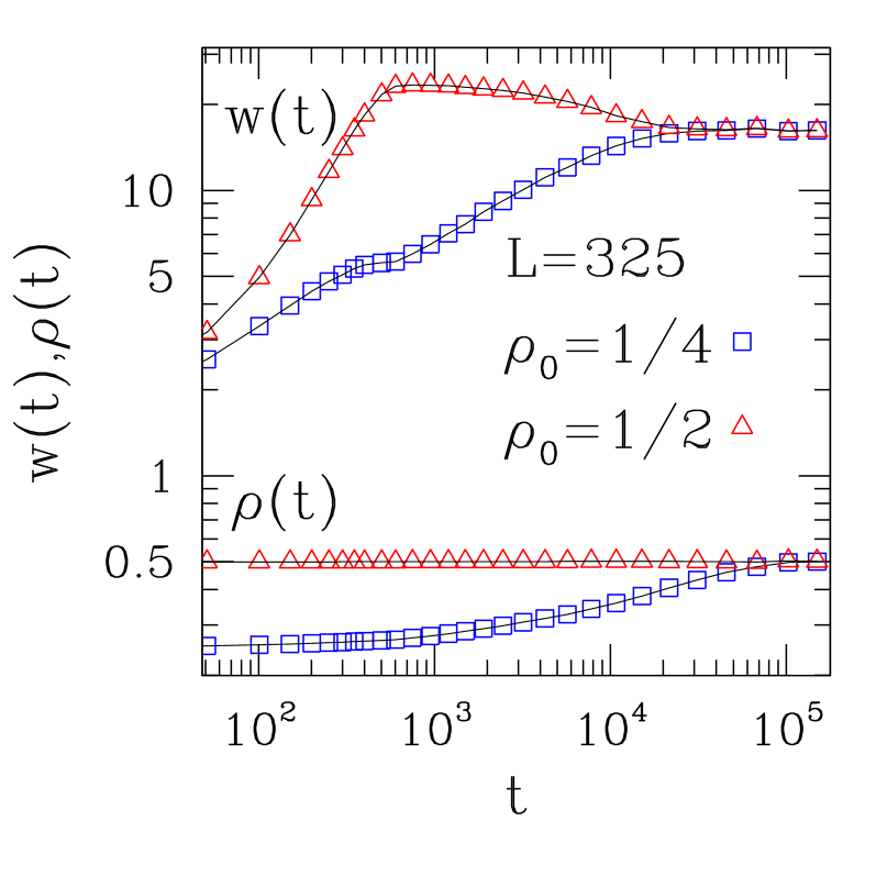
Figure 7: (Color online) Double-logarithmic plot of interface width $w$ and overall particle density $\rho$ against time, corresponding to TASEP with open boundary conditions, at $\alpha_{I}=\beta_{E}=1/4$ (on the coexistence line), lattice size $L=325$, and two distinct initial densities, $\rho_{0}=1/4$ and $1/2$.

In order to unravel the corresponding spatial particle distributions, we also looked at the time evolution of slope PDFs at this point, for the same initial densities.

Results are depicted in Fig. 8, showing that for both cases a double-peaked structure eventually evolves. The peak heights indicate a large degree of spatial segregation between the $\rho_{0}=1/4$ and $3/4$ phases. For example, in case (b) [initial density $\rho_{0}=1/2$], at $t=20000$ the peaks associated to the coexisting densities are $\sim 8$ times higher than the trough in the PDF at slope zero ($\rho=1/2$).

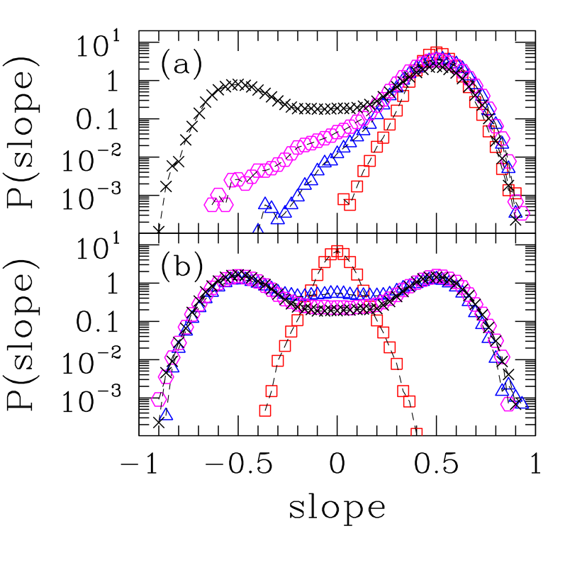
Figure 8: (Color online) Slope PDFs at assorted times, for interfaces corresponding to TASEP with open boundary conditions, at $\alpha_{I}=\beta_{E}=1/4$ (on the coexistence line), lattice size $L=325$, and two distinct initial densities, namely (a) $\rho_{0}=1/4$, and (b) $\rho_{0}=1/2$. Key to symbols: squares, $t=150$ (a), $t=50$ (b); triangles, $t=500$; hexagons, $t=5000$; crosses, $t=20000$.

We pursued this point further, via direct examination of the evolution of averaged density profiles in the particle system. Results for $L=325$, with initial density $\rho_{0}=1/2$ and initial distribution as uniform as possible (i.e., alternating empty and occupied sites), are shown in Fig. 9.

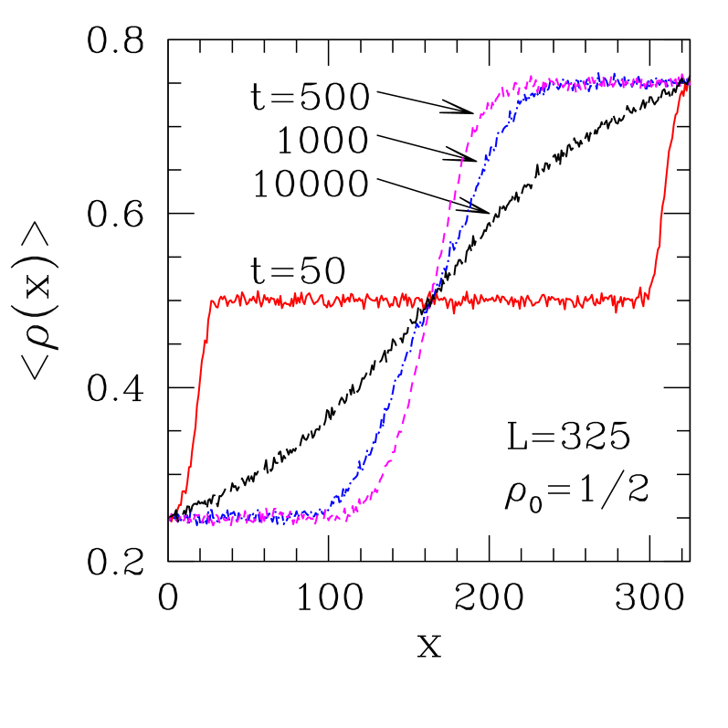
Figure 9: (Color online) Ensemble-averaged particle density profiles at assorted times, for TASEP with open boundary conditions, at $\alpha_{I}=\beta_{E}=1/4$ (on the coexistence line), lattice size $L=325$, and initial density $\rho_{0}=1/2$. Averages taken over $10^{4}$ independent samples (see text).

For $t\lesssim 500$, the low injection/ejection rates cause the the initial plateau of uniform density to be symmetrically eaten into, as illustrated by the $t=50$ profile. After the two density waves meet, a shock (kinematic wave) is formed, which for this case of $\alpha_{I}=\beta_{E}<1/2$, is stationary on average be07 , i.e., it jiggles around and is in effect bounced off the system’s boundaries. For the ensemble-averaged densities at fixed times $\gtrsim 500$, the consequence of this is that the promediated profiles grow ever more featureless (because the spread between locations of the shock, at the same time but for different noise realizations, increases with time owing to increasing sample-to-sample decorrelation). At $t=10000$, one sees in Fig. 9 a nearly-constant slope, i.e., the local average density increases roughly linearly with position along the system. Looking back at Fig. 7, however, it is apparent that a large degree of spatial segregation remains at stationarity between the $\rho=1/4$ and $3/4$ phases, within each realization.

Finally, still on the coexistence line, we investigated the scaling properties of interface widths. For this, we chose the initial condition $\rho_{0}=1/4$ which, as seen in Fig. 7, results in a relatively smooth and monotonic evolution pattern. Our data (skipping the very early stage $t<10^{3}$, for which the small bumps referred to above make their appearance) are displayed in Fig. 10.

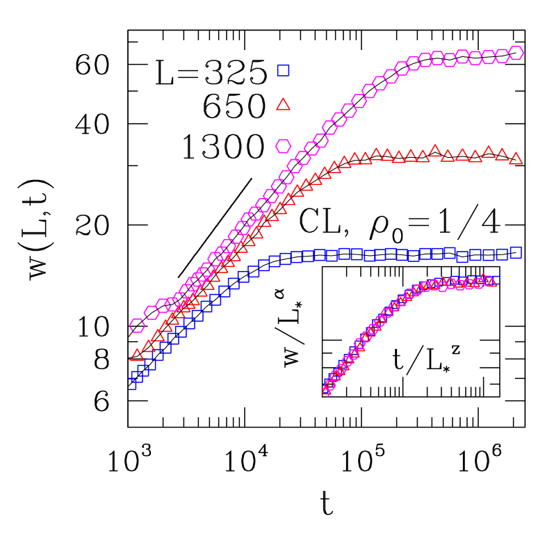
Figure 10: (Color online) Double-logarithmic plot of interface width against time, corresponding to TASEP with open boundary conditions on the coexistence line, at $\alpha_{I}=\beta_{E}=1/4$. Initial density $\rho_{0}=1/4$, lattice sizes $L$ as in key to symbols. Full line corresponds to $w\sim t^{0.47}$. Inset: scaling plot of data on main diagram, using $\alpha=1$, $z=2.1$; $L_{\ast}=L/325$.

Attempting curve collapse on the data of Fig. 10 (see inset) gives the following estimates: $\alpha=0.99(1)$, $z=2.10(5)$. This would imply $\beta=0.47(2)$ from scaling, as shown by the straight line on the main plot; a direct fit of $L=1300$ data for $7\times 10^{3}<t<7\times 10^{4}$ gives $\beta=0.39(1)$, which again is a larger discrepancy compared with the scaling prediction than in cases previously examined here.

The estimate of $z$ from curve collapse is roughly in line with the Bethe ansatz prediction ess05 $z=2$, though it seems difficult to stretch the error bars for our data to include this latter value. As regards $\alpha$, our estimate suggests that $\alpha=1$ is possibly an exact result for this case.

An argument can be given as follows. Going back to the calculation outlined, for PBC, in Eq. (7), and recalling the spatial phase segregation shown in the late-time data of Fig. 8, one sees that the dominant feature of the interface (particle system) is its division at a strongly fluctuating interface into two main segments with symmetric slopes (low and high densities), of lengths $\propto L$. In order words, local densities will be correlated along distances of order $L$. This is enough to guarantee that the mean square interface width will depend on $L^{2}$. This argument is supported by a calculation of the size dependence of the stationary mean square width. On the coexistence line the diffusing shock gives a linear average stationary density profile (refer to the late-time curves in Fig. 9), and this makes the large time limit of Eq. (7) proportional to $L^{2}\,(2\alpha_{I}-1)^{2}$ , consistent with $\alpha=1$.

III.2 Continuum mean-field approach

We investigate how the effects of number conservation can influence the approach to stationarity. We wish to find out whether, and under what conditions, transient (e.g., ballistic) phenomena can occur which would mask the underlying long-time relaxational dynamics. Determination of the exponent $z$ via interface width scaling, as done in Secs. II and III.1, relies heavily upon collapsing the ’shoulders’ which mark the final approach to stationarity, thus this method always picks out the longest characteristic time. Therefore one may ask, for the low-density phase with open boundary conditions, whether the $L-$independent relaxation time implied by the prediction $z=0$ is hidden underneath a longer process; and whether in this scenario the latter time, which is captured by interface width scaling, is associated with features not so far emphasised within Bethe ansatz investigations, as in the connection between ballistic motion and imaginary parts of energies. Such things might explain the seeming mismatch between our results and those of Ref. ess05, .

In the TASEP (and similar non-equilibrium flow processes) the bulk hopping process conserves total particle number - hence the continuity-equation nature of the evolution equation, and the slow nature of long-wavelength fluctuations of the density. With open boundaries, particles can appear and leave at the chain ends, thus causing the total number of particles inside to change.

A group of particles crossing at a boundary immediately affects the mean density and the local density near the boundary. Such a group may be transferred into the interior as a kinematic wave/moving domain wall provided the kinematic wave velocity $v$ is non-zero and of the right sign. A time of order $L/v$ will be needed to affect the local density throughout a system of size $L$ (as for example is typically required to achieve a steady state configuration).

This argument suggests that measurements of quantities (like ones conserved in the interior) whose changes are boundary-induced will show characteristic times of order $L^{\,z^{\prime}}$, with $z^{\prime}$ at least unity (still slower limiting processes may also be involved, owing to intrinsic features of the dynamics).

In order to provide a quantitative counterpart to these ideas, we have used a continuum mean-field approach (see, e.g., Ref. rbs01, ) in which the system is described by the noiseless Burgers/KPZ equations, linearized by the Cole-Hopf transformation hopf50 ; cole51 . This picks up the kinematic wave effects in the evolution of the local density $\rho_{\ell}$ and its mean $\rho$. It captures the ballistic transport between boundary and interior, described qualitatively above, which gives $z^{\prime}=1$. In this description the reduced density $\sigma_{\ell}(t)=\rho_{\ell}(t)-1/2$ evolves like:

$$\sigma_{\ell}(t)=\frac{\partial}{\partial\ell}\,\ln\{\cosh K(\ell-\ell_{0})\,e^{-K^{2}t}+$$

$$+{\sum_{k}}^{\prime}(A_{k}\,e^{k\ell}+B_{k}\,e^{-k\ell})\,e^{-k^{2}t}\}\ ,$$ (10)

towards a steady state:

$$\sigma_{\ell}=K\,\tanh K(\ell-\ell_{0})\ ,$$ (11)

where $K$ and $\ell_{0}$ are decided by boundary rates ($\alpha_{I},\beta_{E}$), $K$ being real, except in the MC phase where it is imaginary. The sum ${\sum}^{\prime}$ takes care of the difference between initial and steady states, and (since this difference is decaying) it involves complex $k$ with ${\rm Re}\,(k^{2})>K^{2}$; this $k$ has to be consistent with boundary conditions. $A_{k}$, $B_{k}$ are therefore determined by initial conditions. The difference typically becomes a kinematic wave or domain wall sch00 ; be07 ; lw55 ; djls03 ; ksks98 ; ps99 ; hkps01 ; sa02 . If it is kink–like, its velocity $v$ depends as follows on coarse-grained densities $\rho_{<}$, $\rho_{>}$ and currents $J_{<}$, $J_{>}$ on either side of the kink: $v=(J_{<}-J_{>})/(\rho_{<}-\rho_{>})$. These quantities are set by the steady-state and initial (uniform) density profiles; for smooth small–amplitude kinematic waves $v=dJ/d\rho=1-2\rho$, and then the local coarse-grained density $\rho$ is at late times set by the steady state.

For our investigations at $(\alpha_{I},\beta_{E})=(1/4,1/2)$ the initial profile $\rho_{\ell}=1/4$ has to go into the steady-state profile, which corresponds to $K=1/4$, $\ell_{0}=L$, and differs from the initial one only in having an upturn (to $\rho_{L}=3/8$) at the right boundary.

The kinematic wave velocity for $\rho=1/4$ is $1/2$, i.e., positive, so there is ballistic transfer, actually of vacancies at speed $1/2$ from the right boundary, which after time $t\simeq L/v=2L$ produces the steady-state profile with its upturn at the right boundary. This is corroborated by our numerical results depicted in Fig. 6. For all cases $L=325$, $650$, and $1300$, the interface width at $t=2L$ has reached more than $98\%$ of its asymptotic value. Thus, while attempts at producing overall curve collapse indicate $z^{\prime}\simeq 1.20$ as quoted above, by focusing exclusively on the scaling of the ’shoulders’ one gets a result much closer to the mean-field value.

We also applied this picture to other cases investigated in Subsection III.1, to check for consistency. Results are as follows.

For the MC phase at $(\alpha_{I},\beta_{E})=(3/4,3/4)$, initially $\rho_{\ell}=1/2$, so $v=0$ and the steady state $\rho_{\ell}$ differs from the average by an upturn to $2/3$ at the left boundary, and a downturn to $1/3$ at the right one. So ballistic effects are not very important; furthermore the limiting process is the slower "KPZ diffusion" having $z=3/2$.

On the coexistence line at $(\alpha_{I},\beta_{E})=(1/4,1/4)$, two initial densities were used: (a) $\rho_{\ell}=1/2$, (b) $\rho_{\ell}=1/4$. For (a), the essential aspects are all as given in Fig. 9, i.e., a ballistic early evolution from the domain walls coming in from either end, followed by the limiting slower diffusive process ($z=2$). These together give rise to the non-monotonic form in Fig. 7. For (b), the ballistic process is effective for a long time (of order $L$) during which the average $\rho$ builds up, but again the limiting process is diffusion ($z=2$).

So, the mean-field continuum picture is consistent with all our numerical results for open boundary conditions, especially the one where we differ from Ref. ess05, . In this latter case, the characteristic time arising from propagation of the kinematic wave is longer than the intrinsic ($L-$independent) one, thus resulting in the effective exponent $z^{\prime}=1$ (for all other cases, an exponent $z>1$ associated to intrinsic dynamics dominates anyway). Note that, for this scenario to work, one needs the kinematic wave to have non-zero effective velocity $v$, and (for a characteristic relaxation time, proportional to $L$, to show up) one also needs the kinematic wave to have to traverse a length of order $L$ – whether that is the case depends on the maximum distance from the nearest effective boundary to the place(s) where the profile has to be adjusted.

In summary, the difference between our results and those of Ref. ess05, is real, and interpretable as above. The effects and interpretation may be important for other quantities conserved in the bulk which build up only by propagation from the boundaries.

IV quenched disorder

Quenched disorder in the TASEP has been studied by many authors tb98 ; bbzm99 ; k00 ; ssl04 ; ed04 ; hs04 . Here, we investigate bond disorder k00 , i.e., while all particles are identical, the site-to-site hopping rates are randomly distributed.

Hereafter, we restrict ourselves to binary distributions $P(p)$ for the internal nearest-neighbor hopping rate $p$:

$$P(p)=\varphi\,\delta(p-p_{s})+(1-\varphi)\,\delta(p-p_{w})\ ,$$ (12)

where $p_{s}>1/2$, $p_{w}<1/2$ are associated, respectively, to "strong" and "weak" bonds.

One must recall that the bond disorder introduced above gives rise to correlated, or "columnar" disorder in the associated interface problem k00 ; ahhk94 . Indeed, the (fixed) value of the hopping rate at a given position $x$ along the particle-model axis will determine, once and for all, the probability of the height $h(x)$ being updated. This is in contrast with the usual picture of quenched disorder in the KPZ model l93 ; csahok93 ; opz95 ; amaral95 ; sak02 ; katsu04 , where it is assumed that the intensity of disorder is a random function of the instantaneous two-dimensional position $\left(x,h(x)\right)$ of the interface element at $x$.

In Figure 11 we show interface width data for PBC, $\rho=1/2$, and $\varphi=1/2$, $p_{s}=0.8$, $p_{w}=0.2$ in Eq. (12). Note that the relaxation times are one order of magnitude longer than is usual for pure systems (in the latter case, one must make exception for the coexistence line with open boundary conditions). Though the overall picture of a scaling regime still holds, with interface widths evolving in a simple, monotonic way, in general the quality of data collapse is lower than for pure systems. From our best fit, we estimate $\alpha=1.05(5)$, $z=1.7(1)$, from which scaling gives $\beta=0.62(7)$. A direct fit of $2\times 10^{3}\leq x\leq 2\times 10^{4}$ data for $L=1300$ gives $\beta=0.56(1)$, only just within the error bars predicted by scaling.

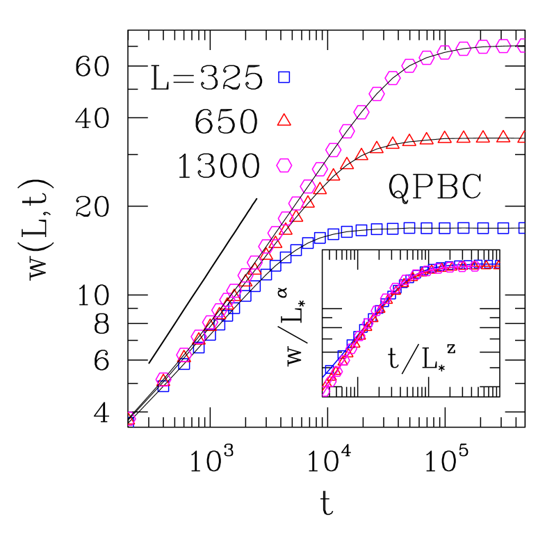
Figure 11: (Color online) Double-logarithmic plot of interface width against time, corresponding to TASEP with periodic boundary conditions and binary quenched disorder, with $\varphi=1/2$, $p_{s}=0.8$, $p_{w}=0.2$ [see Eq. (12)]. $\rho=1/2$, lattice sizes $L$ as in key to symbols. Full line corresponds to $w\sim t^{0.61}$. Inset: scaling plot of data on main diagram, using $\alpha=1.05$, $z=1.7$ (see text); $L_{\ast}=L/325$. Each point is an average over $10\,000$ independent realizations of quenched randomness.

We have examined the stationary-state slope distributions for the interface problem. Numerical results are displayed in Fig. 12, together with their fit by a double-Gaussian form, $\Phi(x)=a\,G_{1}(x)+(1-a)\,G_{2}(x)$, where $G_{i}$ is a Gaussian centered at $x_{i}$ with variance $\sigma_{i}^{2}$. The best-fitting parameters give a roughly symmetric curve, with $a=0.53(2)$, $x_{1}=-0.26(1)$, $x_{2}=0.31(1)$, $\sigma_{1}=0.21$, $\sigma_{2}=0.18$. Such a double-peaked structure indicates phase separation, as seen earlier for pure systems on the coexistence line (though here this is quantitatively milder, as the peak-to-trough ratio is $\sim 1.3$, to be compared to $\sim 8$ in the previous case). Phase separation is known to be a feature of the quenched-disordered TASEP tb98 .

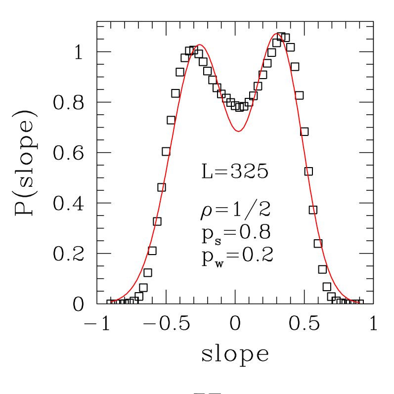
Figure 12: (Color online) Slope PDF in stationary state, corresponding to TASEP with quenched disorder, $\varphi=1/2$, $p_{s}=0.8$, $p_{w}=0.2$ [see Eq. (12)]. Lattice size $L=325$ with PBC, $\rho=1/2$. Full line is a double Gaussian fit to data (see text). $100$ independent realizations of quenched randomness were used, for each of which samples were collected from $3\times 10^{4}$ consecutive interface configurations.

We now outline a theoretical framework for the description of the quenched-disordered problem, in the spirit of earlier work by Tripathy and Barma tb98 . The analytic understanding of slope distributions and, particulary, of currents and profiles, rests on the division of the system, for a given disorder configuration, into an alternating succession of weak-bond and strong-bond segments (${\cal S}^{w}$ and ${\cal S}^{s}$) each containing only bonds of one strength. The longest weak bond segments determine the current through the system. This is easily seen in a mean field account of the steady state of the particle system (with PBC). Here the constant current $J$ yields the relation (profile map)

$$\rho_{\ell+1}=1-\frac{J}{p_{\ell}\,\rho_{\ell}}\ ,$$ (13)

where $p_{\ell}$ is the hopping rate from site $\ell$ to $\ell+1$, and $\rho_{\ell}$ is the mean occupation of site $\ell$.

Throughout a weak bond segment ${\cal S}^{w}_{n}$ of length $n$ the map involves the constant (reduced) current $J/p_{\ell}=J/p_{w}\equiv J_{w}$. The corresponding strong bond variable is $J/p_{s}\equiv J_{s}$; $J_{s}<J_{w}$ since $p_{s}>p_{w}$. So, within any ${\cal S}^{w}_{n}$ (or ${\cal S}^{s}_{n}$) the profile map is that of an effective pure system, which is well known to give density profiles of kink shape, corresponding to low current or high current: $\rho_{\ell}-\frac{1}{2}=k\,\tanh k(\ell-\ell_{0})$ (monotonic increasing) or $\rho_{\ell}-\frac{1}{2}=-K\tan K(\ell-\ell_{0})$ (monotonic decreasing), depending on whether the reduced current $J/p$ is less than or greater than $1/4$. $k$ and $K$ are related to the reduced current by $k=\sqrt{(1/4)-(J/p)}$; $K=\sqrt{(J/p)-(1/4)}$ hs04 .

In the high current case $K$ has to be small [$\,\lesssim{\cal O}(1/L)$ in a segment of size $L\,$], to prevent the tangent from diverging and taking $\rho_{\ell}$ outside of the permitted physical range $[0,1]$. In the binary random system, it is not possible to have both weak and strong bond segments (having respectively $K=K_{w}$, $K_{s}$) in the high current ’state’ since that would lead to monotonically decreasing $\rho$ for all segments. That would violate the periodic boundary condition requirement. It cannot even apply with open boundary conditions in a large system, because even with $K_{s}$ kept small by having $J_{s}$ close to $1/4$, the larger $J_{w}$ would cause a large $K_{w}$, resulting in non-physical values of $\rho_{\ell}$. Arguments of this sort show that the strong bond segments ${\cal S}^{s}$ are all in the low current phase, i.e., $J_{s}<1/4$ with density profiles in each ${\cal S}^{s}$ increasing monotonically. Thus, for PBC the profiles in each ${\cal S}^{w}$ have to decrease. That can come about from having $J_{w}>1/4$, which leads to $K_{w}=\sqrt{J_{w}-(1/4)}$. If the longest weak bond segment has length $n_{0}$, to prevent unphysical $\rho_{\ell}$’s resulting from a divergence of $\tan K_{w}(\ell-\ell_{0})$ somewhere within that segment we must have $K_{w}\leq\pi/n_{0}$. This gives:

$$\frac{1}{4}\leq\frac{J}{p_{w}}\lesssim\frac{1}{4}+\left(\frac{\pi}{n_{0}}\right)^{2}\ .$$ (14)

It is straightforward to show that the characteristic length of weak bond segment is $n\sim\ln\left(1/(1-\varphi)\right)$, and the largest weak segment length is $n_{0}\sim\ln L/\ln\left(1/(1-\varphi)\right)$, so the above condition on $J_{w}$ is very restrictive, making the current typically $J\sim(p_{w}/4)+{\cal O}\left((1/\ln L)^{2}\right)$.

This is in agreement with simulation results $J\simeq 0.055$ and $0.029$, respectively for $p_{w}=0.2$ and $p_{w}=0.1$ (both with $\rho=1/2$ on a lattice with $L=325$).

A decreasing profile in each ${\cal S}^{w}$ is also possible with $J_{w}$ slightly less than $1/4$ since, in addition to the kink-shaped low current profile, a profile with $\rho_{\ell}$ decreasing between $1$ and $(1/2)+k$ can result from the low current map. Again the $K_{w}$ that allows that is limited, leading for this case to $J\sim(p_{w}/4)-{\cal O}\left((1/\ln L)^{2}\right)$. This was seen, for example, in simulations for $\rho=0.8$, where $p_{w}=0.1$ gives $J\simeq 0.024$. This same result can also arise from another low current profile (having $\rho_{\ell}$ decreasing between $(1/2)-k$ and zero). All these weak segment profiles are seen in simulation results, together with the characteristic kink-shaped profiles of the strong-bond segments (e.g., for $p_{w}=0.1$, $\rho=0.5$ see Fig. 13, having $J=0.0297(3)$, i.e., $J/p_{w}$ just greater than $1/4$).

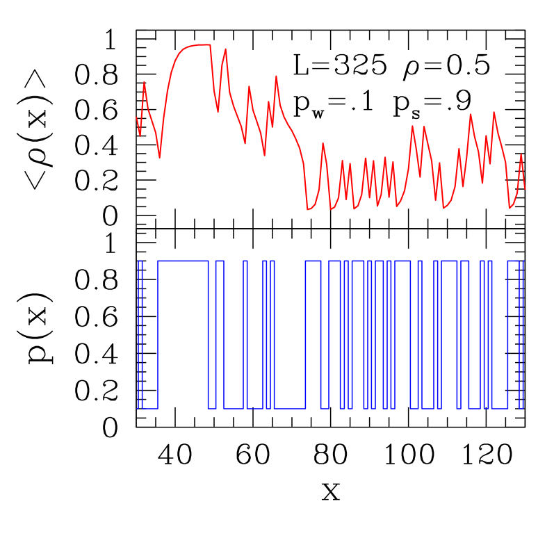
Figure 13: (Color online) Upper part: time-averaged particle density against position on section of $L=325$ system with PBC, corresponding to TASEP with quenched disorder, for a fixed bond configuration (seen in lower part of figure). Overall density $\rho=1/2$, $\varphi=1/2$, $p_{s}=0.9$, $p_{w}=0.1$ [see Eq. (12)]. Average is over $4.65\times 10^{5}$ successive time steps, in stationary state. Note kink-shaped profile for $35\lesssim x\lesssim 45$, in direct correspondence with the longest concentration of strong bonds; also, the high-current profile for $65\lesssim x\lesssim 75$, coinciding with the longest concentration of weak bonds.

Local density or slope distributions $P(\sigma)$, with $\sigma\equiv\partial h/\partial x$, are available from the profiles $\rho_{\ell}$, just as for the pure case, by using the known density-slope relation, Eq. (2) in:

$$P(\sigma)=\sum_{\rm segments}\int d\sigma_{\ell}\,\frac{\delta(\sigma-\sigma_{\ell})}{|\,d\sigma_{\ell}/d\ell\,|}=\sum_{\rm segments}\frac{1}{|\,d\sigma_{\ell}/d\ell\,|}_{\sigma_{\ell}=\sigma}\ .$$ (15)

Contributions from high current segments give (using $\sigma_{\ell}=-K\tan K\ell\,$):

$$C\equiv\frac{1}{|\,d\sigma_{\ell}/d\ell\,|}_{\sigma_{\ell}=\sigma}=2\left[\sigma^{2}+4K^{2}\right]^{-1}\ ,$$ (16)

while low current segments have contributions

$$C=\begin{cases}{2\left[4k^{2}-\sigma^{2}\right]^{-1}\quad{\rm for}\ |\,\sigma|<2k}\cr{2\left[\,\sigma^{2}-4k^{2}\right]^{-1}\quad{\rm for}\ |\,\sigma|>2k\ .}\end{cases}$$ (17)

In Eqs. (16), (17), these contributions are superimposed with $\varphi$–dependent weights related to their frequency of occurrence. Stochastic effects, missed from this account, cause fluctuations in the spatial pinning of the profiles (as for the pure case), leading mainly to a smoothing of the divergences near $\sigma=\pm 2k$ in the low current segment contributions. Quantitative comparison of these predictions, e.g., to the data displayed in Fig. 12, is not entirely appropriate, on account of the coarse-graining introduced by taking slope samples along segments of size $m$ bonds (typically $m=60$, as mentioned above). Nevertheless, one can see that some general aspects, such as the appearance of peaks roughly equidistant from $\sigma=0$, are effectively mirrored in the numerical results.

V Discussion and Conclusions

We start our discussion by recalling that the thermodynamic limits of interface models, such as KPZ, and of exclusion processes, differ in a subtle way. Namely, as can be seen from Eqs. (5) and (6), if one takes the $L\to\infty$ limit before allowing $t\to\infty$, one is left with a perpetual coarsening transient in which the interface gets ever rougher. On the other hand, the TASEP displays a well-defined stationary state even on an infinite system. Therefore, the correspondence of the limiting-width regime of the former type of problem to the stationary state of the latter can be only take effect within a finite-size scaling context.

Once one is mindful of this distinction, however, the similarities and differences between two finite systems linked by the correspondence recalled in Sec. I are expected to be bona fide features, which reflect objective connections between the physics of non-equilibrium flow processes, and that of moving interfaces in random media.

In Sec. II we first confirmed that the known KPZ exponents can be numerically extracted, with good accuracy, from the scaling of interface widths derived from the underlying TASEP with PBC. For a given range of system sizes, direct evaluation of $\beta$ by examination of the transient regime of width growth against time seems to be the least accurate procedure, which in this case gave $\beta=0.31(1)$. From scaling, with $\alpha=0.500(5)$, $z=1.52(3)$, one gets $\beta=0.33(1)$, in much better agreement with the exact $\beta=1/3$. Measuring this exponent directly from the transient regime tends to result in underestimation; as seen in Secs. III and IV above, such a trend is present in all our subsequent results, both for open systems and for quenched disorder. Also for PBC, we showed that the dependence of limiting KPZ interface widths against TASEP particle density can be accounted for by a treatment, which makes explicit use of the weight factorization that occurs for TASEP with PBC derr93 ; derr98 . Arguments based on weight factorization provide an explanation for the shape of slope distributions in the interface problem as well.

In Subsec. III.1, we first established that open-boundary systems in the maximal-current phase, characterized by $\alpha_{I}$, $\beta_{E}\geq 1/2$, exhibit the same set of KPZ exponents as their PBC counterparts. For the exponent $z$, this is in agreement with the Bethe ansatz solution ess05 . Examination of interface widths corresponding to systems in the low-density phase, with $\alpha_{I}=1/4$, $\beta_{E}=1/2$, shows that curve collapse can be found to a rather good extent, giving the following exponent estimates: $\alpha=0.497(3)$, $z=1.20(5)$, $\beta=0.41(2)$. This apparent disagreement with the Bethe ansatz prediction ess05 of $z=0$, which implies a finite correlation length, is addressed in Subsec. III.2 (see two paragraphs on). We have been able to provide a prediction of the (possibly exact) interface width exponent $\alpha=1/2$, based on considerations which make explicit use of a finite correlation length for the TASEP.

For systems with $\alpha_{I}=\beta_{E}<1/2$, i.e., on the coexistence line of the open-boundary TASEP, interface width scaling gave $\alpha=0.99(1)$, $z=2.10(5)$, $\beta=0.47(2)$. We provided a prediction of $\alpha=1$ based on properties of the corresponding TASEP, in this case the fact that phase separation governs the dominant features of the interface configuration at stationarity. Direct calculation of density profiles in the particle system shows the time evolution of a shock (kinematic wave). At late times, the ensemble-averaging of local densities tends to mask the evidence of phase segregation, which can, however, be retrieved by examination of the corresponding interface slope PDFs.

In Subsec. III.2, we outlined a mean-field continuum calculation, which sheds additional light on the approach to stationarity in open-boundary systems. We showed that, under suitable conditions such as those at $(\alpha_{I},\beta_{E})=(1/4,1/2)$ with uniform initial density $\rho_{\ell}=1/4$, system-wide propagation of a kinematic wave translates into a characteristic time $\propto L^{\,z^{\prime}}$ ($z^{\prime}=1$ in mean field). This goes towards explaining the apparent inconsistency between our result from interface-width evolution, $z=1.20(5)$, and that from the Bethe ansatz solution which gives $z=0$. Indeed, in that case the $L-$independent relaxation time implied by $z=0$ is hidden underneath a slower part of ballistic origin, and it is the scaling of the latter which is captured by the interface width collapse, but not by considerations solely of the real part of Bethe ansatz excitation energies. Furthermore, in all other cases where our own numerical results are consistent with those of Ref. ess05, , the mean-field prediction concurs with both. An extension of this work has now been carried out using the more precise domain wall method of Refs. ksks98, ; ds00, on a kink–like initial state in the massive phase fab-p . This shows clearly the ballistic element and the much faster (size-independent) amplitude decay, providing an independent confirmation of the scenario.

In Sec. IV we investigated quenched bond disorder in TASEP with PBC. From the scaling analysis of the corresponding interface widths (which in this case are subjected to correlated, or "columnar" randomness k00 ; ahhk94 ) we estimate $\alpha=1.05(5)$, $z=1.7(1)$, $\beta=0.62(7)$. For comparison, values quoted for $\beta$ in standard, two-dimensional quenched disorder in $D=1+1$ KPZ systems are close to $0.63$ csahok93 ; opz95 . It has been argued opz95 ; amaral95 that this type of KPZ model is in the universality class of directed percolation, thus one should have $\beta=\beta_{DP}=0.633$. Furthermore, in Ref. amaral95, , it is shown that by varying the intensity of the various terms in the quenched counterpart of Eq. (3), one can make KPZ-like systems go through distinct regimes, namely: pinned, with $\alpha_{P}=0.63(3)$, $\beta_{P}=0.67(5)$, $z_{P}=1.06(8)$; moving, with $\alpha_{M}=0.75(4)$, $\beta_{M}=0.74(6)$, $z_{M}=1.01(10)$; and annealed (i.e., fast-moving interface), with $\alpha_{A}=0.50(4)$, $\beta_{A}=0.30(4)$, $z_{A}=1.67(26)$. It can be seen that our own set of estimates does not fully fit into any of these, as could reasonably be expected from the extreme correlation between quenched defects which is present here, and not in those early examples.

We tested universality properties within the columnar disorder class of models. This was done by replacing the binary distribution, Eq. (12), with a continuous, uniform one: $P(p)=(1-c)^{-1}$ for $c<p<1$. We used $c=0.1$, thereby avoiding the problems associated with allowing $p=0$, see Ref. k00, , while still having a rather broad distribution. Our data scale similarly to those displayed in Figure 11 for Eq. (12). We get $\alpha=1.05(5)$, $z=1.45(10)$ (hence $\beta=0.72(7)$ from scaling), in reasonable agreement with the binary disorder case, though error bars for $z$ just fail to overlap.

We also investigated slope distributions for the quenched disorder problem. These provide clear evidence of phase separation, a phenomenon known to take place in such circumstances tb98 .

A direct analytic (mean-field) approach to steady-state properties of TASEP with quenched disorder produced closed-form expressions for the piecewise shape of averaged profiles densities, as well as rather restrictive bounds on currents. All these have been verified in our numerical simulations. The analytic approach is similar to that of Ref. tb98, , where it was already shown that a mean field description applies, and to part of Ref. hs04, . In place of the maximum current principle used in Ref. tb98, we have obtained analytic consequences of the mean field mapping within segments and combined them with segment probabilities to obtain new results, particularly for profiles and limiting currents.

We note that, for weak randomness, characterized by a small value of a disorder parameter $\varepsilon$ [this could be, e.g., $p_{s}-p_{w}$ in Eq. (12)], and steady state conditions, the noiseless (mean-field) constant current condition gives an equation for $\sigma\equiv\partial h/\partial x$ in the form:

$$\varepsilon\,\zeta(x)=\frac{\partial\sigma}{\partial x}+\sigma^{2}\ ,$$ (18)

where $\zeta(x)$ is a quenched variable corresponding to random bond disorder. Eq. (18) has the same structure as that found for equations governing the evolution of local Lyapunov exponents for Heisenberg-Mattis spin glass chains dqrbs06 ; dqrbs07 . To see the correspondence, refer, e.g., to Equation (14) of Ref. dqrbs07, , substituting $\varepsilon$ for (low) magnon frequency $\omega$. So one can, in principle, adopt the same type of Fokker-Planck procedures to find distributions of $\sigma$ in Burgers-like equations, and hence of slope distributions in KPZ systems.

- (1) B. Derrida, Phys. Rep. 301, 65 (1998).
- (2) M. Kardar, G. Parisi, and Y.-C. Zhang, Phys. Rev. Lett. 56, 889 (1986).
- (3) T. Halpin-Healy and Y.-C. Zhang, Phys. Rep. 254, 215 (1995).
- (4) A.-L. Barábasi and H. E. Stanley, Fractal Concepts in Surface Growth (Cambridge University Press, Cambridge, 1995).
- (5) G. M. Schütz, in Phase Transitions and Critical Phenomena, edited by C. Domb and J. L. Lebowitz (Academic, New York, 2000), Vol. 19.
- (6) B. Derrida, M. Evans, V. Hakim, and V. Pasquier, J. Phys. A 26, 1493 (1993).
- (7) P. Meakin, P. Ramanlal, L. M. Sander, and R. C. Ball, Phys. Rev. A34, 5091 (1986).
- (8) J. Krug and H. Spohn, in Solids Far from Equilibrium, edited by C. Godreche (Cambridge University Press, Cambridge, England, 1991), and references therein.
- (9) T. Kriecherbauer and J. Krug, arXiv:0803.2796 (2008); see especially Sec. 4.
- (10) D. Forster, D. R. Nelson, and M. J. Stephen, Phys. Rev. A16, 732 (1977).
- (11) H. van Beijeren, R. Kutner, and H. Spohn, Phys. Rev. Lett. 54, 2026 (1985).
- (12) B. Derrida, E. Domany, and D. Mukamel, J. Stat. Phys. 69, 667 (1992).
- (13) D. Kandel, G. Gershinsky, D. Mukamel, and B. Derrida, Phys. Scr. T49, 622 (1993).
- (14) M. Depken and R. Stinchcombe, Phys. Rev. Lett. 93, 040602 (2004).
- (15) R. B. Stinchcombe, Adv. Phys. 50, 431 (2001).
- (16) R. A. Blythe and M. R. Evans, J. Phys. A 40, R333 (2007).
- (17) Z. Nagy, C. Appert, and L. Santen, J. Stat. Phys. 109, 623 (2002).
- (18) J. de Gier and F. H. L. Essler, Phys. Rev. Lett. 95, 240601 (2005); J. Stat. Mech.: Theory Exp. (2006) P12011.
- (19) E. Hopf, Commun. Pure Appl. Math. 3, 201 (1950).
- (20) J. D. Cole, Quart. Appl. Math. 9, 225 (1951).
- (21) M. J. Lighthill and G. B. Whitham, Proc. Roy. Soc. A 229, 317 (1955).
- (22) B. Derrida, S. A. Janowsky, J. L. Lebowitz, and E. R. Speer, J. Stat. Phys. 73, 813 (1993).
- (23) A. B. Kolomeisky, G. M. Schütz, E. B. Kolomeisky, and J. P. Straley, J. Phys. A 31, 6911 (1998).
- (24) V. Popkov and G. Schütz, Europhys. Lett. 48, 257 (1999).
- (25) J. S. Hager, J. Krug, V. Popkov, and G. M. Schütz, Phys. Rev. E63, 056110 (2001).
- (26) L. Santen and C. Appert, J. Stat. Phys. 106, 187 (2002).
- (27) G. Tripathy and M. Barma, Phys. Rev. E58, 1911 (1998).
- (28) M. Bengrine, A. Benyoussef, H. Ez-Zahraouy, and F. Mhirech, Phys. Lett. A 253, 135 (1999).
- (29) J. Krug, Braz. J. Phys. 30, 97 (2000).
- (30) L. B. Shaw, J. P. Sethna, and K. H. Lee, Phys. Rev. E70, 021901 (2004).
- (31) C. Enaud and B. Derrida, Europhys. Lett. 66, 83 (2004).
- (32) R. J. Harris and R. B. Stinchcombe, Phys. Rev. E70, 016108 (2004).
- (33) I. Arsenin, T. Halpin-Healy, and J. Krug, Phys. Rev. E49, R3561 (1994) .
- (34) H. Leschhorn, Physica A 195, 324 (1993).
- (35) Z. Csahók, K. Honda, E. Somfai, M. Vicsek, and T. Vicsek, Physica A 200, 136 (1993).
- (36) Z. Olami, I. Procaccia, and R. Zeitak, Phys. Rev. E52, 3402 (1995).
- (37) Luis A. Nunes Amaral, A.-L. Barábasi, H. A. Makse, and H. E. Stanley, Phys. Rev. E52, 4087 (1995).
- (38) G. Szabó, M. Alava, and J. Kertész, Europhys. Lett. 57, 665 (2002).
- (39) H. Katsuragi and H. Honjo, J. Phys. Soc. Jpn. 73, 3087 (2004).
- (40) M. Dudzinski and G. M. Schütz, J. Phys. A 33, 8351 (2000).
- (41) F. Essler, private communication.
- (42) S. L. A. de Queiroz and R. B. Stinchcombe, Phys. Rev. B73, 214421 (2006).
- (43) S. L. A. de Queiroz and R. B. Stinchcombe, Phys. Rev. B76, 184421 (2007).