Heterogeneous credit portfolios and the dynamics of the aggregate losses

Abstract

We study the impact of contagion in a network of firms facing credit risk. We describe an intensity based model where the homogeneity assumption is broken by introducing a random environment that makes it possible to take into account the idiosyncratic characteristics of the firms. We shall see that our model goes behind the identification of groups of firms that can be considered basically exchangeable. Despite this heterogeneity assumption our model has the advantage of being totally tractable. The aim is to quantify the losses that a bank may suffer in a large credit portfolio. Relying on a large deviation principle on the trajectory space of the process, we state a suitable law of large number and a central limit theorem useful to study large portfolio losses. Simulation results are provided as well as applications to portfolio loss distribution analysis.

Keywords: Central limit theorems in Banach spaces, Credit contagion, intensity based models, Large Deviations, large portfolio losses, random environment.

AMS 2000 subject classifications: 60K35, 91B70

Introduction

During the last years the challenging issue of describing the dynamics of the loss process connected with portfolios of many obligors has received more and more attention. Applications can be found both for management purposes (see [8]) and in the literature dealing with pricing and hedging of risky derivatives as CDOs (Collateralized Debt Obligations). For a discussion of this framework see [15] and [18].

When dealing with portfolio losses, it becomes crucial the modeling of the dependence structure among the obligors. One standard procedure is to directly specify the intensity of default of the single obligors belonging to the portfolio in order to infer the dynamics of the global system and thus the distribution of the aggregate losses. In the context of reduced form models a rather general framework is the conditionally Markov modeling approach by Frey and Backhaus (see [12] and [13]). One drawback of the intensity based models is the difficulty in managing large heterogeneous portfolios because of the presence of many obligors with different specifications. In this case it is common practice to assume homogeneity assumptions in order to reduce the complexity of the problem. A typical approach is to divide the portfolio into groups where the obligors may be considered exchangeable.

In this paper we describe an intensity based model where the homogeneity assumption is broken by introducing a random environment that makes it possible to take into account the idiosyncratic characteristics of the firms. We shall see that our model goes behind the identification of groups of firms that can be considered basically exchangeable. Despite this heterogeneity assumption our model has the advantage of being totally tractable.

The goal is to describe the evolution of the losses for a large portfolio where heterogeneity and direct contagion among the firms are taken into account. We denote by $L^{N}(t)$ the random variable describing the losses at time $t\in[0,T]$ for a portfolio of size $N$. Our approach works as follows. First we study the $N\to\infty$ limiting distributions on the path space of some aggregate variables useful to characterize the evolution of $L^{N}(t)$ for $t\in[0,T]$. To this effect we shall derive an appropriate Law of Large Numbers based on a Large Deviations Principle in order to describe a limiting behavior that can be considered as a asymptotic regime with infinite firms. Finally, we study the finite volume approximations (for finite but large $N$) of the limiting distribution via a suitable version of the Central Limit Theorem that describes the fluctuations around this limit. In most cases, these dynamical fluctuation theorems are proved by method of weak convergence of processes; this approach has been widely applied to models close in spirit to this work. We quote [12] and [7] for applications to finance. The effectiveness of those methods for heterogeneous models is, however, unclear. We follow here a different approach, which allows to prove a Central Limit Theorem directly in the underlying trajectory space. This approach is based on a general Central Limit Theorem in [3]. Although various applications of this theorem to fluctuations of Markov processes can be found in the literature (see e.g. [1] and [6]), to our knowledge the first application to a non-reversible Markov process.

In the risk management context, our model may be useful for the management of large portfolios, in the spirit of other models proposed in [16] or in [7]. It has been remarked that in many real world applications default are rather rare events, so that, for instance, the fraction of defaulted firms is close to zero and a normal approximations is not meaningful. Our models and results are only concerned with time scales for which a proper fraction of the portfolio is likely to be affected by the defaults.

We believe that our paper may be considered as an original contribution in the modeling of portfolio losses dynamics that accounts for both heterogeneity and contagion. On the other hand, to our knowledge, this is the first attempt to apply large deviations and normal fluctuation theory on path spaces (that is, in a dynamic fashion) for finance or credit management purposes, except for what contained in[7]. For a survey on large deviations methods applied to finance and credit risk see [17].

The models we propose in this paper are the simplest heterogeneous models describing systems comprised by many defaultable components, whose defaults are positively correlated via an interaction of mean-field type, i.e. with no geometric structure. Although we have been inspired by financial applications, we believe the basic principles should apply to other contexts.

The outline of this paper is as follows. In Section 1 we illustrate the model and the main theorems. In Section 2 we apply these results to the large portfolio losses analysis. Some examples with explicit computations and simulations are also provided. In Section 3 we conclude. Appendix A is devoted to the proofs of the three main theorems stated in Section 1.

1 Model and main results

Consider a network of $N$ defaultable firms, whose states are denoted by $y_{1},y_{2},\ldots,y_{N}$, $y_{i}\in\{0,1\}$. The event $\{y_{i}=1\}$ means that the $i$-th firm has defaulted. The values $y_{1},y_{2},\ldots,y_{N}$ give rise to an aggregate variable $m_{N}$ which indicates the global state of the network:

$$m_{N}:=\frac{1}{N}\sum_{i=1}^{N}\alpha_{i}y_{i},$$

where $\alpha_{1},\alpha_{2},\ldots,\alpha_{N}$ are given nonnegative numbers. $\alpha_{i}$ can be interpreted as the impact the default of the $i$-th firm has on the aggregate variable $m_{N}$. In order to model contagion, we assume the instantaneous rate of default of the $i$-th firm is an increasing function of $m_{N}$. More specifically, we assume the rate of default of the $i$-th firm is given by

$$I\!\!\!I\,_{\{y_{i}=0\}}e^{\beta_{i}m_{N}-\gamma_{i}},$$

where $I\!\!\!I\,_{A}$ is the indicator function of the set $A$, and $\beta_{i}\geq 0$, $\gamma_{i}\in{\mathbb{R}}$ are given constant. $\beta_{i}$ represents the sensibility of the $i$-th firm to variations of the aggregate variable $m_{N}$, while $\gamma_{i}$ can be interpreted as the “robustness” of the $i$-th firm: a large value of $\gamma_{i}$ means that the $i$-th firm is very unlikely to default within a given time.

Thus, for any fixed value of $\underline{\alpha}:=(\alpha_{1},\alpha_{2},\ldots,\alpha_{N})$, $\underline{\beta}:=(\beta_{1},\beta_{2},\ldots,\beta_{N})$ and $\underline{\gamma}:=(\gamma_{1},\gamma_{2},\ldots,\gamma_{N})$, the variable $\underline{y}:=(y_{1},y_{2},\ldots,y_{N})$ evolves as a Markov chain in continuous time, with infinitesimal generator given by

$${\cal{L}}_{\underline{\alpha},\underline{\beta},\underline{\gamma}}f(\underline{y}):=\sum_{i=1}^{N}I\!\!\!I\,_{\{y_{i}=0\}}e^{\beta_{i}m_{N}-\gamma_{i}}[f(\underline{y}^{i})-f(\underline{y})],$$ (1.1)

where $\underline{y}^{i}$ denotes the configuration obtained from $\underline{y}$ by changing $y_{i}$ from $0$ to $1$. We assume the system start at time $t=0$ from the configuration $\underline{y}(0)=(0,0,\ldots,0)$. The evolution randomly drives the network towards the trap state $(1,1\ldots,1)$, which is reached in finite time.

From now on we denote by $\lambda_{i}:=(\alpha_{i},\beta_{i},\gamma_{i})$ the triple of the parameters corresponding to the $i$-th firm. The $\lambda_{i}$’s model the heterogeneity of the system. We consider here the point of view of disordered models, i.e. we assume $\lambda_{1},\lambda_{2},\ldots,\lambda_{N}$ to be i.i.d. random variables, with a given law $\mu$. In order to avoid inessential difficulties, the law $\mu$ is assumed to have compact support in ${\mathbb{R}}^{+}\times{\mathbb{R}}^{+}\times{\mathbb{R}}$. Note that, for a given $i$, the random variables $\alpha_{i},\beta_{i},\gamma_{i}$ are not assumed to be independent. Sometimes, the vector $\underline{\lambda}:=(\lambda_{1},\lambda_{2},\ldots,\lambda_{N})$ will be referred to as random environment.

Consider a time $T>0$, and denote by $\underline{y}[0,T]=(\underline{y}(t))_{t\in[0,T]}$ the trajectory described by the configuration under the stochastic evolution (1.1). Each component $y_{i}[0,T]$ is either identically $0$ or it flips from $0$ to $1$ at the default time

$$\tau_{i}:=\inf\{t>0:y_{i}(t)=1\}.$$ (1.2)

By convention, we set $y_{i}(\tau_{i})=1$. This set of $\{0,1\}$-valued trajectories is denoted by ${\cal{D}}[0,T]$. Each trajectory in ${\cal{D}}[0,T]$ can be identified with its default time (which is set to be equal to $T$ if there is no default); thus ${\cal{D}}[0,T]$ inherits the topology induced by the usual topology on ${\mathbb{R}}$ for the default time. Equivalently, the topology on ${\cal{D}}[0,T]$ is the one induced by the Skorohod topology on the set of ${\mathbb{R}}$-valued functions which are right-continuous and admit limit from the left at any point of $[0,T]$ (see e.g. [11]).

In this paper we are interested in the asymptotic behavior, as $N\rightarrow+\infty$, of empirical averages of the form

$$\frac{1}{N}\sum_{i=1}^{N}f(y_{i}[0,T])=:\int fd\rho_{N}(\underline{y}[0,T]),$$

where $f:{\cal{D}}[0,T]\rightarrow{\mathbb{R}}$ is a Borel measurable function, and

$$\rho_{N}(\underline{y}[0,T]):=\frac{1}{N}\sum_{i=1}^{N}\delta_{y_{i}[0,T]}$$

is called empirical measure. More generally, we shall consider the empirical measure

$$\rho_{N}(\underline{y}[0,T],\underline{\lambda}):=\frac{1}{N}\sum_{i=1}^{N}\delta_{y_{i}[0,T],\lambda_{i}},$$

which is a random measure on ${\cal{D}}[0,T]\times{\mathbb{R}}^{3}$. Note that $\rho_{N}(\underline{y}[0,T])$ is the marginal of $\rho_{N}(\underline{y}[0,T],\underline{\lambda})$ on ${\cal{D}}[0,T]$.

In what follows, we denote by ${\cal{M}}_{1}$ the set of probability measures on ${\cal{D}}[0,T]\times Supp(\mu)$, while ${\cal{M}}$ will denote the set of signed measure on ${\cal{D}}[0,T]\times{\mathbb{R}}^{3}$. Both sets are provided with the weak topology.

For $y[0,T]\in{\cal{D}}[0,T]$ with $y(T)=1$, we set

$$\tau(y[0,T]):=\inf\{t>0:y(t)=1\}.$$

For $Q\in{\cal{M}}$ we define

$$F(Q):=\int Q(dy[0.T],d\lambda)\left\{\int_{0}^{T}(1-y(t))\left(1-e^{-\gamma}e^{\beta\int Q(d\eta[0,T],d\lambda^{\prime})\alpha^{\prime}\eta(t)}\right)dt\right.\\ +\left.y(T)\left[-\gamma+\left(\beta\int Q(d\eta[0,T],d\lambda^{\prime})\alpha^{\prime}\eta(t^{-})\right)\Big{|}_{t=\tau(y[0,T])}\right]\right\},$$ (1.2)

where $\lambda=(\alpha,\beta,\gamma)$ and $\lambda^{\prime}=(\alpha^{\prime},\beta^{\prime},\gamma^{\prime})$. For a fixed $\underline{\lambda}$, the infinitesimal generator (1.1), together with the initial condition $\underline{y}(0)=(0,0,\ldots,0)$ induces a probability $P_{N}^{\underline{\lambda}}$ on ${\cal{D}}^{N}[0,T]$. We think of $P_{N}^{\underline{\lambda}}$ as the conditional law of the process given the random environment. We denote by

$$P_{N}(d\underline{y}[0,T],d\underline{\lambda}):=P_{N}^{\underline{\lambda}}(d\underline{y}[0,T])\otimes\mu^{\otimes N}(d\underline{\lambda})$$

the joint law of the process and the environment. The distribution of $\rho_{N}(\underline{y}[0,T],\underline{\lambda})$ under $P_{N}$ will be denoted by $P_{N}\circ\rho_{N}^{-1}$.

A special case is when all components of $\underline{\lambda}$ are zero. In this case each firm defaults with rate $1$, independently of the others. We denote by $W$ the law on ${\cal{D}}[0,T]$ of this process.

In what follows, for $Q_{1},Q_{2}\in{\cal{M}}_{1}$, we denote by

$$H(Q_{1}|Q_{2}):=\left\{\begin{array}[]{ll}\int dQ_{2}\left(\frac{dQ_{1}}{dQ_{2}}\log\frac{dQ_{1}}{dQ_{2}}\right)&\mbox{if }Q_{1}\ll Q_{2}\mbox{ and }\frac{dQ_{1}}{dQ_{2}}\log\frac{dQ_{1}}{dQ_{2}}\in L^{1}(Q_{2})\\ +\infty&\mbox{otherwise}\end{array}\right.$$

the relative entropy of $Q_{1}$ with respect to $Q_{2}$.

Theorem 1

. The sequence $P_{N}\circ\rho_{N}^{-1}$ of elements of ${\cal{M}}_{1}$ satisfies a Large Deviation Principle (LDP) with good rate function

$$I(Q):=H(Q|W\otimes\mu)-F(Q).$$

The proof of Theorem 1, as well as of the other results stated in this section, is postponed to the appendix.
We recall that the above statement means that, for each Borel subset $A$ of ${\cal{M}}_{1}$,

$$-\inf_{Q\in{\buildrel{}_{\circ}\over{\mathrm{A}}}}I(Q)\leq\liminf_{N\rightarrow+\infty}\frac{1}{N}\log P_{N}\circ\rho_{N}^{-1}(A)\leq\limsup_{N\rightarrow+\infty}\frac{1}{N}\log P_{N}\circ\rho_{N}^{-1}(A)\leq-\inf_{Q\in\overline{A}}I(Q),$$

where ${\buildrel{}_{\circ}\over{\mathrm{A}}}$ and $\overline{A}$ denote the interior and the closure of $A$ respectively; moreover the function $I(\cdot)$ is nonnegative, lower-semicontinuous, and the level sets $\{Q:I(Q)\leq l\}$ are compact, for each $l>0$.

Theorem 2

. The equation $I(Q)=0$ has a unique solution $Q_{*}$, that can be identified as follows. Consider the nonlinear integro-differential equation

$$\left\{\begin{array}[]{rcl}\frac{\partial}{\partial t}q_{t}(\lambda)&=&e^{-\gamma}\exp\left[\beta\int\mu(d\lambda^{\prime})\alpha^{\prime}q_{t}(\lambda^{\prime})\right](1-q_{t}(\lambda))\\ q_{0}(\lambda)&\equiv&0\end{array}\right.$$ (1.3)

for a real-valued $q_{t}(\lambda)$, $t\geq 0$, $\lambda=(\alpha,\beta,\gamma)\in{\mathbb{R}}^{3}$. This equation has a unique solution $0\leq q_{t}(\lambda)\leq 1$. For every $\lambda$ fixed, consider the Markov chain on $\{0,1\}$ with time-dependent infinitesimal generator

$$L_{t}^{\lambda}f(s):=c_{t}^{\lambda}(s)[f(1-s)-f(s)],$$ (1.4)

where

$$c_{t}^{\lambda}(s):=(1-s)e^{-\gamma}\exp\left[\beta\int\mu(d\lambda^{\prime})\alpha^{\prime}q_{t}(\lambda^{\prime})\right]$$

and starting from $s=0$ (note that this process jumps only once, from $0$ to $1$, and it is then trapped in $1$). Let $Q_{*}^{\lambda}$ be the law of this process on ${\cal{D}}[0,T]$. Then

$$Q_{*}=Q_{*}^{\lambda}\otimes\mu.$$

Moreover

$$q_{t}(\lambda)=Q_{*}^{\lambda}(y(t)=1).$$

Theorems 1 and 2 have a simple consequence. Let $U$ be an open neighborhood of $Q^{*}$ in ${\cal{M}}_{1}$. By Theorem 2, lower semicontinuity of $I(\cdot)$ and compactness of its level sets, a standard argument shows that $k(U):=\inf_{Q\not\in\overline{U}}I(Q)>0$. By the upper bound in Theorem 1 there exists $C>0$ such that

$$P_{N}(\rho_{N}\in U)\leq Ce^{-Nk(U)},$$

thus converges to zero with exponential rate. We summarize this fact in the following law of large numbers.

Corollary 1

. Let $d(\cdot,\cdot)$ be any metric that induces the weak topology on ${\cal{M}}_{1}$. Then for every $\epsilon>0$, the probability

$$P_{N}(d(\rho_{N},Q_{*})\geq\epsilon)$$

converges to zero with exponential rate in $N$.

Next result is about the fluctuations of $\rho_{N}$ about $Q_{*}$, which has the form of a Central Limit Theorem. In most cases, these dynamical fluctuation theorems are proved by method of weak convergence of processes. A typical tool in this context is Theorem 1.6.1 in [11]; it has been widely applied to models close in spirit to this work, see for instance [4] and [7]. The effectiveness of those methods for heterogeneous models is, however, unclear. The main point is that via Theorem 1.6.1 in [11] one obtains the dynamics of the fluctuation process, which is infinite dimensional; to get a computable expression for the asymptotic variance of a given function of the trajectory may be not feasible.

We follow here a different approach, which allows to prove a Central Limit Theorem directly in the space ${\cal{M}}$. This is inspired by the seminal work of E. Bolthausen [3], and it has been carried out in a context similar to ours in [1] and [6]. The main difference here is that the underlying stochastic dynamics $P_{N}^{\lambda}$ are not reversible; the related difficulties have forced us to introduce a further assumption, that we call reciprocity condition:

• There exists a deterministic $b>0$ such that for all $i\geq 1$ the identity $\beta_{i}=b\alpha_{i}$ holds almost surely.

In economical terms, this means that the sensibility of a firm to variation of the aggregate variable $m_{N}$ is proportional to the impact the default of that firm has in the network. In different words, the interaction between firms is symmetric: if the $i$-th firm strongly interact with the network (i.e. $\alpha_{i}$ is large) then it has a large influence on the network but, symmetrically, it is also strongly influenced by the state of the network. This assumption may be reasonable in many situations.

From now on, whenever condition (R) is assumed, $(\lambda_{i})$ will denote the pair $(\alpha_{i},\gamma_{i})$; accordingly, ${\cal{M}}_{1}$ and ${\cal{M}}$ will be spaces of measures on ${\cal{D}}[0,T]\times Supp(\mu)$, where $Supp(\mu)\subset\mathbb{R}^{+}\times\mathbb{R}$.

In order to state our Central Limit Theorem, we need to introduce some notations. Let ${\cal{M}}_{0}$ be the subset of ${\cal{M}}$ comprised by the signed measures with zero total mass. Let $\nu_{*}$ be the law, induced by $Q_{*}$, of the ${\cal{M}}_{0}$-valued random variable $\delta_{(y[0,T],\lambda)}-Q_{*}$. We then denote by ${\cal{C}}_{b}$ the space of bounded, continuous, real valued functions on ${\cal{D}}[0,T]\times{\mathbb{R}}^{2}$. For $\phi\in{\cal{C}}_{b}$, define $\hat{\phi}\in{\cal{M}}_{0}$ by

$$\hat{\phi}(A):=\int\nu_{*}(dR)\left(R(A)\int\phi dR\right),$$ (1.5)

for $A\subseteq{\cal{D}}[0,T]\times{\mathbb{R}}^{2}$ measurable.

Theorem 3

. Let $\phi_{1},\phi_{2},\ldots,\phi_{n}\in{\cal{C}}_{b}$. Then the $P_{N}$-law of the random vector

$$\sqrt{N}\left(\int\phi_{i}d\rho_{N}-\int\phi_{i}dQ_{*}\right)_{i=1}^{n}$$

converges weakly as $N\rightarrow+\infty$ to an $n$-dimensional Gaussian probability measure with zero mean and covariance matrix $C=(C_{i,j})_{i,j=1}^{n}$ given by

$$C_{i,j}:=\int(\phi_{i}-\phi_{i}^{*})(\phi_{j}-\phi_{j}^{*})dQ_{*}-D^{2}F(Q_{*})[\hat{\phi}_{i},\hat{\phi}_{j}],$$

where $\phi_{i}^{*}:=\int\phi_{i}dQ_{*}$ and $D^{2}F(Q_{*})[\hat{\phi}_{i},\hat{\phi}_{j}]$ is the second Fréchet directional derivative of $F$ at $Q_{*}$ in the directions $\hat{\phi}_{i},\hat{\phi}_{j}$:

$$DF(Q_{*})[\hat{\phi}_{i}] = \lim_{h\rightarrow 0}\frac{F(Q_{*}+h\hat{\phi}_{i})-F(Q_{*})}{h}$$

$$D^{2}F(Q_{*})[\hat{\phi}_{i},\hat{\phi}_{j}] = \lim_{h\rightarrow 0}\frac{DF(Q_{*}+h\hat{\phi}_{j})[\hat{\phi}_{i}]-DF(Q_{*})[\hat{\phi}_{i}]}{h}$$

(all these limits will be shown to exist).
Moreover the diagonal terms of the covariance $C_{i,j}$ can be written as

$$C_{i,i}=E^{Q_{*}}\left[\left((\phi_{i}-\phi^{*}_{i})-\beta\int_{0}^{T}(1-y(s))Cov_{Q_{*}}(\alpha y(s),\phi_{i})dM(s)\right)^{2}\right],$$ (1.6)

where

$$M(t):={\bf 1}_{\{\tau\leq t\}}-\int_{0}^{t}(1-y(s))e^{-\gamma+\beta\int\alpha^{\prime}\eta(s)Q_{*}(d\eta[0,T],d\lambda^{\prime})}ds$$ (1.7)

is the compensated $(Q_{*},\cal{F})$-martingale associated with the jump process of $y[0,T]$.

2 Applications to the portfolio analysis

2.1 Computation of large portfolio losses

We are now going to state a definition of portfolio losses. When speaking of portfolio losses, we mean the losses that a financial institution may suffer in a credit portfolio due to the default events. Many specifications may be chosen to this aim. Some general rules are now stated. A rather general modeling framework is to consider the total loss that a bank may suffer due to a risky portfolio at time $t$ as a random variable defined by $L^{N}(t)=\sum_{i}L_{i}(t)$, where $L_{i}(t)$ is the loss, called marginal loss, due to the obligor $i$. Different specifications for the marginal losses $L_{i}(t)$ can be chosen accounting for heterogeneity, time dependence, interaction, macroeconomic factors and so on. A punctual treatment of this general modeling framework can be found in the book by Embrechts, Frey and McNeil [10]. For a comparison with the most widely used industry examples of credit risk models see [14] or [5]. The same modeling insights are also developed in the most recent literature on risk management and large portfolio losses analysis, see [16], [13] and [8] for different specifications.

Here we assume that

$$L_{i}(t):=\varphi(y_{i}[0,t],\lambda_{i},t),$$ (2.1)

where $\varphi(\,\cdot\,,\,\cdot\,,t)$ is bounded and continuous in ${\cal{D}}[0,t]\times\mbox{supp}(\mu)$. In other words the marginal loss depends explicitly on the realization of $\lambda_{i}$ and on the history of $y_{i}$.
As a particular case of our general framework we obtain the most standard set up commonly used in the literature of credit risk: consider $\varphi(y_{i}[0,t],\lambda_{i},t):=e(\lambda_{i},t)y_{i}(t)$ where $e:{\mathbb{R}}^{3}\to{\mathbb{R}}^{+}$ is a continuous function of $\lambda_{i}$, and measures the exposure in case of default. Thus

$$L^{(N)}(t)=\sum_{i=1}^{N}e(\lambda_{i},t)y_{i}(t).$$

We shall often speak of asymptotic loss or asymptotic portfolio. In this case we are referring at the $N\to\infty$ case of infinite obligors. The large portfolio is intended to be a large but finite approximation of this asymptotic regime.

As a consequence of the central limit theorem for the empirical measure, we obtain the following description for $L^{N}(t)$, the aggregate losses computed at time $t\in[0,T]$:

Corollary 2

. Assume the reciprocity condition (R) is satisfied, and consider $L_{i}(t)$ as given in (2.1). In what follows, for $y[0,t]\in{\cal{D}}[0,t]$ and $\lambda\in\mathbb{R}^{+}\times\mathbb{R}$, we write $L(t)$ for $\varphi(y[0,t],\lambda,t)$, and $l(t)=E^{Q_{*}}[L(t)]$. As $N\to\infty$ the sequence

$$\sqrt{N}\left[\frac{\sum_{i=1}^{N}L_{i}(t)}{N}-l(t)\right]$$

converges weakly to a centered Gaussian random variable with variance $V(t)$ where

$$V(t)=E^{Q_{*}}\left[\left(L(t)-l(t)-\beta\int_{0}^{t}(1-y(s))Cov_{Q_{*}}(\alpha y(s),L(t))\ dM(s)\right)^{2}\right]$$ (2.2)

and where $M(t)$ has been defined in (1.7).

Proof.  We apply Theorem 3 with $n=1$ and $\phi_{1}=\phi=\varphi(y[0,t],\lambda,t)=L(t)$. In this case $\int\phi d\rho_{N}=\frac{L^{N}(t)}{N}$ and $\int\phi dQ_{*}=E^{Q_{*}}[L(t)]=l(t)$. Notice that we can consider, without loss of generality, $t$ as the final horizon of the time period, i.e. $t=T$.  

Remark 1

. By applying Theorem 3 with $(\phi_{j})_{j=1}^{n}$, where $\phi_{j}:=\varphi(y[0,t_{j}],\lambda,t_{j})$, one could show that the finite dimensional distributions of the process

$$\left(\sqrt{N}\left[\frac{\sum_{i=1}^{N}L_{i}(t)}{N}-l(t)\right]\right)_{t\geq 0}$$

converge to the ones of a Gaussian process, whose covariance can in principle be computed. Our Theorem 3 does not allow, however, to prove weak convergence of the process.

The asymptotic expected value $l(t)$ corresponds to the fraction of loss at time $t$ in a benchmark portfolio of infinite firms. Concerning equation (2.2), notice that in the case of no interaction, (i.e., $\beta=0$) we have

$$V(t)=E^{Q_{*}}\left[(L(t)-l(t))^{2}\right]=Var_{Q_{*}}(L(t)).$$

In the case of $\beta>0$ there is a suppletive noise given by the interaction. It depends on the past history of the process, hence a sort of “memory” of the variance $V(t)$.

The variance given in (2.2) involves the integral with respect to a martingale. A simpler form for the variance, more suitable for numerical computations, can be found in the following special but significant case.

Proposition 1

. Suppose that $L_{i}(T)=e(\lambda_{i},T)y_{i}(T)$. Then as $N\to\infty$ we have that

$$\sqrt{N}\left[\frac{L^{N}(T)}{N}-l(T)\right]$$

where $l(T)=E^{Q_{*}}[e(\lambda,T)y(T)]$, converges to a centered Gaussian random variable with variance

$$V(T)=Var_{Q_{*}}(L(T))+\int_{0}^{T}\left(E^{Q_{*}}[\alpha y(s)(e(\lambda,T)-l(T))]\right)^{2}\cdot E^{Q_{*}}[\beta^{2}(1-y(s))e^{-\gamma+\beta m_{Q_{*}}(s)}]\ ds,$$ (2.3)

where $m_{Q_{*}}(t):=\int\alpha^{\prime}\eta(t)Q_{*}(d\eta[0,T],d\lambda^{\prime})$.

Proof.  We only need to show that the variance can be written in the form given in (2.3). From (2.2) it is easy to see that $V(T)$ can be written as

$$V(T)=E^{Q_{*}}\left[\left(L(T)-l(T)-\int_{0}^{T}\beta(1-y(s))E^{Q_{*}}[\alpha y(s)(e(\lambda,T)y(T)-l(T))]\ dM(s)\right)^{2}\right].$$ (2.4)

We now look at the expectation in the integral

$$E^{Q_{*}}[\alpha y(s)(e(\lambda,T)y(T)-l(T))]=E^{Q_{*}}[\alpha y(s)(e(\lambda,T)-l(T))].$$

where we have used the fact that $E^{P}[y(s)y(T)]=E^{P}[y(s)]$ for $s\leq T$ and for all $P\in{\cal{M}}_{1}$. Substituting in (2.4) we have

$$V(T)=E^{Q_{*}}\left[\left(L(T)-l(T)-\int_{0}^{T}\beta(1-y(s))E^{Q_{*}}[\alpha y(s)(e(\lambda,T)-l(T))]\ dM(s)\right)^{2}\right]\\ =E^{Q_{*}}\left[(L(T)-l(T))^{2}\right]-\\ -E^{Q_{*}}\left[2(L(T)-l(T))\int_{0}^{T}\beta(1-y(s))E^{Q_{*}}[\alpha y(s)(e(\lambda,T)-l(T))]\ dM(s)\right]+\\ +E^{Q_{*}}\left[\left(\int_{0}^{T}\beta(1-y(s))E^{Q_{*}}[\alpha y(s)(e(\lambda,T)-l(T))]\ dM(s)\right)^{2}\right]$$ (2.4)

The first expectation is the variance of $L(T)$ computed under $Q_{*}$. We show now that the second expectation is null. Indeed it is equal to

$$2E^{Q_{*}}\left[L(T)\int_{0}^{T}\beta(1-y(s))E^{Q_{*}}[\alpha y(s)(e(\lambda,T)-l(T))]\ dM(s)\right]\\ -2l(T)E^{Q_{*}}\left[\int_{0}^{T}\beta(1-y(s))E^{Q_{*}}[\alpha y(s)(e(\lambda,T)-l(T))]\ dM(s)\right]$$

The second term is zero since $M$ is a $(Q_{*};\cal{F})-$martingale and the argument of the integral is $\mathcal{F}_{s}$ measurable. Concerning the first one we see that

$$E^{Q_{*}}\left[L(T)\int_{0}^{T}(1-y(s))(\cdot)\ dM(s)\right]=E^{Q_{*}}\left[e(\lambda,T){\bf 1}_{\{\tau\leq T\}}\int_{0}^{T\wedge\tau}(\cdot)\ dM(s)\right]\\ =E^{Q_{*}}\left[e(\lambda,T)\int_{0}^{\tau}(\cdot)\ dM(s)\right]=0.$$

Where the last equality is due to the fact that $e(\lambda,T)$ is $\mathcal{F}_{0}$ measurable. Concerning the last term in (2.4) we now show that

$$E^{Q_{*}}\left[\left(\int_{0}^{T}\beta(1-y(s))E^{Q_{*}}[\alpha y(s)(e(\lambda,T)-l(T))]\ dM(s)\right)^{2}\right]=$$ (2.5)

$$=E^{Q_{*}}\left[\int_{0}^{T}\left[\beta(1-y(s))E^{Q_{*}}[\alpha y(s)(e(\lambda,T)-l(T))]\ \right]^{2}(1-y(s))e^{-\gamma+\beta m_{Q_{*}}(s)}ds\right].$$

Indeed, being $M(t)={\bf 1}_{\{\tau\leq t\}}-\int_{0}^{t}(1-y(s))e^{-\gamma+\beta m_{Q_{*}}(s)}ds$, it can be shown that the quadratic variation $\langle M\rangle$ of $M$, is $\langle M\rangle_{t}=\int_{0}^{t}(1-y(s))e^{-\gamma+\beta m_{Q_{*}}(s)}ds$, for all $t\in[0,T]$. Thus for each progressively measurable process $X=(X(t))_{t\in[0,T]}\in L^{2}_{M}([0,T])$, where $L^{2}_{M}([0,T]):=\left\{X:E^{Q_{*}}\int_{0}^{T}|X(s)|^{2}d\langle M\rangle_{s}<\infty\right\}$,

$$\left\|X\right\|_{L^{2}_{M}([0,T])}=E^{Q_{*}}\int_{0}^{T}|\ X(s)|^{2}d\langle M\rangle_{s}=E^{Q_{*}}\int_{0}^{T}|X(s)|^{2}(1-y(s))e^{-\gamma+\beta m_{Q_{*}}(s)}ds.$$

As a consequence, applying this last result with $X=(X(t))_{t\in[0,T]}$ defined as

$$X(t)=\beta(1-y(t))E^{Q_{*}}[\alpha y(t)(e(\lambda,T)-l(T))]dt,$$

by the isometry between $L^{2}(\Omega,\mathcal{F}_{T},Q_{*})$ and $L^{2}_{M}([0,T])$, we have

$$\left\|\int_{0}^{T}X(s)dM(s)\right\|_{L^{2}(\Omega,\mathcal{F}_{T},Q_{*})}=\left\|X\right\|_{L^{2}_{M}([0,T])}$$

which is exactly (2.5). Finally

$$E^{Q_{*}}\int_{0}^{T}\left[\beta(1-y(s))E^{Q_{*}}[\alpha y(s)(e(\lambda,T)-l(T))]\ \right]^{2}(1-y(s))e^{-\gamma+\beta m_{Q_{*}}(s)}ds\\ =\int_{0}^{T}\left(E^{Q_{*}}[\alpha y(s)(e(\lambda,T)-l(T))]\right)^{2}\cdot E^{Q_{*}}[\beta^{2}(1-y(s))e^{-\gamma+\beta m_{Q_{*}}(s)}]\ ds,$$

and this proves (2.3).

 

In the next section we show an application of this law of large number (Theorem 2) and central limit theorem (Proposition 1). Indeed, we show the evolution of the default probability of certain groups of obligors and infer the corresponding probability of suffering large losses in a credit portfolio.

2.2 An example with simulation results

Consider the simplified case in which $L_{i}(T)=y_{i}(T)$ and zero otherwise: the exposure at default is equal to one for each obligor. Moreover assume that $\mu=p_{1}\delta_{\lambda_{1}}+(1-p_{1})\delta_{\lambda_{2}}$. This means that the law of the random environment $\lambda=(\alpha,\beta,\gamma)$ puts mass on two possible outcomes, that is $\lambda\in\{\lambda_{1};\lambda_{2}\}$. In this case the index $i=1,2$ identifies a group of obligors with the same marginal characteristics. In other words, we split the portfolio in two types of obligors with different specifications. More complex specifications could also be chosen since, as already said in the introduction, we are not forced to split the sample in groups with homogeneous characteristics. For sake of simplicity we start we an illustrative example where interesting features on the dynamic of the state variables can be captured.
Recall that $\alpha_{i}$ specifies the relative weight of firm $i$ in building the aggregate variable $m_{N}=\frac{1}{N}\sum_{i}\alpha_{i}y_{i}$ (see equation (1.1)). $\beta_{i}$ is the parameter that measures how sensitive obligor $i$ is with respect to the aggregate variable $m_{N}$, put differently it is a measure of the contagion effect. $\gamma_{i}$ is the idiosyncratic term in the marginal default probability.
As an example, we take a portfolio of $N=125$ obligors. This is a typical size for CDO’s portfolios. We suppose that the portfolio consists of obligors of two types, in particular $\lambda_{1}=(4,4,3)$, $\lambda_{2}=(0.1,0.1,3)$. Notice that $\alpha_{i}=\beta_{i}$ hence the reciprocity condition (R) applies and we are allowed to rely on Theorem 3 and Corollary 2.
Obligors of type 1 are more sensitive to the aggregate variable, that is, their marginal default probability depends strongly on the default indicator of the other firms. Obligors of type 2 are less influenced by the aggregate variable $m_{N}$. The idiosyncratic term $\gamma$ is the same for each obligor.
With this choice of the parameters, we want to stress the fact that even though the marginal default probabilities of the two types are rather similar for the very short horizon (where the impact of $\gamma$ is higher), the contagion effect becomes preeminent as time goes by, at least under certain specifications in the construction of the portfolio.
To illustrate this situation, in Figure 1 (on the left), we show the dynamics of the marginal default probability of the two groups in two different scenarios. Scenario A mimics a portfolio where only $20\%$ of the obligors are in group 1, this means that the proportion of firms exposed to contagion risk is lower. In scenario B the proportion is increased to $40\%$. Notice that in the second scenario the probability of default of the firms in the first group increases dramatically after the second year. Firms of type 2 are less influenced.
Relying on Proposition 1, we compute the corresponding excess probabilities, that is, the probability of suffering a loss bigger than $x$ as a function of time in the two scenarios. In Figure 1 (on the right) we see this probabilities for $x=0.15$. Notice that in this simple example, $L^{N}(t)$ counts the number of defaults up to time $t$, so that $P(L^{N}(T)/N\geq 0.15)$ represents the probability of having at least $15\%$ of defaults in the whole portfolio. Looking at the graphs, it is easy to see that in the first scenario the probability of having such a loss is smaller. At time $t=2.5$ the $P(\frac{L^{N}(2.5)}{N}\geq x)\sim 0$ whereas in the second scenario $P(\frac{L^{N}(2.5)}{N}\geq x)\sim 0.55$.
This simple example suggests that the contagion effect can be very significant when looking at the probability of suffering a certain loss in a large portfolio. This is crucial for risk measurements purposes and for pricing trances of CDO’s.

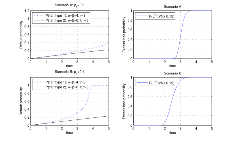
Figure 1: Conditional probabilities of default and excess loss probabilities in a portfolio of $N=125$ obligors where $L^{N}(t)$ is as defined in Section 2.2. Scenario A represents a portfolio where only the $20\%$ of obligors are of type 1 whereas in Scenario B $40\%$ of the obligors are of type 1. In both Scenario A and B we have $\lambda_{1}=[4,4,3]$, $\lambda_{2}=[0.1,0.1,3]$, where $\lambda_{i}$ describes the idiosyncratic characteristics of obligors of type $i=1,2$.

It may be argued that an approximation via an infinite portfolio may not reproduce the real situation. In Figure 2 we show a comparison between the evolution in time of the default probabilities in the two groups of obligors computed under $Q_{*}$ (in the upper part) and simulated via the real Markov process with $N=125$ (in the lower part). Here the parameters are $\lambda_{1}=(3,3,3)$, $\lambda_{2}=(0.1,0.1,1)$. These graphs show that the asymptotic equation is a good approximation for the Markov process even with $N=125$.

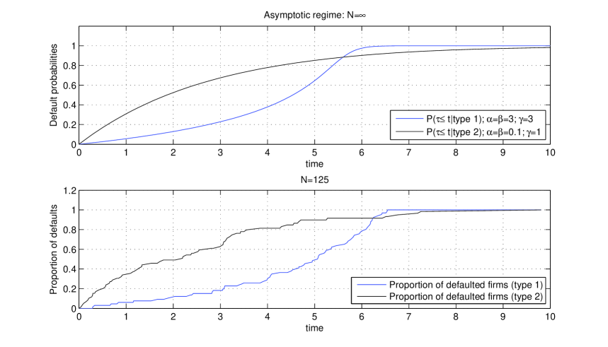
Figure 2: Comparison between the dynamics of the default probabilities of two groups of firms computed under two different models. In the upper part we see the plot under the asymptotic model with infinite firms (under $Q_{*}$). In the lowest one we have implemented a simulation of the Markov process directly (here $N=125$). The parameters are $\lambda_{1}=[3,3,3]$, $\lambda_{2}=[0.1,0.1,1]$, where $\lambda_{i}$ describes the idiosyncratic characteristics of obligors of type $i=1,2$. The distribution of $\lambda$ is in this case $\mu=\frac{1}{2}\delta_{\lambda_{1}}+\frac{1}{2}\delta_{\lambda_{2}}$.

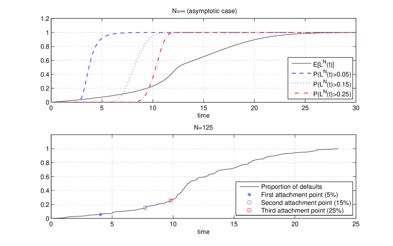
Figure 3: Evolution in time of the aggregate losses (in black) computed under two different models: under the asymptotic model (upper) and the Markov process (lower). The parameters are $\lambda_{1}=[2,6,4]$, $\lambda_{2}=[1,3,5]$, where $\lambda_{i}$ describes the idiosyncratic characteristics of obligors of type $i=1,2$. The distribution of $\lambda$ is in this case $\mu=0.4\delta_{\lambda_{1}}+0.6\delta_{\lambda_{2}}$.

Finally we show in Figure 3 the comparison between the evolution of the aggregate loss (in black) evaluated as before in two different ways. In the upper part we see the aggregate loss computed relying on Proposition 1. Below we see the plot of a trajectory of the Markov Process (with $N=125$). In the same graphs we have also plotted the dynamics of the probability of suffering a loss over certain thresholds $c_{k}$. In other words we plot $t\mapsto P(L^{N}(t)\geq c_{k})$ for $k=1,2,3$ (in this case $c_{1}=5\%,c_{2}=15\%,c_{3}=25\%$). Those probabilities are building blocks for computing the price of trances of CDO’s contracts. For a description of such a credit derivative see for instance [10].

3 Conclusions

We have proposed a model for credit contagion where heterogeneity and direct contagion among the firms are taken into account. We have then quantified the impact of contagion on the losses suffered by a financial institution holding a large portfolio with positions issued by the firms.

Compared to the existing literature on credit contagion, we have proposed a dynamic model where it is possible to describe the evolution of the indicators of financial distress. In this way we are able to compute the distribution of the losses in a large portfolio for any time horizon $T$, via a suitable version of the central limit theorem.

The peculiarity of our model is the fact that the homogeneity assumption is broken by introducing a random environment that makes it possible to take into account the idiosyncratic characteristics of the firms. One drawback of the intensity based models commonly proposed in the literature is the difficulty in managing large heterogeneous portfolios because of the presence of many obligors with different specifications. In this case it is common practice to assume homogeneity assumptions in order to reduce the complexity of the problem. A typical approach is to divide the portfolio into groups where the obligors may be considered exchangeable. We have shown that our model goes behind the identification of groups of firms that can be considered basically exchangeable. Despite this heterogeneity assumption our model has the advantage of being totally tractable: it is possible to compute in closed form the mean and the variance of a central limit type approximation for the losses due to a large portfolios in a dynamic fashion.

As an example of the general theory we have computed the default probabilities and different risk measures in a simple situation with only two groups of obligors. Moreover we have compared the numerical results obtained relying on the asymptotic model and on the central limit theorem (Corollary 2) with the results obtained in a simulation of the underlying Markov process with finite $N=125$. These results show the goodness of the approximation and are encouraging a more involved analysis. This issue is left to future research: it is in fact out of the scope of this work to pursue a punctual calibration of the model to real data.

Appendix A Proofs of main results

A.1 Proof of Theorem 1

We need to prove some technical lemmas.

Lemma 1

. Let $\mathcal{X}$ be a Polish space. Let $(P_{N})_{N}$ satisfy the LDP with rate $N$ and good rate function $H$. Let $F:\mathcal{X}\to\mathbb{R}$ be measurable, bounded from above and continuous on the set $\mathcal{X}_{H}:=\{x:H(x)<\infty\}$. Then the sequence of probability measures $(P^{F}_{N})_{N}$ defined by

$$\frac{dP^{F}_{N}}{dP_{N}}(\cdot)=\frac{\exp{(NF(\cdot))}}{\int_{\mathcal{X}}\exp{(NF(y))}P_{N}(dy)}$$ (A.1)

satisfies the LDP with the good rate function

$$I(x)=H(x)-F(x)-\inf_{y\in\mathcal{X}}[H(y)-F(y)].$$ (A.2)

In particular

$$\lim_{\,N\rightarrow+\infty}\frac{1}{N}\,\log\left[\int_{\mathcal{X}}\exp\left(NF(y)\right)P_{N}(dy)\right]=-\inf_{\,y\,\in\,\mathcal{X}}\left[H(y)-F(y)\right].$$ (A.2)

For a proof see [19]. This is a relaxed version of the usual Varadhan’s Lemma for tilted large deviations principles (see [20]). The statement is relaxed in the sense that we assume that a suitable function $F:\mathcal{X}\to\mathbb{R}$, instead of being continuous on all its domain, is continuous only on a subset $\mathcal{X}_{H}\varsubsetneq\mathcal{X}$ in the following sense:
For any sequence $(x_{n})_{n}\in\mathcal{X}$ such that $x_{n}\to x$, where $x\in\mathcal{X}_{H}$ we have $F(x_{n})\to F(x)$.
We point out that this is a stronger assumption than assuming continuity of the restriction of $F$ on the subset $\mathcal{X}_{H}$.

Lemma 2

. For given $\underline{\lambda}\in({\mathbb{R}}^{+}\times{\mathbb{R}}^{+}\times{\mathbb{R}})^{N}$,

$$\frac{dP^{\underline{\lambda}}_{N}}{dW^{\otimes N}}(\underline{y}[0,T])=\exp\{NF(\rho_{N}(\underline{y}[0,T],\underline{\lambda}))\}.$$ (A.3)

where $F(Q)$ has been defined in (1.2).

Proof.  It basically follows from the Girsanov formula for point processes (See [Br]).

$$\frac{dP^{\underline{\lambda}}_{N}}{dW^{\otimes N}}=\exp\left\{\sum_{i=1}^{N}\int_{0}^{T}\left[(1-y_{i}(t))-(1-y_{i}(t))e^{-\gamma_{i}+\beta_{i}\int\alpha^{\prime}\eta(t)\rho_{N}(d\eta[0,T],d\lambda^{\prime})}\right]dt+\right.$$

$$\hskip 28.45274pt+\left.\sum_{i=1}^{N}y_{i}(T){\left[-\gamma_{i}+\left(\beta_{i}\int\alpha^{\prime}\eta(t^{-})\rho_{N}(d\eta[0,T],d\lambda^{\prime})\right)\Big{|}_{t=\tau_{i}}\right]}\right\};$$

where $\tau_{i}$ has been defined in (1.2).
The term in the $\{\ \}$-brackets is exactly $F(Q)_{|Q=\rho_{N}}$ multiplied by $N$.  

We now define for each $Q\in{\cal{M}}$ and $t\in[0,T]$

$$m_{Q}(t):=\int\alpha\eta(t)Q(d\eta[0,T],d\lambda).$$ (A.4)

We shall often use this notation in the rest of this appendix.

Lemma 3

. F(Q) is bounded on ${\cal{M}}_{1}$ and continuous on the subset ${\cal{M}}_{A}:=\{Q\in{\cal{M}}_{1}:Q\ll W\otimes\mu\}$

Proof.  We rewrite $F(Q)$ as given in (1.2) using the notation introduced in (A.4).

$$F(Q)=\int Q(dy[0.T],d\lambda)\left\{\int_{0}^{T}(1-y(t))\left(1-e^{-\gamma}e^{\beta m_{Q}(t)}\right)dt\right.\\ +\left.y(T)\left[-\gamma+\beta m_{Q}(t^{-})\Big{|}_{t=\tau(y[0,T])}\right]\right\},$$ (A.4)

The argument in the $\{\ \}$-brackets is bounded, thus we are allowed to interchange the expectation with respect to $Q$ and the time integral.

$$F(Q)=\int_{0}^{T}E^{Q}\left[1-y(t)\right]\ dt-\int_{0}^{T}E^{Q}\left[e^{-\gamma}e^{\beta m_{Q}(t)}\ (1-y(t))\right]\ dt-\\ -E^{Q}\left[\gamma y(T)\right]+E^{Q}\left[\beta y(T)m_{Q}(t^{-})\Big{|}_{t=\tau(y[0,T])}\right].$$

We show now boundedness and continuity of $F$. The boundedness is easily proved since $y\in\{0;1\}$, and the distribution of $\lambda$ under $Q\in{\cal{M}}_{1}^{b}$ has bounded support.
In order to prove the continuity on $\mathcal{M}_{A}$, we consider a sequence of probabilities $(Q_{n})_{n\geq 0}\in\mathcal{M}_{1}^{b}$ converging weakly to $Q\in\mathcal{M}_{A}$. We split the proof in different steps.
We show first that

$$\lim_{n}E^{Q_{n}}[f(\lambda)y(t)]=E^{Q}[f(\lambda)y(t)]$$ (A.5)

for all $t\in[0,T]$ and for any continuous function $f:\mathbb{R}^{+}\times\mathbb{R}^{+}\times\mathbb{R}\to\mathbb{R}$ bounded on the support of $\mu$. This statement is not trivial, since the projection $y{[0,T]}\to y(t)$ is not continuous in ${\cal{D}}[0,T]$. However, define for any $\epsilon>0$ the functions

$$g^{-}_{t}(\epsilon;f):=\frac{1}{\epsilon}\int_{t-\epsilon}^{t}f(\lambda)y(s)ds\ ,\qquad g^{+}_{t}(\epsilon;f):=\frac{1}{\epsilon}\int_{t}^{t+\epsilon}f(\lambda)y(s)ds;$$

where we suppose that the trajectory $y[0,T]$ can be extended to the larger interval $[0-\epsilon,\ T+\epsilon]$ by continuity.
These functions are continuous in ${\cal{D}}[0,T]$, bounded by $\|f\|_{\infty}$ for any $\epsilon$ and such that $g^{-}_{t}(\epsilon;f)\leq f(\lambda)y(t)\leq g^{+}_{t}(\epsilon;f)$ a.s. for any $t$. Thus, by the Lebesgue convergence theorem,

$$\limsup_{n}E^{Q_{n}}[f(\lambda)y(t)]\leq\lim_{n}E^{Q_{n}}[g^{+}(\epsilon;f)]=E^{Q}[g^{+}(\epsilon;f)],\quad\forall\epsilon>0.$$

Letting $\epsilon\to 0$ and noticing that $\lim_{\epsilon\to 0}g^{+}_{t}(\epsilon;f)=f(\lambda)y(t)$ we get

$$\limsup_{n}E^{Q_{n}}[f(\lambda)y(t)]\leq E^{Q}[f(\lambda)y(t)].$$

The same argument holds for $g^{-}_{t}(\epsilon;f)$; here $\lim_{\epsilon\to 0}g^{-}_{t}(\epsilon;f)=f(\lambda)y(t^{-})$. Thus

$$E^{Q}[f(\lambda)y(t^{-})]\leq\liminf_{n}E^{Q_{n}}[f(\lambda)y(t)]\leq\limsup_{n}E^{Q_{n}}[f(\lambda)y(t)]\leq E^{Q}[f(\lambda)y(t)].$$

Notice that $f(\lambda)y(t)$ and $f(\lambda)y(t^{-})$ may differ only on the event $\{y(t^{-})\neq y(t)\}$. But this event has measure zero for any $Q\in\mathcal{M}_{A}$, since $(W\otimes\eta)(\{y(t^{-})\neq y(t)\})=0$. This implies that the corresponding expected values must coincide; as a consequence $E^{Q}[f(\lambda)y(t)]-E^{Q}[f(\lambda)y(t^{-})]=0$. We have thus proved that

$$\lim_{n}E^{Q_{n}}[f(\lambda)y(t)]=E^{Q}[f(\lambda)y(t)]\ \ \mbox{for all}\ t.$$ (A.6)

Notice that in saying that $(W\otimes\eta)(\{y(t^{-})\neq y(t)\})=0$ we have used the fact that the distribution function of $\tau$ under $W\otimes\eta$ is exponential. In particular, it is absolutely continuous. A similar argument shows that if $Q\notin{\cal{M}}_{A}$ then $E^{Q_{n}}[y(t)]$ converges pointwise in $t$ to $E^{Q}[y(t)]$, for all those $t$ such that $Q(\tau=t)=0$.
Taking $f(\lambda)\equiv 1$ we simply have that for all $t$, $E^{Q}[y(t)]$ is a continuous mapping in $Q$ on $\mathcal{M}_{A}$. Choosing instead $f(\lambda)=e^{-\gamma}$, $f(\lambda)=-\gamma$ and $f(\lambda)=\alpha$, we prove continuity for $E^{Q}\left[y(t)\ e^{-\gamma}\right]$, $E^{Q}\left[-\gamma y(T)\right]$ and $m_{Q}(t)$ respectively.
The next step is to show that $Q_{n}\to Q$ implies that

$$\left|E^{Q}\!\left[\int_{0}^{T}(1-y(t))\ e^{-\gamma}e^{\beta m_{Q}(t)}dt\right]\!-E^{Q_{n}}\!\left[\int_{0}^{T}(1-y(t))\ e^{-\gamma}e^{\beta m_{Q_{n}}(t)}dt\right]\right|$$ (A.7)

converges to zero.

We add and subtract $E^{Q_{n}}\left[\int_{0}^{T}(1-y(t))\ e^{-\gamma}e^{\beta m_{Q}(t)}dt\right]$ :

$$\left|E^{Q}\left[\int_{0}^{T}(1-y(t))\ e^{-\gamma}e^{\beta m_{Q}(t)}dt\right]-E^{Q_{n}}\left[\int_{0}^{T}(1-y(t))\ e^{-\gamma}e^{\beta m_{Q}(t)}dt\right]+\right.$$

$$+\left.E^{Q_{n}}\left[\int_{0}^{T}\left((1-y(t))\ e^{-\gamma}\right)\left(e^{\beta m_{Q}(t)}-e^{\beta m_{Q_{n}}(t)}\right)dt\right]\right|\leq|a_{n}|+|b_{n}|$$

where

$$a_{n}=E^{Q}\left[\int_{0}^{T}(1-y(t))\ e^{-\gamma}e^{\beta m_{Q}(t)}dt\right]-E^{Q_{n}}\left[\int_{0}^{T}(1-y(t))\ e^{-\gamma}e^{\beta m_{Q}(t)}dt\right];$$

$$b_{n}=E^{Q_{n}}\left[\int_{0}^{T}\left((1-y(t))\ e^{-\gamma}\right)\left(e^{\beta m_{Q}(t)}-e^{\beta m_{Q_{n}}(t)}\right)dt\right].$$

$|a_{n}|$ goes to zero by weak convergence.

Concerning $b_{n}$ we see that

$$|b_{n}|\leq\int_{0}^{T}E^{Q_{n}}\left[(1-y(t))\ e^{-\gamma}\cdot\left|e^{\beta m_{Q}(t)}-e^{\beta m_{Q_{n}}(t)}\right|\right]dt\leq$$

$$\leq\int_{0}^{T}E^{Q_{n}}\left[(1-y(t))\ e^{-\gamma}\cdot\left|e^{\beta m_{Q}(t)}-e^{\beta m_{Q_{n}}(t)}\right|\right]dt.$$

We now show that

$$E^{Q_{n}}\left[(1-y(t))\ e^{-\gamma}\cdot\left|e^{\beta m_{Q}(t)}-e^{\beta m_{Q_{n}}(t)}\right|\right]\to 0.$$

We can rewrite it as

$$E^{Q_{n}}\left[(1-y(t))\ e^{-\gamma}e^{\beta m_{Q}(t)}\cdot\left|e^{\beta\left[m_{Q}(t)-m_{Q_{n}}(t)\right]}-1\right|\right]\leq$$

$$\leq KE^{Q_{n}}\left[\left|e^{\beta\left[m_{Q}(t)-m_{Q_{n}}(t)\right]}-1\right|\right]=(*)$$

for a suitable $K\in\mathbb{R}^{+}$, where we have used the fact that $(1-y(t))\ e^{-\gamma}e^{\beta m_{Q}(t)}$ is uniformly bounded. We now look at the term into the expectation

$$\left|e^{\beta\left[m_{Q}(t)-m_{Q_{n}}(t)\right]}-1\right|\leq K_{2}|m_{Q}(t)-m_{Q_{n}}(t)|$$

again by uniformly boundedness, for a suitable $K_{2}$. Thus

$$(*)\leq K_{3}|m_{Q}(t)-m_{Q_{n}}(t)|,$$

and this converges to zero thanks to what we have shown in (A.5).
As a consequence, $|b_{n}|$ goes to zero as well, since we are allowed to interchange the limit and the time integral, by dominated convergence.

It remains to show the continuity of the term

$$E^{Q}[\beta y(T)m_{q}(\tau^{-})].$$ (A.8)

Indeed, take a sequence $Q_{n}\to Q$, $Q\in{\cal{M}}_{A}$, then

$$\left|E^{Q_{n}}[\beta y(T)m_{Q_{n}}(\tau^{-})]-E^{Q}[\beta y(T)m_{Q}(\tau^{-})]\right|\\ \leq\left|E^{Q_{n}}[\beta y(T)\left\{m_{Q_{n}}(\tau^{-})-m_{Q}(\tau^{-})\right\}]\right|+\left|E^{Q_{n}}[\beta y(T)m_{Q}(\tau^{-})]-E^{Q}[\beta y(T)m_{Q}(\tau^{-})]\right|.$$

The second term goes to zero by weak convergence since the function $m_{Q}$ is continuous. Concerning the first term, it is enough to show that $\left\{m_{Q_{n}}(t)-m_{Q}(t)\right\}$ converges to zero uniformly on $[0,T]$. To show this, we fix $t\in[0,T]$ then the following facts hold true:

• For $\delta_{1}>0$ there exists $\epsilon>0$ such that $|s-t|\leq\epsilon\Rightarrow|m_{Q}(s)-m_{Q}(t)|\leq\delta_{1}$

• There exists $\bar{n}$ such that $\forall n\geq\bar{n}$
  $|m_{Q_{n}}(t+\epsilon)-m_{Q}(t+\epsilon)|\leq\delta_{2}\ ;\ \$ $|m_{Q_{n}}(t-\epsilon)-m_{Q}(t-\epsilon)|\leq\delta_{3}$

Point $(a)$ is due to the continuity of $m_{Q}(t)$ for $Q\in{\cal{M}}_{A}$ whereas $(b)$ follows by the fact that $m_{Q_{n}}(t)\to m_{Q}(t)$ pointwise in $t$ as shown in (A.5). Notice that when $t+\epsilon>T$ or $t-\epsilon<0$ the inequalities in $(b)$ are modified appropriately without loss of generality.
We now claim that fixing $s\in O_{t}:=[t-\epsilon,\ t+\epsilon]$ we have

$$|m_{Q_{n}}(s)-m_{Q}(s)|\leq\delta_{1}+\delta_{2}+\delta_{3}=\bar{\delta}.$$ (A.9)

Fix $s$ and $n$ and suppose $m_{Q_{n}}(s)\leq m_{Q}(s)$ (the other case is treated in the same way):

$$m_{Q}(s)-m_{Q_{n}}(s)\leq m_{Q}(t+\epsilon)-m_{Q}(t-\epsilon)+m_{Q}(t-\epsilon)-m_{Q_{n}}(t-\epsilon)\leq\delta_{1}+\delta_{3};$$

where we have used the fact that $m_{Q}(t)$ is increasing in $t$ for all $Q\in{\cal{M}}_{1}$. Thus we can extract a finite covering $\{O_{t_{k}}\}$ of $[0,T]$ where (A.9) holds true hence uniform convergence is proved.  

Proof of Theorem 1.
We denote by ${\cal{P}}_{N}$ the distribution of $\rho_{N}$ under $P_{N}$, i.e. ${\cal{P}}_{N}:=P^{N}\circ\rho_{N}^{-1}$. We now state a LDP for the sequence $\{{\cal{P}}_{N}\}_{N}$. Thanks to Lemma 2, we have identified the Radon Nikodym derivative that relates $W^{\otimes N}$ and $P^{\underline{\lambda}}_{N}$ (where $W^{\otimes N}$ plays the role of the reference measure). A natural way to develop a large deviation principle is now to rely on Lemma 1.

Since $(y_{i}[0,T];\lambda_{i})$ are i.i.d. random variables under $(W\otimes\mu)^{\otimes N}$, we can apply Sanov’s Theorem (see [20]) to the sequence of measures $(\mathcal{W}_{N})_{N}$, where $\mathcal{W}_{N}$ represents the law of the empirical measure in the case of independence (i.e. under $(W\otimes\mu)^{\otimes N}$). Hence $(\mathcal{W}_{N})_{N}$ obeys a large deviation principle with rate function $H(Q|W\otimes\mu)$.
Being $F(Q)$ bounded in the weak topology and continuous on ${\cal{M}}_{A}\supset{\cal{M}}_{H}$ where $\mathcal{M}_{A}=\{Q\in{\cal{M}}_{1}|Q\ll W\otimes\mu\}$ and $\mathcal{M}_{H}=\{Q\in{\cal{M}}_{1}:H(Q|W\otimes\mu)<\infty\}$, we can rely on Lemma 1 to conclude that the sequence $(\mathcal{P}_{N})_{N}$ obeys a large deviation principle with good rate function

$$I(Q)=H(Q|W\otimes\mu)-F(Q)-\inf_{R\in{\cal{M}}_{1}}[H(R|W\otimes\mu)-F(R)].$$

We finish the proof by showing that

$$\inf_{R\in{{\cal{M}}}_{1}}[H(R|W\otimes\mu)-F(R)]=\lim_{N\to\infty}\frac{1}{N}\log\left[\int_{{\cal{M}}_{1}}e^{NF(Q)}\mathcal{W}_{N}(dQ)\right]=0.$$ (A.10)

The first equality is simply a consequence of Equation (A.2).
We are thus left to prove that $\int_{{\cal{M}}_{1}}e^{NF(Q)}\mathcal{W}_{N}(dQ)=1$. Indeed,

$$\mathcal{P}_{N}(\,\cdot\ )=\int\mu^{\otimes N}(d\underline{\lambda})P^{\underline{\lambda}}_{N}(\rho_{N}\in\cdot\ )=$$

$$=\int\mu^{\otimes N}(d\underline{\lambda})\int\mathbb{I}_{\{\rho_{N}\in\cdot\ \}}\frac{dP^{\underline{\lambda}}_{N}}{dW^{\otimes N}}dW^{\otimes N}=\int\mathbb{I}_{\{\rho_{N}\in\cdot\ \}}e^{NF(\rho_{N})}\ d(W^{\otimes N}\otimes\mu^{\otimes N})=$$

$$=\int\mathbb{I}_{\{Q\in\cdot\ \}}e^{NF(Q)}\mathcal{W}_{N}(dQ).$$

Being $\mathcal{P}_{N}({\mathcal{M}}_{1})=1$, the thesis follows. 

A.2 Proof of Theorem 2

We need to define a new process and a technical lemma related to it.
We associate with any $Q\in{\cal{M}}_{1}$ the law of a time inhomogeneous Markov process on $\{0;1\}$ which evolves according to the following rules:

$$\begin{array}[]{llc}y=0\to y=1&\mbox{with intensity}&e^{-\gamma}e^{\beta\int\alpha^{\prime}\eta(t)Q(d\eta[0,T],d\lambda)}\\ y=1\to y=0&\mbox{with intensity}&0\end{array}$$

and with $y_{i}(0)=1$ for all $i=1,...,N$.
We denote by $P^{\lambda,Q}$ the law of this process and by $P^{Q}=P^{\lambda,Q}\otimes\eta$. In other words, $P^{\lambda,Q}$ is the law of the Markov process on $\{0;1\}$ with initial distribution $\delta_{0}$ and time-dependent generator $L^{\lambda,Q}_{t}$ defined as

$$L^{\lambda,Q}_{t}f(s)=(1-s)e^{-\gamma}e^{\beta\int\alpha^{\prime}\eta(t)Q(d\eta[0,T],d\lambda)}(f(1-s)-f(s)).$$ (A.11)

We show now an important property of $P^{Q}$.

Lemma 4

. For every $Q\in{\cal{M}}_{1}$, we have

$$I(Q)=H(Q|P^{Q}).$$

Proof.  We distinguish two cases:
Case 1. $Q:H(Q|W\otimes\eta)<\infty$. We have

$$I(Q)=\int\log\frac{dQ}{d(W\otimes\eta)}dQ-F(Q).$$

By Girsanov’s formula for continuous time Markov chains, we obtain

$$\log\frac{dP^{\lambda,Q}}{dW}=\int_{0}^{T}(1-y(t))\left(1-e^{-\gamma}e^{\beta\int Q(d\eta[0,T],d\lambda^{\prime})\alpha^{\prime}\eta(t)}\right)dt\\ +y(T)\left[-\gamma+\left(\beta\int\alpha^{\prime}\eta(t^{-})Q(d\eta[0,T],d\lambda^{\prime})\right)\Big{|}_{t=\tau(y[0,T])}\right];$$ (A.11)

hence, by definition of $F$ given in (1.2) we have

$$F(Q)=\int\log\frac{dP^{\lambda,Q}}{dW}\ dQ$$

so that

$$I(Q)=\int\log\frac{dQ}{d(W\otimes\eta)}dQ-\int\log\frac{dP^{\lambda,Q}}{dW}dQ=\int\log\frac{dQ}{dP^{Q}}dQ$$ (A.12)

where the last equality follows from

$$\frac{dQ}{d(W\otimes\eta)}\frac{dW}{dP^{\lambda,Q}}=\frac{dQ}{d(W\otimes\eta)}\frac{d(W\otimes\eta)}{dP^{Q}}=\frac{dQ}{dP^{Q}}.$$

Being $\int\log\frac{dQ}{dP^{Q}}dQ=H(Q|P^{Q})$, the thesis follows.

Case 2. $Q:H(Q|W\otimes\eta)=+\infty$. In this case $I(Q)=+\infty$.
Thus we have to check that $H(Q|P^{Q})=+\infty$ as well. Being

$$H(Q|P^{Q})=\int\log\frac{dQ}{d(W\otimes\eta)}dQ+\int\log\frac{dW}{dP^{\lambda,Q}}dQ,$$

the thesis follows since $\int\log\frac{dQ}{d(W\otimes\eta)}dQ=+\infty$ being $H(Q|W\otimes\eta)=+\infty$ and since $\int\log\frac{dW}{dP^{\lambda,Q}}dQ=-F(Q)$ which is bounded .  

Proof of Theorem 2.
By properness of the relative entropy ($H(\mu|\nu)=0\Rightarrow\mu=\nu$), from Lemma A.11 we have that the equation $I(Q)=0$ is equivalent to $Q=P^{Q}$. Suppose $\bar{Q}$ is a solution of this last equation. In this case $\bar{Q}=P^{\bar{Q}}=P^{\lambda,\bar{Q}}\otimes\mu$, where $P^{\lambda,\bar{Q}}$ is the law of the Markov process on $\{0;1\}$ with initial distribution $\delta_{0}$ and time-dependent generator $L^{\lambda,\bar{Q}}_{t}$ as defined in (A.11). The marginals of a Markov process are solutions of the corresponding forward equation. This leads to the fact that $\bar{q}_{t}:=\Pi_{t}P^{\lambda,\bar{Q}}$, the $t-$projection of $P^{\lambda,\bar{Q}}$, is a solution of $\dot{q}_{t}=\mathcal{L}_{t}^{\lambda,\bar{Q}}$ where $\mathcal{L}_{t}^{\lambda,\bar{Q}}$ is the adjoint of $L_{t}^{\lambda,Q}$:

$$(\mathcal{L}^{\lambda,\bar{Q}}_{t}q)(x)=xe^{-\gamma}e^{\beta\int\alpha^{\prime}\eta(t)\bar{Q}(d\eta[0,T],d\lambda^{\prime})}q(-x)-\mathbb{(}1-x)e^{-\gamma}e^{\beta\int\alpha^{\prime}\eta(t)\bar{Q}(d\eta[0,T],d\lambda^{\prime})}q(x).$$

More specifically, when $x=0$ we have

$$(\mathcal{L}^{\lambda,\bar{Q}}_{t}q)(0)=-e^{-\gamma}e^{\beta\int\alpha^{\prime}\eta(t)\bar{Q}(d\eta[0,T],d\lambda^{\prime})}q(0)$$

and when $x=1$

$$(\mathcal{L}^{\lambda,\bar{Q}}_{t}q)(1)=e^{-\gamma}e^{\beta\int\alpha^{\prime}\eta(t)\bar{Q}(d\eta[0,T],d\lambda^{\prime})}q(0).$$ (A.13)

We now prove that $\dot{q}_{t}=\mathcal{L}^{\lambda,\bar{Q}}_{t}q$ admits at most one solution for each initial condition. To see this, define $\bar{q}_{t}(\lambda):=P^{\lambda,\bar{Q}}(y(t)=1)$. Then $\frac{d\bar{q}_{t}(\lambda)}{dt}=G(\bar{q}_{t}(\lambda))$, where $G(q)=e^{-\gamma}e^{\beta\int\alpha^{\prime}q(\lambda^{\prime})\mu(d\lambda^{\prime})}(1-q(\lambda))$. Notice that $\bar{q}_{t}(\lambda)\in L^{1}(\mu)$ and $G(\cdot)$ is a locally Lipschitz operator on a Banach space. Thus $\frac{d\bar{q}_{t}(\lambda)}{dt}=G(\bar{q}_{t}(\lambda))$ has at most one solution in $[0,T]$, for a given initial condition (see [2], Theorem VII.3).
Since $P^{\bar{Q}}$ is totally determined by the flow $\bar{q}_{t}$, it follows that equation $Q=P^{Q}$ has at most one solution. The existence of a solution follows from the fact that $I(Q)$ is the rate function of a LDP, and therefore must have at least one zero. By what shown in (A.13), $\bar{q}_{t}(\lambda)$ solves (1.3). Hence $Q_{*}$ turns out to be the unique solution of the fixed point argument $Q=P^{Q}$. Moreover, it satisfies all the conditions of Theorem 2.  

A.3 Proof of Theorem 3

The key technical tool for the proof of Theorem 3 is the following result due to Bolthausen [3].

Theorem 4

. Let $(B,\|\cdot\|)$ be a real separable Banach space. Let $(Z_{k})_{k\geq 1}$ be a sequence of $B$-valued, i.i.d. random variables, defined on the probability space $(\Omega,\mathcal{A},\mathbb{P})$ and denote by $w$ their common law. Define $X_{N}:=\frac{1}{N}\sum_{k=1}^{N}Z_{k}$ and consider a continuous map $\Psi:B\to\mathbb{R}$. Suppose that the following conditions are satisfied:

• $\int\exp(r|x|)w(dx)<\infty$   for all $r\in\mathbb{R}$.

• For any $x\in B$, $\Psi(x)\leq C_{1}+C_{2}\|x\|$, for some $C_{1},C_{2}>0$. Moreover, $\Psi$ is three times continuously Fréchet differentiable.

• Define, for $h\in B^{\prime}$ (the topological dual of $B$), $\Lambda(h):=\int e^{h(z)}w(dz)$, and for $x\in B$, $\Lambda^{*}(x):=\sup_{h\in B^{\prime}}[h(x)-\Lambda(h)]$. Assume that there exists a unique $z^{*}\in B$ such that $\Lambda^{*}(z^{*})-\Psi(z^{*})=\inf_{z\in B}[\Lambda^{*}(z)-\Psi(z)]$.

• Define the probability $p$ on $B$ by $\frac{dp}{dw}=\frac{e^{D\Psi(z_{*})}}{c}$ for a suitable normalizing factor $c$. This probability is well defined and $\int zp(dz)=z^{*}$. Let $p_{*}$ denote the centered version of $p$, i.e., $p_{*}=p\circ\theta_{x^{*}}^{-1}$, where $\theta_{a}:B\to B$ is defined by $\theta_{a}(x)=x-a$. For $h\in B^{\prime}$ define $\tilde{h}\in B$ by $\tilde{h}=\int zh(z)p_{*}(dz)$. Then we assume that for every $h\in B^{\prime}$ such that $\tilde{h}\neq 0$

  $$\int h^{2}(z)p_{*}(dz)-D^{2}\Psi(z^{*})[\tilde{h},\tilde{h}]>0.$$

• $B$ is a Banach space of type 2.

Now, letting $\pi_{N}$ be the probability on $(\Omega,\mathcal{A})$ given by

$$\frac{d\pi_{N}}{d\,\mathbb{P}}=\frac{e^{N\left(\Psi(X_{N})+\frac{\Sigma(X_{N})}{N}\right)}}{E^{\mathbb{P}}\left[e^{N\left(\Psi(X_{N})+\frac{\Sigma(X_{N})}{N}\right)}\right]}\ ,$$ (A.14)

where $\Sigma$ is linear, continuous and bounded on the support of the law of $X_{N}$, uniformly in $N$. Then, for every $h_{1},...,h_{n}\in B^{\prime}$, the $\pi_{N}$-law of the $n-$dimensional vector

$$\sqrt{N}\left(h_{i}(X_{N})-h_{i}(z_{*})\right)_{i=1}^{n}$$

converges weakly, as $N\to\infty$, to the law of a centered Gaussian vector with covariance matrix $\mathcal{C}\in\mathbb{R}^{n\times n}$, such that for $i,j=1,...,n$

$$(\mathcal{C})_{i,j}=\int h_{i}(z)h_{j}(z)p_{*}(dz)-D^{2}\Psi(z_{*})[\tilde{h}_{i},\tilde{h}_{j}].$$ (A.15)

Remark 2

.

• The Theorem in [3] is stated for $\Sigma=0$. The same proof applies with our assumptions on $\Sigma$ without changes. It is likely that these assumptions can be weakened considerably.

• The Theorem in [3] contains a stronger statement that the one given here. Indeed, it is shown that the field $\sqrt{N}\left(h(X_{N})-h(z_{*})\right)_{h\in B^{\prime}}$ converges weakly to a Gaussian field, while we only stated convergence for finite dimensional distributions. This is all we need to prove Theorem 3. Our proof has not allowed to take advantage of the full strength of the Theorem in [3].

The “natural” space for the Central Limit Theorem in Theorem 3 is the set ${\cal{M}}$ of signed measures, which is not a Banach space. To apply Theorem 4, we need to map ${\cal{M}}$ to a Banach space of type 2.

Lemma 5

. The following properties hold true under the reciprocity condition (R):

• There exists a Banach space of type $2$ $(B,\|\cdot\|)$, a linear map $T:\mathcal{M}\to B$, continuous on the set $\{Q:Q(\tau=T)=0\}$. Moreover there exist two continuous maps $\Psi,\Sigma:B\to\mathbb{R}$, where $\Psi$ is bounded and three times Fréchet differentiable and $\Sigma$ is linear, such that

  $$\frac{dP^{\lambda}_{N}}{dW^{\otimes N}}=\exp\left\{N\left[\Psi(T(\rho_{N}))+\frac{\Sigma(T(\rho_{N}))}{N}\right]\right\}\ ,\qquad a.s.$$ (A.16)

• For any vector $\Phi=(\Phi_{1},...,\Phi_{n})\in{\mathcal{C}_{b}}^{n}$ there exist $h=(h_{1},...,h_{n})\subset B^{\prime}$ such that $(h_{i}\circ T)(Q)=\int\Phi_{i}dQ$, where $B^{\prime}$ stands for the topological dual of $B$.

Proof.  The first step consists in giving an alternative expression for $F(Q)$ given in (1.2). Look at the term

$$\int Q(dy[0,T],d\lambda)\left\{y(T)\left(\beta\int Q(d\eta[0,T],d\lambda^{\prime})\alpha^{\prime}\eta(t^{-})\right)\Big{|}_{t=\tau(y[0,T])}\right\}.$$

using the reciprocity condition (R), we obtain

$$b\int Q(dy[0,T],d\lambda)\left\{y(T)\alpha\int Q(d\eta[0,T],d\lambda^{\prime})\alpha^{\prime}\eta(t^{-})\Big{|}_{t=\tau(y[0,T])}\right\}\\ =b\int Q(dy[0,T],d\lambda)Q(d\eta[0,T],d\lambda^{\prime})\alpha\alpha^{\prime}{\bf 1}_{\{\tau(y[0,T])\leq T\}}{\bf 1}_{\{\tau(\eta[0,T])<\tau(y[0,T])\}}=(*)$$

Note that ${\bf 1}_{\{\tau(\eta[0,T])<\tau(y[0,T])\}}={\bf 1}_{\{\tau(\eta[0,T])\leq T\}}$ unless $\tau(y[0,T])\leq\tau(\eta[0,T])\leq T$. Thus

$$(*)=b\int Q(dy[0,T],d\lambda)Q(d\eta[0,T],d\lambda^{\prime})\alpha\alpha^{\prime}{\bf 1}_{\{\tau(y[0,T])\leq T\}}{\bf 1}_{\{\tau(\eta[0,T])\leq T\}}\\ -b\int Q(dy[0,T],d\lambda)Q(d\eta[0,T],d\lambda^{\prime})\alpha\alpha^{\prime}{\bf 1}_{\{\tau(\eta[0,T])\leq T\}}{\bf 1}_{\{\tau(y[0,T])\leq\tau(\eta[0,T])\}}\\ =b\int Q(dy[0,T],d\lambda)Q(d\eta[0,T],d\lambda^{\prime})\alpha\alpha^{\prime}{\bf 1}_{\{\tau(y[0,T])\leq T\}}{\bf 1}_{\{\tau(\eta[0,T])\leq T\}}\\ -b\int Q(dy[0,T],d\lambda)Q(d\eta[0,T],d\lambda^{\prime})\alpha\alpha^{\prime}{\bf 1}_{\{\tau(\eta[0,T])\leq T\}}{\bf 1}_{\{\tau(y[0,T])<\tau(\eta[0,T])\}}\\ -b\int Q(dy[0,T],d\lambda)Q(d\eta[0,T],d\lambda^{\prime})\alpha\alpha^{\prime}{\bf 1}_{\{\tau(\eta[0,T])\leq T\}}{\bf 1}_{\{\tau(y[0,T])=\tau(\eta[0,T])\}}.$$

Therefore

$$b\int Q(dy[0,T],d\lambda)\left\{y(T)\alpha\int Q(d\eta[0,T],d\lambda^{\prime})\alpha^{\prime}\eta(t^{-})\Big{|}_{t=\tau(y[0,T])}\right\}\\ =\frac{b}{2}\int Q(dy[0,T],d\lambda)Q(d\eta[0,T],d\lambda^{\prime})\alpha\alpha^{\prime}{\bf 1}_{\{\tau(y[0,T])\leq T\}}{\bf 1}_{\{\tau(\eta[0,T])\leq T\}}\\ -\frac{b}{2}\int Q(dy[0,T],d\lambda)Q(d\eta[0,T],d\lambda^{\prime})\alpha\alpha^{\prime}{\bf 1}_{\{\tau(\eta[0,T])\leq T\}}{\bf 1}_{\{\tau(y[0,T])=\tau(\eta[0,T])\}}\\ =\frac{b}{2}\left[\int Q(dy[0,T],d\lambda)\alpha{\bf 1}_{\{\tau(y[0,T])\leq T\}}\right]^{2}-\frac{b}{2}\sum_{t\in[0,T]}\left[\int Q(dy[0,T],d\lambda)\alpha{\bf 1}_{\{\tau(y[0,T])=t\}}\right]^{2}.$$

Thus, defining

$$F_{1}(Q):=\int Q(dy[0,T],d\lambda)\left\{\int_{0}^{T}(1-y(t))\left(1-e^{-\gamma}e^{\beta\int Q(d\eta[0,T],d\lambda^{\prime})\alpha^{\prime}\eta(t)}\right)dt-\gamma y(T)\right\}\\ +\frac{b}{2}\left[\int Q(dy[0,T],d\lambda)\alpha y(T)\right]^{2}$$ (A.17)

and

$$F_{2}(Q):=-\frac{b}{2}\sum_{t\in[0,T]}\left[\int Q(dy[0,T],d\lambda)\alpha{\bf 1}_{\{\tau(y[0,T])=t\}}\right]^{2},$$ (A.18)

we have that $F(Q)=F_{1}(Q)+F_{2}(Q)$. Lemma 2 thus holds also after replacing $F$ by $F_{1}+F_{2}$. Let $M>0$ be a constant such that, under $\eta$, the random parameters $\alpha$ and $\gamma$ have absolute value less that $M/2$. Now we define the following maps:

$$T_{1}:\begin{array}[]{rcl}{\cal{M}}&\rightarrow&L^{2}[0,T]\\ Q&\mapsto&\frac{1}{2}\int Q(dy[0,T],d\lambda)[1-y(t)]\end{array}$$

$$T_{2}:\begin{array}[]{rcl}{\cal{M}}&\rightarrow&L^{2}([0,T]\times{\mathbb{N}})\\ Q&\mapsto&C(M)\int Q(dy[0,T],d\lambda)\left[e^{-\gamma}\frac{(M\beta)^{n}}{n!}(1-y(t))\right]\end{array}$$

$$T_{3}:\begin{array}[]{rcl}{\cal{M}}&\rightarrow&L^{2}[0,T]\\ Q&\mapsto&\int Q(dy[0,T],d\lambda)\frac{\alpha}{M}y(t)\end{array}$$

$$T_{4}:\begin{array}[]{rcl}{\cal{M}}&\rightarrow&{\mathbb{R}}\\ Q&\mapsto&\int Q(dy[0,T],d\lambda)\frac{\gamma}{M}y(T)\end{array}$$

$$T_{5}:\begin{array}[]{rcl}{\cal{M}}&\rightarrow&{\mathbb{R}}\\ Q&\mapsto&\int Q(dy[0,T],d\lambda)\frac{\alpha}{M}y(T)\end{array}$$

$$T_{6}:\begin{array}[]{rcl}{\cal{M}}&\rightarrow&{\mathbb{R}}\\ Q&\mapsto&\int Q(dy[0,T],d\lambda)\alpha^{2}y(T)\end{array},$$

where $C(M)$ is some positive constant such that $C(M)e^{-\gamma}e^{M\beta}\leq\frac{1}{2}$ $\eta$ almost surely. Note that, for $Q\in{\cal{M}}_{1}$ and $i=1,2,\ldots,5$, we have that $|T_{i}(Q)|\leq\frac{1}{2}$. Now, let $g:{\mathbb{R}}\rightarrow{\mathbb{R}}$ be a ${\cal{C}}^{\infty}$ function such that $g(x)=x$ for $|x|\leq 1/2$, $g(x)=0$ for $|x|>3/4$ and $\|g\|_{\infty}\leq 3/4$. For

$$z=(z_{1},z_{2},z_{3},z_{4},z_{5},z_{6})\in L^{2}[0,T]\times L^{2}([0,T]\times{\mathbb{N}})\times L^{2}[0,T]\times R\times R\times R$$

we set

$$\Psi(z):=2\int_{0}^{T}g(z_{1}(t))dt-\frac{1}{C(M)}\sum_{n}\int_{0}^{T}g((z_{2}(t,n))g(z_{3}(t))^{n}dt-Mg(z_{4})+\frac{bM^{2}}{2}g^{2}(z_{5})$$ (A.19)

and

$$\Sigma(z):=-\frac{b}{2}z_{6}.$$ (A.20)

We now claim that, for $Q\in{\cal{M}}_{1}$ and setting $T=(T_{1},T_{2},T_{3},T_{4},T_{5},T_{6})$,

$$F_{1}(Q)=\Psi(T(Q)).$$ (A.21)

Moreover

$$F_{2}(\rho_{N})=\frac{\Sigma(T(\rho_{N}))}{N},\quad W\otimes\mu-a.s.$$ (A.22)

so that (A.16) holds. Equation (A.21)is straightforward; (A.22) follows since

$$F_{2}(\rho_{N})=-\frac{b}{2}\sum_{t}\left(\frac{1}{N}\sum_{i}\alpha_{i}\Delta y_{i}(t)\right)^{2}=-\frac{b}{2}\frac{1}{N^{2}}\sum_{i}\alpha_{i}^{2}\sum_{t}(\Delta y_{i}(t))^{2}=-\frac{b}{2}\frac{1}{N^{2}}\sum_{i}\alpha_{i}^{2}y_{i}(T),$$

where the one to last equality follows since simultaneous jumps may happen only with zero $(W\otimes\mu)^{\otimes N}-$probability. We thus have that $F_{2}(\rho_{N})=-\frac{b}{2}\frac{1}{N}\int\alpha^{2}y(T)d\rho_{N}$ and the claim follows by definition of $\Sigma$.

Now set

$$B:=L^{2}[0,T]\times L^{2}([0,T]\times{\mathbb{N}})\times L^{2}[0,T]\times{\mathbb{R}}\times{\mathbb{R}}\times{\mathbb{R}}\times{\mathbb{R}}^{n}.$$

Clearly $B$ is a Hilbert space (hence a Banach space of type 2), and the maps $\Psi,\Sigma$ are trivially extended to $B$. Moreover, the map $T$ can be completed to a $B$-valued map by letting, for $i=1,2,\ldots,n$,

$$T_{6+i}(Q):=\int\Phi_{i}dQ,$$

where $\Phi=(\Phi_{1},...,\Phi_{n})\in{\mathcal{C}_{b}}^{n}$ is given.

To complete the proof of part i) of Lemma 5 one has to show the desired regularity of $\Psi$ and $\Sigma$. The only nontrivial fact is to show regularity of the term

$$\sum_{n}\int_{0}^{T}g((z_{2}(t,n))g(z_{3}(t))^{n}dt.$$

However, the fact that $\|g\|_{\infty}\leq 3/4$ allows to control the tails of the sum above; continuity and Fréchet differentiability of any order is obtained by standard estimates, The details are omitted.

Finally, to prove part ii), for $B\ni(z_{1},\ldots,z_{6},\ldots,z_{6+n})$, it is enough to define for $i=1,2,\ldots,n$

$$h_{i}(z)=z_{6+i}.$$

 

Proof of Theorem 3.
Having identified a suitable Banach space, Theorem 3 immediately follows from Theorem 4 applied to the sequence $Z_{i}=T(\delta_{\{y_{i}[0,T],\lambda\}})$ taking values on $(B,\|\cdot\|)$. Notice that in our setting $\Omega=({\cal{D}}[0,T]\times{\mathbb{R}}^{2})^{N}$ and ${\mathbb{P}}=(W\otimes\mu)^{N}$. Theorem 3 is guaranteed by the following three facts:

1. $P_{N}\equiv\pi_{N}$, where $\pi_{N}$ is the probability appearing in Theorem 4;

2. $\left(\int\Phi_{i}d\rho_{N}-\int\Phi_{i}dQ_{*}\right)_{i=1}^{n}=\left(h_{i}(X_{N})-h_{i}(z_{*})\right)_{i=1}^{n}$;

3. $\int(\phi_{i}-\phi_{i}^{*})(\phi_{j}-\phi_{j}^{*})dQ_{*}-D^{2}F(Q_{*})[\hat{\Phi}_{i},\hat{\Phi}_{j}]=\int h_{i}(z)h_{j}(z)p_{*}(dz)-D^{2}\Psi(z_{*})[\tilde{h}_{i},\tilde{h}_{j}]$.

Point $1.$ follows from the definition of $\pi_{N}$ and from equations (A.21) and (A.22). Point $2.$ is a consequence of the fact that $z_{*}=T(Q_{*})$ and $h_{i}\circ T(Q_{*})=\int\Phi_{i}dQ_{*}$. Point $3.$ will be proved in details in Lemma 8 (see in particular equation (A.35)). An immediate application of equations (A.35) and (A.30) finally guarantees the validity of (1.6).
Assuming point $3.$, it remains to show the validity of the central limit theorem in $B$. In other words we need to check the five assumptions of Theorem 4. $(B.1)$, $(B.2)$ and $(B.5)$ are easy to see. $(B.3)$ and $(B.4)$ are not straightforward. The rest of this section is devoted to the proof that these two assumptions are satisfied.
We begin to prove $(B.3)$. We define two sequences of measures on $B$ as follows:

$$p_{N}(\cdot)=\mathcal{P}_{N}\circ T^{-1}(\cdot)\qquad w_{N}(\cdot)=\mathcal{W}_{N}\circ T^{-1}(\cdot).$$

From (A.16) it can be shown that

$$\frac{dp_{N}}{dw_{N}}=e^{N\left(\Psi+\frac{\Sigma}{N}\right)}$$ (A.23)

for $\Psi$ and $\Sigma$ as defined in (A.19) and (A.20).
By the contraction principle (see Theorem 4.2.1 in [9]), the sequence $(p_{N})_{N}$ satisfies a LDP with the good rate function $J(z)=\inf_{Q=T^{-1}(z)}I(Q).$ Being $Q_{*}$ the unique zero for $I$, $J$ has a unique zero $z_{*}=T(Q_{*})$.

A LDP for the sequence $(p_{N})_{N}$ can be obtained in an alternative way. Indeed, we notice that $w_{N}$ is the law of the random variables

$$X_{N}=\frac{1}{N}\sum_{i=1}^{N}Z_{i}\ \in B,$$

where $Z_{i}$ are i.i.d. $B-$valued random variables with law $w$. Thus we have that $(w_{N})_{N}$ satisfies a (weak) LDP with rate function $\Lambda^{*}$, with $\Lambda^{*}(z):=\sup_{\varphi\in B^{\prime}}\left\{\varphi(z)-\Lambda(\varphi)\right\}$ and $\Lambda(\varphi):=\ln\int e^{\varphi(z)}\ w(dz)$. Thus, applying Varadhan’s Lemma, $(p_{N})_{N}$ satisfies a (weak) LDP with rate function $\Lambda^{*}(z)-\Psi(z)$. Since the rate function is unique, it follows that

$$J(z)=\Lambda^{*}(z)-\Psi(z).$$

Having proved already that $J(z)$ has a unique zero, the proof of (B3) is completed.

We are thus left to show $(B.4)$: for each $\lambda\in B^{\prime}$ such that $\tilde{h}=\int zh(z)p_{*}(dz)\neq 0$ we have

$$\int h^{2}(z)p_{*}(dz)-D^{2}\Psi(z^{*})[\tilde{h},\tilde{h}]>0;$$ (A.24)

where $p$ and $p_{*}$ are defined in Theorem 4.
This proof is rather technical and long. We divide it into three steps. We first show that the measure $p$ such that $\frac{dp}{dw}={e^{D\Psi(z_{*})}}$ is exactly the law of the random variable $T(\delta_{\{y[0,T],\lambda\}})$ induced by $Q_{*}$. This argument is then used in the second step to ensure the positivity of a suitable functional $\mathcal{H}:\mathcal{C}_{b}\times\mathcal{C}_{b}\to\mathbb{R}$. In the last part we see how to relate $\mathcal{H}$ to assumption $(B.4)$.

Step 1: The key result of this first step is given in Lemma 6 below. We look at the measure $p$ on $B$, defined by

$$\frac{dp}{dw}(z)=e^{D\Psi(z_{*})[z]}\ ,\quad\mbox{with}\ z_{*}=T(Q_{*})$$

where, as already seen, $w$ represents the law of $T(\delta_{\{y[0,T],\lambda\}})$ induced by $W\otimes\mu$.
We shall prove in Lemma 6 that $p$ is the law of $T(\delta_{\{y[0,T],\lambda\}})$ induced by $Q_{*}$.

Lemma 6

. The measure $p$ is the law of $T(\delta_{\{y[0,T],\lambda\}})$ induced by $Q_{*}$.

Proof.  We first prove the following two claims

• $$DF(Q_{*})[\delta_{\{y[0,T],\lambda\}}]=\log\frac{dQ_{*}}{d(W\otimes\mu)}(y[0,T],\lambda),$$ (A.24)

  for $W\otimes\mu-$almost all $(y[0,T],\lambda)$.

• $$DF_{2}(Q)[r]=0$$ (A.25)

  for all $Q\in{\cal{M}}_{1}$ such that $\int\alpha^{\prime}1_{\{\tau(y[0,T])=t\}}dQ=0$, where $F_{2}$ is defined in (A.18).

To prove the claim we need to compute $DF(Q_{*})[\delta_{\{y[0,T],\lambda\}}]$, i.e. the Fréchet derivative of the function $F$ at $Q_{*}$ in the direction $\delta_{\{y[0,T],\lambda\}}$. An explicit computation reveals that for $Q\in{\cal{M}}_{1}$ and $r\in{\cal{M}}$, $DF(Q)[r]$ is well defined and in particular

$$DF(Q)[r]=\lim_{h\to 0}\frac{F(Q+hr)-F(Q)}{h}=\\ =\int dQ\int_{0}^{T}(1-y(t))m_{r}(t)\ e^{-\gamma+\beta m_{Q}(t)}dt+\int dr\int_{0}^{T}(1-y(t))(1-e^{-\gamma+\beta m_{Q}(t)})dt+\\ +\int dr\ \left[-y(T)(\gamma-\beta m_{Q}(\tau^{-}))\right]+\int dQ\ \left[y(T)m_{r}(\tau^{-})\right],$$

where we have put as usual $m_{p}(t)=\int\alpha^{\prime}\eta(t)p(d\eta[0,T],d\alpha^{\prime})$ for $p\in{\cal{M}}$, $t\in[0,T]$.
We now compute $DF(Q_{*})[\delta_{\{y[0,T],\lambda\}}]$. Notice that $m_{\delta_{\{y[0,T],\lambda\}}}(t)=\alpha y(t)=0$ for all $t<\tau(y[0,T])$ so that

$$DF(Q_{*})[\delta_{\{y[0,T],\lambda\}}]=\int_{0}^{T}(1-y(t))(1-e^{-\gamma+\beta m_{Q_{*}}(t)})dt-\left[y(T)(\gamma-\beta m_{Q_{*}}(\tau^{-}))\right].$$ (A.26)

By virtue of Girsanov’s Formula for Markov chains it can be seen that

$$\int_{0}^{T}(1-y(t))(1-e^{-\gamma+\beta m_{Q_{*}}(t)})dt-\left[y(T)(\gamma-\beta m_{Q_{*}}(\tau^{-}))\right]=\log\frac{dP^{Q_{*}}}{d(W\otimes\mu)}$$

where $P^{Q}$ is the law of the Markov process with generator given in (A.11). (A.24) thus follows since $P^{Q_{*}}=Q_{*}$ as shown in the proof of Theorem 2. Concerning $(ii)$, notice that

$$F_{2}(Q+hr)=-\frac{b}{2}\sum_{t}\left(\int\alpha^{\prime}{\bf{1}}_{\{\tau(y[0,T])=t\}}d\{Q+hr\}\right)^{2}\\ =-\frac{b}{2}\sum_{t}\left(\int\alpha^{\prime}{\bf{1}}_{\{\tau(y[0,T])=t\}}dQ\right)^{2}-bh\sum_{t}\left(\int\alpha^{\prime}{\bf{1}}_{\{\tau(y[0,T])=t\}}dQ\int\alpha^{\prime}{\bf{1}}_{\{\tau(y[0,T])=t\}}dr\right)\\ -\frac{b}{2}h^{2}\sum_{t}\left(\int\alpha^{\prime}{\bf{1}}_{\{\tau(y[0,T])=t\}}dr\right)^{2}.$$

When $\int\alpha^{\prime}{\bf{1}}_{\{\tau(y[0,T])=t\}}dQ=0$, the first two terms of the last expression vanish. Moreover under the same hypothesis $F_{2}(Q)=0$. Hence

$$DF_{2}(Q)[r]=\lim_{h\to 0}\frac{1}{h}\left[F_{2}(Q+hr)-F_{2}(Q)\right]=\lim_{h\to 0}-\frac{b}{2}\frac{h^{2}}{h}\sum_{t}\left(\int\alpha^{\prime}{\bf{1}}_{\{\tau(y[0,T])=t\}}dr\right)^{2}=0.$$ (A.27)

Notice that in writing the latter equality we have implicitly used the fact that
$\sum_{t}\left(\int\alpha^{\prime}{\bf{1}}_{\{\tau(y[0,T])=t\}}dr\right)^{2}<\infty$. This is true since for any $r\in{\cal{M}}$

$$0\leq\sum_{t}\left(\int\alpha^{\prime}{\bf{1}}_{\{\tau(y[0,T])=t\}}dr\right)^{2}\leq\|\,\alpha\|^{2}\cdot|\,r|^{2}_{TV}<\infty$$

where $\|\alpha\|$ stands for the supremum of $\alpha$ in the support of $\mu$ and $|\,r|_{TV}$ denotes the total variation of $r$.
As a corollary of claim $(ii)$ above we see that

$$D\Psi(T(Q_{*}))[T(r)]=\lim_{h\to 0}\frac{\Psi(T(Q_{*}+hr))-\Psi(T(Q_{*}))}{h}=$$

$$=\lim_{h\to 0}\frac{F_{1}(Q_{*}+hr)-F_{1}(Q_{*})}{h}=DF_{1}(Q_{*})[r]=DF(Q_{*})[r].$$

Here we have used (A.27), the fact that $\int\alpha^{\prime}{\bf{1}}_{\{\tau(y[0,T])=t\}}dQ_{*}=0$ since $Q_{*}\ll W\otimes\mu$ and equation (A.21).

Back to the statement of the lemma, we see that for $h$ measurable and bounded

$$\int h(z)p(dz)=\int h(z){e^{D\Psi(z_{*})[z]}}w(dz)=$$

$$=\int h(T(\delta_{\{y[0,T],\lambda\}})){e^{DF(Q_{*})[\delta_{\{y[0,T],\lambda\}}]}}\ (W\otimes\mu)(dy[0,T],d\lambda)=\int h(T(\delta_{\{y[0,T],\lambda\}}))dQ_{*}$$

where in the last equality we have used (A.24). 

Step 2: The key result of the second step is given in Lemma 7 below. It involves the measures $\hat{\Phi}$ and $\hat{\Phi}^{*}$ defined in (1.5). First of all, it is not difficult to show that $\hat{\Phi}$ is absolutely continuous w.r.t. $Q_{*}$ and in particular

$$\frac{d\hat{\Phi}}{dQ_{*}}=\Phi-\Phi^{*}.$$ (A.28)

Indeed, observe that, given $\hat{\Phi}$ as in (1.5), we have

$$\hat{\Phi}(S)=\int_{\mathcal{M}_{0}}\left[R(S)\int\Phi dR\right]\nu_{*}(dR)=$$

$$=\int_{{\cal{D}}[0,T]\times Supp(\mu)}({\bf{1}}_{\{(y[0,T],\lambda)\in S\}}-Q_{*}(S))\cdot\left(\int\Phi\ d\delta_{\{y[0,T],\lambda\}}-\int\Phi dQ_{*}\right)dQ_{*}=$$

$$=\int_{{\cal{D}}[0,T]\times Supp(\mu)}\left[({\bf{1}}_{\{(y[0,T],\lambda)\in S\}}-Q_{*}(S))\cdot(\Phi(y[0,T],\lambda)-\Phi^{*})\right]dQ_{*}$$

for any $S\subset{\cal{D}}[0,T]\times Supp(\mu)$. The second equality follows since $\nu_{*}$ is the law of the random variable $\delta_{\{y[0,T],\lambda\}}-Q_{*}$ induced by $Q_{*}$.
Notice that $Q_{*}(S)\int_{{\cal{D}}[0,T]\times Supp(\mu)}(\Phi-\Phi^{*})dQ_{*}=0$, being $\Phi^{*}$ the expectation under $Q_{*}$ of $\Phi(\cdot)$. Hence

$$\hat{\Phi}(S)=\int_{S}(\Phi-\Phi^{*})dQ_{*}$$

and (A.28) follows.

Lemma 7

. Given $\Phi_{1}$ and $\Phi_{2}$ in $\mathcal{C}_{b}$, let

$$\mathcal{H}(\Phi_{1},\Phi_{2}):=Cov_{Q_{*}}(\Phi_{1},\Phi_{2})-D^{2}F(Q_{*})[\hat{\Phi}_{1},\hat{\Phi}_{2}];$$ (A.29)

where $Cov_{Q_{*}}(\Phi_{1},\Phi_{2}):=\int(\Phi_{1}-\Phi^{*}_{1})(\Phi_{2}-\Phi^{*}_{2})dQ_{*}$. Then

$$\mathcal{H}(\Phi,\Phi)>0,\ \mbox{for\ all}\ \Phi\ \mbox{such\ that}\ \hat{\Phi}\neq 0.$$

Proof.  A tedious but straightforward computations provides the second order derivative of $F$:

$$D^{2}F(Q_{*})[\hat{\Phi}_{i},\hat{\Phi}_{j}]=E^{Q_{*}}\left[\int_{0}^{T}-(1-y(t))\beta^{2}m_{\hat{\Phi}_{i}}(t)m_{\hat{\Phi}_{j}}(t)e^{-\gamma+\beta m_{Q_{*}}(t)}dt\right.\\ -(\Phi_{j}-\Phi_{j}^{*})\!\int_{0}^{T}(1-y(t))\beta m_{\hat{\Phi}_{i}}(t)e^{-\gamma+\beta m_{Q_{*}}(t)}dt\\ -\left.(\Phi_{i}-\Phi^{*}_{i})\!\int_{0}^{T}(1-y(t))\beta m_{\hat{\Phi}_{j}}(t)e^{-\gamma+\beta m_{Q_{*}}(t)}dt\right]\\ +E^{\hat{\Phi}_{i}}\left[y(T)\beta m_{\hat{\Phi}_{j}}(\tau^{-})\right]+E^{\hat{\Phi}_{j}}\left[y(T)\beta m_{\hat{\Phi}_{i}}(\tau^{-})\right].$$

Notice that we have written $\beta$ instead of $b\alpha$: the reciprocity condition is not necessary in this calculation. We now show that $\mathcal{H}(\Phi,\Phi)$ is the expected value of a square. Indeed

$$\mathcal{H}(\Phi,\Phi)=Cov_{Q_{*}}(\Phi,\Phi)-D^{2}F(Q_{*})[\hat{\Phi},\hat{\Phi}]=\\ =E^{Q_{*}}[(\Phi-\Phi^{*})^{2}]+E^{Q_{*}}\left[\int_{0}^{T}(1-y(t))\beta^{2}[m_{\hat{\Phi}}(t)]^{2}e^{-\gamma+\beta m_{Q_{*}}(t)}dt\right.\\ +\left.2(\Phi-\Phi^{*})\int_{0}^{T}(1-y(t))\beta m_{\hat{\Phi}}(t)e^{-\gamma+\beta m_{Q_{*}}(t)}dt\right]-2E^{\hat{\Phi}}\left[y(T)\beta m_{\hat{\Phi}}(\tau^{-})\right].$$

The latter expectation can be rewritten as

$$E^{\hat{\Phi}}\left[y(T)\beta m_{\hat{\Phi}}(\tau^{-})\right]=E^{Q_{*}}\left[(\Phi-\Phi^{*})\int_{0}^{T}(1-y(t))\beta m_{\hat{\Phi}}(t^{-})dN(t)\right]$$

where we have used (A.28) and where $(N(t))_{t\in[0,T]}$ defined by $N(t):=\mathbb{\bf{1}}_{\{\tau\geq t\}}$, is the Poisson process with intensity $\int_{0}^{t}(1-y(s))e^{-\gamma+\beta m_{Q_{*}}(s)}ds$.
Recall that $M(t)=N(t)-\int_{0}^{t}(1-y(s))e^{-\gamma+\beta m_{Q_{*}}(s)}ds$ defined in (1.7) is nothing but its compensated $Q_{*}-$martingale. Hence

$$\mathcal{H}(\Phi,\Phi)=E^{Q_{*}}[(\Phi-\Phi^{*})^{2}]+E^{Q_{*}}\left[\int_{0}^{T}(1-y(t))\beta^{2}[m_{\hat{\Phi}}(t)]^{2}e^{-\gamma+\beta m_{Q_{*}}(t)}dt\right]$$

$$-E^{Q_{*}}\left[2(\Phi-\Phi^{*})\int_{0}^{T}(1-y(t))\beta m_{\hat{\Phi}}(t)dM(t)\right]$$

By the isometry property of square integrable martingales (and relying on the same argument used to prove (2.5)), we have

$$E^{Q_{*}}\left[\int_{0}^{T}(1-y(t))\beta^{2}m_{\hat{\Phi}}(t)^{2}e^{-\gamma+\beta m_{Q_{*}}(t)}dt\right]=E^{Q_{*}}\left[\ \left(\int_{0}^{T}(1-y(t))\beta m_{\hat{\Phi}}(t)dM(t)\right)^{2}\ \right].$$

Hence

$$\mathcal{H}(\Phi,\Phi)=E^{Q_{*}}\left[\left((\Phi-\Phi^{*})-\int_{0}^{T}(1-y(t))\beta m_{\hat{\Phi}}(t)dM(t)\right)^{2}\right].$$ (A.30)

$\mathcal{H}(\Phi,\Phi)$ is thus the expected value of a square, hence it cannot be negative. For this reason, we simply need to prove that it is non-zero. Without loss of generality we take $\Phi^{*}=0$. Suppose by way of contradiction that $\mathcal{H}(\Phi,\Phi)=0$. Then necessarily

$$\left(\Phi(y[0,T],\lambda)-\int_{0}^{T}(1-y(t))\beta m_{\hat{\Phi}}(s)dM(s)\right)=0,\quad Q_{*}\ a.s.$$

Using the fact that

$$m_{\hat{\Phi}}(s)=\int\alpha y(s)\ \hat{\Phi}(dy[0,T],d\lambda)=\int\alpha y(s)\ \Phi(y[0,T],\lambda)\ Q_{*}(dy[0,T],d\lambda),$$

where the last equality follows since $\frac{d\hat{\Phi}}{dQ_{*}}=\Phi$. We rewrite the expression above as

$$\Phi(y[0,T],\lambda)=\int_{0}^{T}(1-y(t))\beta\left[\int\alpha y(s)\Phi(y[0,T],\lambda)dQ_{*}\right]dM(s)\ ,\quad Q_{*}-a.s.$$ (A.31)

On the other hand, define $\Phi_{t}=E^{Q_{*}}[\Phi|\mathcal{F}_{t}]$, where

$$\mathcal{F}_{t}=\sigma\{y_{s}:0\leq s\leq t;\ \lambda\}.$$

Notice that

$$\int y(t)\Phi(\cdot)dQ_{*}=E^{Q_{*}}[\alpha y(t)\Phi(\cdot)]=E^{Q_{*}}[\alpha y(t)E^{Q_{*}}[\Phi(\cdot)|\mathcal{F}_{t}]]=\int\alpha y(t)\Phi_{t}dQ_{*}.$$

Taking the conditional expectation in (A.31), we obtain

$$\Phi_{t} = E^{Q_{*}}\left[\left.\int_{0}^{T}(1-y(t))\beta\left(\int\alpha y(s)\Phi_{s}dQ_{*}\right)dM(s)\right|\mathcal{F}_{t}\right],\quad Q_{*}\ a.s.$$

$$= \int_{0}^{t}(1-y(s))\beta\left(\int\alpha y(s)\Phi_{s}dQ_{*}\right)dM(s),\quad Q_{*}\ a.s.$$

We now take the $L^{2}$-norm in both sides. For all $t\in[0,T]$ we have

$$||\Phi_{t}||^{2}_{L^{2}(Q_{*})} = \left\|\int_{0}^{t}(1-y(s))\beta\left(\int\alpha y(s)\Phi_{s}dQ_{*}\right)dM(s)\ \right\|^{2}_{L^{2}(Q_{*})}=$$

$$= E^{Q_{*}}\left[\int_{0}^{t}(1-y(t))\beta^{2}\left(\int\alpha y(s)\Phi_{s}dQ_{*}\right)^{2}e^{-\gamma+\beta m_{Q_{*}}(s)}ds\right].$$

Notice that $\left(\int\alpha y(s)\Phi_{s}dQ_{*}\right)^{2}\leq\|\alpha\|^{2}\left(\int\Phi_{s}dQ_{*}\right)^{2}\leq\|\alpha\|^{2}\int\Phi_{s}^{2}dQ_{*}\leq\|\alpha\|^{2}\int\Phi_{t}^{2}dQ_{*}=\|\alpha\|^{2}\|\Phi_{t}\|_{L^{2}(Q_{*})}^{2}$, where $t\geq s$. The first inequality follows since $y\in\{0;1\}$; the second one is trivial and the latter one is due to the fact that $(\Phi_{s}^{2})_{s}$ is a submartingale and thus its expected value is an increasing function of time. Then

$$||\Phi_{t}||^{2}_{L^{2}(Q_{*})} \leq \|\alpha\|^{2}E^{Q_{*}}\left[\int_{0}^{t}(1-y(t))\beta^{2}\|\Phi_{t}\|_{L^{2}(Q_{*})}^{2}e^{-\gamma+\beta m_{Q_{*}}(s)}ds\right]\leq\ t\ \epsilon^{-1}\ ||\Phi_{t}||^{2}_{L^{2}(Q_{*})}$$

where $0<\epsilon<\infty$ is a constant such that $\|\alpha\|^{2}\|\beta\|^{2}E^{Q_{*}}[e^{-\gamma+\beta m_{Q_{*}}(s)}]\leq\epsilon^{-1}$. As a consequence, $\Phi_{s}=0$, $\ Q_{*}\ a.s.$ for $s\in[0,\epsilon)$.
This argument can be iterated defining $\Phi_{t}^{(2)}:=\Phi_{t+\epsilon}$. The same argument shows that $\Phi_{s}^{(2)}=0$, $\ Q_{*}\ a.s.$ for $s\in[0,\epsilon)$; hence $\Phi_{t}=0$, $\ Q_{*}\ a.s.$ for $s\in[0,2\epsilon)$. Eventually we extend the statement to $s\in[0,T]$. Being $\Phi_{T}=\Phi$, we would have $\hat{\Phi}=0$ and this gives a contradiction. Hence the thesis follows.  

Step 3: Consider $\lambda_{1},\lambda_{2}\in B^{\prime}$. Since $\lambda_{i}\circ T$, for $i=1,2$, are in the topological dual of $\mathcal{M}$, there exist $\Phi_{1},\Phi_{2}\in\mathcal{C}_{b}$ such that $\lambda_{i}\circ T(Q)=\int\Phi_{i}dQ$. We define

$$Cov_{p_{*}}(\lambda_{1},\lambda_{2})=\int\lambda_{1}(z)\lambda_{2}(z)p_{*}(dz)\quad\mbox{and}\quad\tilde{\lambda}_{i}=\int z\lambda_{i}(z)p_{*}(dz);\ i=1,2$$

where we recall that $p_{*}$, defined in $(B.4)$ of Theorem 4, is the centered version of the law of $T(\delta_{\{y[0,T],\lambda\}})$ induced by $Q_{*}$. Then the following result holds true

Lemma 8

.  

• $$Cov_{p_{*}}(\lambda_{1},\lambda_{2})=Cov_{Q_{*}}(\Phi_{1},\Phi_{2});$$

  $$D^{2}\Psi(z_{*})[\tilde{\lambda}_{1},\tilde{\lambda}_{2}]=D^{2}F(Q_{*})[\hat{\Phi}_{1},\hat{\Phi}_{2}].$$

• For $\lambda_{i},\ i=1,2$ we have

  $$\mathcal{C}ov_{p_{*}}(\lambda_{i},\lambda_{i})-D^{2}\Psi(z_{*})[\tilde{\lambda}_{i},\tilde{\lambda}_{i}]>0.$$

Proof. Point $(i)$. By the definition of $p_{*}$ and $\lambda_{i},\ i=1,2$ we see that

$$Cov_{p_{*}}(\lambda_{1},\lambda_{2})=\int[T_{6+1}(\delta_{\{y[0,T],\lambda\}})-T_{6+1}(Q_{*})][T_{6+2}(\delta_{\{y[0,T],\lambda\}})-T_{6+2}(Q_{*})]dQ_{*}=$$

$$=\int[\Phi_{1}-\Phi_{1}^{*}][\Phi_{2}-\Phi_{2}^{*}]dQ_{*},$$

where we have used the fact that $\lambda_{i}\circ T(Q)=T_{6+i}(Q)=\int\Phi_{i}dQ$.
Concerning the second statement, we first prove the following claim.

$$\tilde{\lambda}_{i}=T(\hat{\Phi}_{i})\ ;\ \ i=1,2.$$ (A.32)

To show the validity of (A.32), we use the following two facts:

$$\begin{array}[]{lcl}\tilde{\lambda}_{i}&=&E^{Q_{*}}\left\{[T(\delta_{\{y[0,T],\lambda\}})-T(Q_{*})][\Phi_{i}(y[0,T],\lambda)-\Phi_{i}^{*}]\right\};\\ \hat{\Phi}_{i}&=&E^{Q_{*}}\left\{[\delta_{\{y[0,T],\lambda\}}-Q_{*}][\Phi_{i}(y[0,T],\lambda)-\Phi_{i}^{*}]\right\}.\end{array}$$

The former follows by definition of $p_{*}$, $\lambda$ and $T_{6+i}(Q)$, whereas the latter is a consequence of the definition of $\hat{\Phi}$ given in (1.5).
(A.32) is a consequence of the fact that $T$ is both linear and continuous, hence we are allowed to interchange the $T$ operator with the expectation.
Having proved (A.32), we compute the second order Fréchet derivatives on the function $\Psi$ as follows.

$$D^{2}\Psi(z_{*})[\tilde{\lambda}_{1},\tilde{\lambda}_{2}]=\lim_{k\to 0}\frac{D\Psi(z_{*}+k\tilde{\lambda}_{2})[\tilde{\lambda}_{1}]-D\Psi(z_{*})[\tilde{\lambda}_{1}]}{k}.$$ (A.33)

Notice that, by the linearity of $T$ and by (A.32), we have that

$$z_{*}+k\tilde{\lambda}_{2}=T(Q_{*}+k\hat{\Phi}_{2})\ ,\qquad z_{*}=T(Q_{*}).$$

Thus

$$\lim_{k\to 0}\frac{D\Psi(z_{*}+k\tilde{\lambda}_{2})[\tilde{\lambda}_{1}]-D\Psi(z_{*})[\tilde{\lambda}_{1}]}{k}=\lim_{k\to 0}\frac{D\Psi(z_{*}+k\tilde{\lambda}_{2})[\lambda_{1}]-D\Psi(z_{*})[\tilde{\lambda}_{1}]}{k}.$$

We now claim that

$$\lim_{k\to 0}\frac{D\Psi(z_{*}+k\tilde{\lambda}_{2})[\lambda_{1}]-D\Psi(z_{*})[\tilde{\lambda}_{1}]}{k}=\lim_{k\to 0}\frac{DF(Q_{*}+k\hat{\Phi}_{2})[\hat{\Phi}_{1}]-DF(Q_{*})[\hat{\Phi}_{1}]}{k}.$$ (A.34)

By (A.25) we see that $DF_{2}(Q_{*})[\cdot]=0$ since $Q_{*}\ll(W\otimes\eta)$. Moreover both $DF_{2}(\hat{\Phi}_{i})[\cdot]=0$ and $DF_{2}(Q_{*}+k\hat{\Phi}_{i})[\cdot]=0$ since $\hat{\Phi}_{i}$ is absolutely continuous with respect to $Q_{*}$. This proves (A.34). Finally we use the fact that $F$ is Fréchet differentiable

$$\lim_{k\to 0}\frac{DF(Q_{*}+k\hat{\Phi}_{2})[\hat{\Phi}_{1}]-DF(Q_{*})[\hat{\Phi}_{1}]}{k}=D^{2}F(Q_{*})[\hat{\Phi}_{1},\hat{\Phi}_{2}].$$

We have thus proved that $D^{2}\Psi(z_{*})[\tilde{\lambda}_{1},\tilde{\lambda}_{2}]=D^{2}F(Q_{*})[\hat{\Phi}_{1},\hat{\Phi}_{2}]$.

Concerning point $(ii)$, we notice that

$$Cov_{p_{*}}(\lambda_{i},\lambda_{i})-D^{2}\Psi(z_{*})[\tilde{\lambda}_{i},\tilde{\lambda}_{i}]=Cov_{Q_{*}}(\Phi_{i},\Phi_{i})-D^{2}F(Q_{*})[\hat{\Phi}_{i},\hat{\Phi}_{i}]=\mathcal{H}(\Phi_{i},\Phi_{i}),$$ (A.35)

where $\mathcal{H}$ has been defined in Equation (A.29). Hence by Proposition 7 the positivity condition is ensured and the thesis follows. 

By virtue of Lemma 8, for any $\lambda\in B^{\prime}$ such that $\tilde{\lambda}\neq 0$, (A.24) holds true. As a consequence, assumption $(B.4)$ is ensured and thus Theorem 3 is proved.

References

• [1] Ben Arous, G., Brudaud, M., Méthode de Laplace: étude variationnelle des fluctuations de diffusions de type “champ moyens“, Stochastics and Stochastic Reports 31, pp. 79-144, 1990.
• [2] Brezis, H., Analyse fonctionnelle - Théorie et applications, Masson Editeur, Paris, 1983.
• [3] Bolthausen, E. Laplace approximations for sums of independent random vectors, Probability Theory and Related Fields 72, pp.305-318, 1986.
• [4] Comets, F., Eisele, Th. Asymptotic Dynamics, Non-Critical and Critical Fluctuations for a Geometric Long-Range Interacting Model, Communications in Mathematical Physics 118, 531-567, 1988.
• [5] Crouhy, M., Galai, D., Mark, R. A comparative analysis of current credit risk models, Journal of Banking and Finance, 24, 59-117, 2000.
• [6] Dai Pra, P., Den Hollander, F. McKean-Vlasov Limit for Interacting Random Processes in Random Media, Journal of Statistical Physics, vol. 84, no3-4:735-772, 1996.
• [7] Dai Pra, P., Runggaldier, W.J., Sartori, E., Tolotti, M., Large portfolio losses; A dynamic contagion model., (forthcoming on Annals Applied Probability), arXiv:0704.1348v2, 2008.
• [8] Dembo,D., Deuschel, J.D., Duffie, D. Large portfolio losses, Finance and Stochastics, 8:3-16, 2004.
• [9] Dembo, A., Zeitouni O. Large Deviations Techniques, Jones and Bartlett Publishers, Boston, London, 1993.
• [10] Embrechts, P., Frey, R., McNeil, A. Quantitative Risk Management: Concepts, Techniques and Tools, Princeton Series in Finance, 2005.
• [11] Ethier, S.N., Kurtz, T.G. Markov Processes, Characterization and Convergence, John Wiley and Sons, 1986.
• [12] Frey, R., Backhaus, J. Credit Derivatives in Models with interacting default intensities: A Markovian approach, Preprint, 2006.
• [13] Frey, R., Backhaus, J. Dynamic hedging of syntentic CDO tranches with spread risk and default contagion, Working paper, 2007.
• [14] Frey, R., McNeil, A. VaR and Expected shortfall in portfolios of dependent credit risks: Conceptual and practical insights, Working paper, 2002.
• [15] Giesecke, K., Goldberg, L., A top.down approach to multi-name credit, Working paper, 2007.
• [16] Giesecke, K., Weber, S. Cyclical correlations, credit contagion and portfolio losses, Journal of Banking and Finance 28(12): 3009-3036, 2005.
• [17] Pham, H. Some applications and methods of large deviation in finance and insurance, arXiv PR/0702473v2, 2007.
• [18] Schönbucher, P., Portfolio losses and the term structure of loss transition rates: a new methodology for the pricing of portfolio credit derivatives, Working paper, 2006.
• [19] Tolotti, M. The impact of contagion on large portfolios. Modeling aspects, Ph.D. thesis, Scuola Normale Superiore, 2008.
• [20] Varadhan, S.R.S. Large deviations and applications, Society for Industrial and Applied Mathematics, Philadelphia, 1984.