Kekule-distortion-induced Exciton instability in graphene

Abstract

Effects of a Kekule distortion on exciton instability in single-layer graphene are discussed. In the framework of quantum electrodynamics the mass of the electron generated dynamically is worked out using a Schwinger-Dyson equation. For homogeneous lattice distortion it is shown that the generated mass is independent of the amplitude of the lattice distortion at the one-loop approximation. Formation of excitons induced by the homogeneous Kekule distortion could appear only through direct dependence of the lattice distortion.

I Introduction

Recent experimental accessibility of graphene graphene-QH_P1 ; graphene-QH_P2 ; graphene-QH_P3 has drawn much interest on this material which present a wide variety of interesting properties Geim_Novoselov_2007 ; McCannFalko ; AbergelFalko ; Baskaran ; Peres . Most of the properties of the graphene arises from the peculiar energy spectrum near the so-called Dirac nodal points Semenoff ; Novoselov_Nature438 .

Recent work on exciton instability in graphene monolayers is based on the Dirac Hamiltonian description Khveshchenko ; LealKhveshchenko ; KhveshchenkoShively . The exciton gap is derived and solved through a self-consistent equation similar to the one appearing in the chiral symmetry breaking phenomenon Appelquist1 . It was shown that an exciton can be formed under a strong long-ranged particle-hole interactionLealKhveshchenko ; Gusynin . Exciton can also be formed in a single-layer graphene through the mechanism of magnetic catalysis of dynamical mass generation as pointed out in GusyninPRL . This work showed that the magnetic catalysis can induce exciton condensation even for weak particle-hole coupling Gusynin . These results are obtained in the framework of quantum electrodynamics $QED$ deduced from the linear energy spectrum of the graphene monolayer.

Exciton instability in graphene bilayer systems have been studied in the case of a short-ranged Coulomb interaction and a finite voltage difference between the layers JHHanDR . Self-consistent exciton gap equations are derived in the framework of Hartree-Fock approximation and it is shown that a critical strength of the Coulomb interaction exists for the formation of excitons. The critical strength depends on the amount of voltage difference between the layers and on the inter-layer hopping parameter. The voltage difference drives a gap in the energy spectrum of the graphene bilayer Castro ; OOstinga and combined to a strong Coulomb interaction leads to an exciton instability.

Similarly a gap can open in the energy spectrum of graphene monolayers by means of a lattice distortion such as the so called Kekule distortion Chamon ; HouChamon ; JackiwPi . A weakly screened Coulomb interaction and a gap in the linear energy spectrum of the graphene monolayer are favorable elements for the formation of excitons.

We focus our attention here on the consequences of a Kekule distortion on dynamical mass generation for electrons in the graphene monolayer. Indeed quasiparticle in 2D systems can acquire mass through dynamical interaction between electrons and holes leading to an increase of the energy gap DoreyMavromatos ; Appelquist1 ; Appelquist2 . We address the question : can a Kekule distortion affect the dynamical mass generation mechanism in such a way that the resulting energy gap favors the formation of excitons ? We show that in the specific case of an homogeneous Kekule distortion and at the one-loop approximation the dynamical mass generation is unaffected by the lattice distortion. We show that the gap in the energy spectrum is a sum of two independent contributions : one induced by the homogeneous Kekule distortion and one induced by dynamical mass generation. Consequently exciton instability can only be formed through direct dependence of the amplitude of the lattice distortion and the Kekule-independent dynamical mass of the electrons. There is no amplification effects of the homogeneous Kekule distortion by the mechanism of dynamical mass generation.

The outline of the paper is the following. In section II we recall the construction of the quantum electrodynamic action of the graphene monolayer in presence of a Kekule distortion. In section III we present the calculation of the dynamical mass term using the Schwinger-Dyson equation of the electron. Section IV summarizes and discusses the present work.

II $QED_{3}$ action of the graphene monolayer with a Kekule distortion

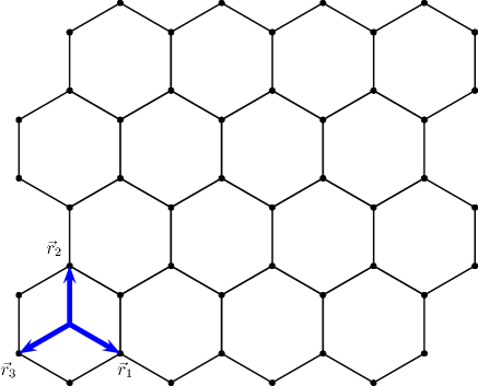
Figure 1: Representation of the graphene monolayer with the nearest-neighbour vectors $r_{\alpha}$ connecting the two sublattices $\Lambda_{A}$ and $\Lambda_{B}$.

A graphene monolayer is a honeycomb array of atoms of carbon as depicted in Fig. 1. In a monolayer the electrons can hop between nearest-neighbour carbon atoms through $\pi$-orbitals with energy $t$. The unit cell of the graphene monolayer is composed of two type of carbon atoms and we denote them by $A$ and $B$. The whole lattice is devided in to two sublattices, the $\Lambda_{A}$-type and the $\Lambda_{B}$-type. The Hamiltonian describing the graphene monolayer reads

$$H_{0} = -t\sum_{r\in\Lambda_{A}}\sum_{\alpha=1}^{3}a^{\dagger}_{r}b_{r+r_{\alpha}}+h.c.,$$ (1)

where $a$ and $b$ stand for the $\pi$-electron creation and anihilation fermionic operator on the atoms of type $A$ and $B$ respectively. The vector $r_{\alpha}$ connects the two sublattices $\Lambda_{A}$ and $\Lambda_{B}$ and is given by $r_{\alpha}=ae_{\alpha}$ with $a$ the lattice parameter and $e_{1}=(1,0)$, $e_{2}=(-1/2,\sqrt{3}/2)$ and $e_{3}=(-1/2,-\sqrt{3}/2)$ are unit vectors. In the following the lattice parameter $a$ will be set equal to one and plays the role of the unit of length.

The diagonalisation of the Hamiltonian (1) leads to the kinetic energy $\varepsilon_{k}=t|\sum_{\alpha=1}^{3}e^{ik.e_{\alpha}}|$, where $e_{\alpha}$’s are the nearest-neighbour vectors of the graphene monolayer. The kinetic energy vanishes at the two independent nodal points $K_{+(-)}$ which are chosen as $K_{+}=\left(0,\frac{4\pi}{3\sqrt{3}}\right)$ and $K_{-}=-K_{+}$ in the Brillouin zone. At low energy the bare Hamiltonian $H_{0}$ of the $\pi$-electron can be rewritten by considering the energetic contributions arround the nodal points and reads Semenoff

$$H_{0} = -\Bigg{\{}\sum_{r}v_{F}u_{a}^{\dagger}(r)(2\partial_{\bar{z}})u_{b}(r)$$

$$+\sum_{r}v_{F}v_{a}^{\dagger}(r)(-2\partial_{z})v_{b}(r)+h.c.\Bigg{\}},$$

where we made use of the notations in the complex plan $z=x+iy$ and $\partial_{z}=\frac{1}{2}\left(\partial_{x}-i\partial_{y}\right)$. The velocity $v_{F}=\frac{3}{2}ta/\hbar$ where we set $\hbar=a=1$ (the kinetic energy becomes $\varepsilon_{p}=\hbar v_{F}|p|$). The amplitude $u_{a}(b)$ and $v_{a}(b)$ are smooth functional operators and are connected to the creation and annihilation operator $a$ and $b$ through the Fourier components $u_{a}(p)=a_{p+K_{+}},u_{b}(p)=b_{p+K_{+}}$ and $v_{a}(p)=a_{p+K_{-}},v_{b}(p)=b_{p+K_{-}}$ where $p$ is the wave vector. The Hamiltonian $H_{0}$ describes the hopping of the $\pi$-electrons in an undistorted lattice.

A lattice distortion can be modeled by a variation of the hopping parameter $\delta t_{r,\alpha}$ which depends on the position in the lattice $\vec{r}$ and on the direction $e_{\alpha}$. The corresponding Hamiltonian for the graphene monolayer reads

$$H_{K}=-\sum_{r\in\Lambda_{A}}\sum_{\alpha=1}^{3}\delta t_{r,\alpha}a^{\dagger}_{r}b_{r+b_{\alpha}}+h.c.$$ (2)

In the following we consider the Kekule distortion for which the bonds between the carbon atoms are arranged similar to the benzene molecule Chamon . The lattice is then pictured by an alternation of long and short bonds between the carbon atoms of types $A$ and $B$ Viet . The Kekule distortion is modeled by the hopping parameter $\delta t_{r,\alpha}$ and reads $\delta t_{r,\alpha}=\frac{1}{3}\left(\Delta(r)e^{iK_{+}r_{\alpha}}e^{iG.r}+\bar{\Delta}(r)e^{iK_{-}r_{\alpha}}e^{-iG.r}\right)$, where $\Delta(r)$ stands for the amplitude of the Kekule distortion and $K_{+(-)}$ are the nodal points in the Brillouin zone. The vector $G=K_{+}-K_{-}$ connects the two independent Dirac cones located at the nodal points $K_{+(-)}$. Focusing on the low-energy contributions of the Kekule distortion around the nodal points the Hamiltonian $H_{K}$ is given by

$$H_{K}=-\sum_{r\in\Lambda_{A}}\left[\Delta(r)u_{a}^{\dagger}(r)v_{b}(r)+\bar{\Delta}(r)v_{a}^{\dagger}(r)u_{b}(r)\right]+h.c.$$

The Hamiltonian describing the $\pi$-electrons in the graphene single-layer with a Kekule distortion is then the sum of the bare and Kekule Hamiltonians $H=H_{0}+H_{K}$. Using the fermionic spinor $\psi^{\dagger}=\left[u_{b}(r)u_{a}(r)v_{a}(r)v_{b}(r)\right]^{\dagger}$ the Hamiltonian $H$ can be rewritten in the quantum electrodynamic framework and reads

$$H=\int d^{2}\vec{r}\bar{\psi}(r)\left[v_{F}\gamma_{k}\partial_{k}+\widetilde{\widetilde{\Delta}}(r)\right]\psi(r),$$

where the gamma matrices are defined by $\gamma_{0}=\tau_{3}\otimes\tau_{3}$, $\gamma_{1}=v_{F}\tau_{1}\otimes\tau_{3}$ and $\gamma_{2}=v_{F}\tau_{2}\otimes\tau_{3}$, $\tau_{\{0,1,2\}}$ are the Pauli matrices. The element $\widetilde{\widetilde{\Delta}}(r)$ is a $4\times 4$ matrices related to the Kekule distortion amplitude $\Delta(r)$ by the relation $\widetilde{\widetilde{\Delta}}(r)=\left(\begin{array}[]{cc}0&\Delta(r)\tau_{3}\\ -\bar{\Delta}(r)\tau_{3}&0\end{array}\right)$. The aim of the present work being to characterize the behaviour of the dynamical mass generation for graphene monolayer in presence of an homogeneous Kekule distortion we reduce our study to the case $\Delta(r)=\Delta_{0}$. Finally for a system at temperature $T=1/\beta$ the action of the graphene monolayer is given by

$$S_{el}=\int_{0}^{\beta}d\tau\int d^{2}\vec{r}\bar{\psi}(r,\tau)\left[\gamma^{\mu}\partial_{\mu}+\widetilde{\widetilde{\Delta}}_{0}\right]\psi(r,\tau).$$ (3)

The presence of the electromagnetic field surrounding the graphene monolayer is also to be considered. Indeed the graphene monolayer is embedded in an electromagnetic field which spans the whole 3D space. However the electrons are confined in the 2D space delimited by the carbon atoms. Hence the density of charge and current verify $\rho(x,y,z)=\delta(z)\rho_{2D}(x,y)$ and $\vec{J}(x,y,z)=\delta(z)\vec{J}_{2D}(x,y)$. The electromagnetic field vector $\vec{a}$ and scalar $\phi$ potentials are related to the Green functions of the laplacian $2\sqrt{-\vec{\nabla}^{2}}$ rather than $\vec{\nabla}^{2}$ for the three-dimensionnal electromagnetic field DoreyMavromatos ; GusyninPRD . To describe the electromagnetic field embedding the graphene monolayer it is convenient to use the following Euclidean $QED_{3}$ action

$$S_{e.m.}=-\int d^{3}x\frac{1}{2\sqrt{-\partial^{2}}}f^{\mu\nu}f_{\mu\nu},$$ (4)

where $f_{\mu\nu}=\partial_{\mu}a_{\nu}-\partial_{\nu}a_{\mu}$ is the electromagnetic field tensor derived from the three-dimensionnal vector potential $a_{\mu}$. The Fourier transform of action (4) leads to the bare photon propagator $\Delta_{\mu\nu}^{(0)}=\left(\delta_{\mu\nu}-q_{\mu}q_{\nu}\right)/(2|q|)$ in Euclidean space. For finite temperature the imaginary-time component $q_{0}$ of the (2+1)-dimensionnal wave-vector $q=(q_{0},q_{1},q_{2})$ is given by the bosonic Matsubara frequency $q_{0}=2\pi n/\beta$ ($n$ is an integer and takes its values in the range $]-\infty,\infty[$).

Finally the full quantum electrodynamic action describing the graphene monolayer with an homogeneous Kekule distortion and embedded in a 3D electromagnetic field reads $S=S_{e.m.}+S_{el}$

$$S = \int d^{3}x\frac{-1}{2\sqrt{-\partial^{2}}}f_{\mu\nu}f^{\mu\nu}$$ (5)

$$+\int d^{3}x\bar{\psi}\left[\gamma^{\mu}\left(\partial_{\mu}-iga_{\mu}\right)+\widetilde{\widetilde{\Delta}}_{0}\right]\psi.$$

It is known that 2D systems described by a quantum electrodynamic action like (5) experience a dynamical mass generation for the fermionic field $\psi$ in interaction with an $U(1)$ gauge field. Appelquist et al. Appelquist1 ; Appelquist2 showed that at zero temperature the originally massless fermions can acquire a dynamically generated mass when the number $N$ of fermion flavors is lower than the critical value $N_{c}=32/\pi^{2}$. Later Maris Maris confirmed the existence of a critical value $N_{c}\simeq 3.3$ below which the dynamical mass can be generated. Since we consider only spin-$1/2$ systems, $N=2$ and hence $N<N_{c}$. At finite temperature Dorey and Mavromatos DoreyMavromatos and Lee Lee-98 showed that the dynamically generated mass vanishes at a temperature $T$ larger than the critical one $T_{c}$. More recents works have been performed on dynamical mass generation in graphene monolayer Khveshchenko ; LealKhveshchenko . However the question now arise about the effects of a lattice distortion like the Kekule distortion. How does the mass generated dynamically in presence of a Kekule distortion behave? We concentrate on the effects of an homogeneous Kekule distortion and for small temperature $T\rightarrow 0$.

III Dynamical mass generation

III.1 The photon propagator at finite temperature

Integrating over the fermion fields $\psi$ leads to a pure gauge Lagrangian $\mathcal{L}_{a}=\frac{1}{2}a_{\mu}\Delta_{\mu\nu}^{-1}a_{\nu}$ where $\Delta_{\mu\nu}$ is the dressed photon propagator from which we shall extract an effective interaction potential between two fermion and derive the dynamical mass of the fermions.

The finite temperature photon propagator in Euclidean space verifies the Dyson equation Das ; JR3

$$\Delta_{\mu\nu}^{-1} = {\Delta_{\mu\nu}^{(0)}}^{-1}+\Pi_{\mu\nu},$$

where the bare photon propagator $\Delta_{\mu\nu}^{(0)}$ is derived from the action of the bare electromagnetic field (4) and the polarisation function is obtained from the integration over the fermionic field $\psi$ in the action (5).

For the computation of the dynamically generated mass it is enough to consider the static temporal dressed photon propagator component $\Delta_{00}(q^{0}=0,\vec{q})$ for which the bare photon propagator component reads ${\Delta_{00}^{(0)}(q^{0}=0,\vec{q})}=1/2|q|$. The detailed calculation of the static temporal component of the polarisation function $\Pi_{00}(q^{0}=0,\vec{q})$ is given in appendix A and reads

$$\Pi^{00}(q^{0}=0,\vec{q}) = \int_{0}^{1}dx\left(\frac{\alpha}{2\pi v_{F}^{2}\beta}\right)\Bigg{\{}\ln\left(2\cosh{(\pi\Theta_{q})}\right)$$ (6)

$$-\left(\frac{\beta|\Delta_{0}|}{2}\right)^{2}\frac{\tanh{(\pi\Theta_{q})}}{(\pi\Theta_{q})}\Bigg{\}},$$

where $\beta$ is the inverse temperature and $\Theta_{q}=\left(\frac{\beta}{2\pi}\right)\sqrt{x(1-x)v_{F}^{2}\vec{q}^{2}+|\Delta_{0}|^{2}}$. The coupling parameter $\alpha$ is related to the number of fermion flavor $N=2$ and to the electron charge $g$, $\alpha=4g^{2}N$.

For very small temperature $T\rightarrow 0$ the polarization function (6) becomes

$$\Pi^{00}(q^{0}=0,\vec{q}) = \left(\frac{\alpha}{8\pi v_{F}^{2}}\right)\Bigg{[}|\Delta_{0}|$$

$$+\frac{\left(v_{F}q\right)^{2}-4|\Delta_{0}|^{2}}{2v_{F}|q|}\arctan\left(\frac{v_{F}q}{2|\Delta_{0}|}\right)\Bigg{]}.$$

The process of dynamical mass generation is dominated by mechanisms at large wave vectors $\vec{q}$. Indeed for $q\gg 2|\Delta_{0}|/v_{F}$ the polarisation function is asymptoticaly equal to $\frac{\alpha}{16\pi v_{F}}|q|$ which confirms the fact that the dynamics between electrons and holes are dominated by large wave vectors Gusynin .

III.2 The electron self-energy

We now derives the electron self-energy which is also the dynamical mass. The Schwinger-Dyson equation for the electron propagator at finite temperature reads

$$G^{-1}(k) = {G^{(0)}}^{-1}(k)$$

$$- \frac{g}{\beta}\underset{\widetilde{\omega}_{F,n}}{\sum}\int\frac{d^{2}\vec{P}}{(2\pi)^{2}}\gamma_{\mu}G(p)\Delta_{\mu\nu}(k-p)\Gamma_{\nu},$$

where $p=(p_{0}=\widetilde{\omega}_{F,n},\vec{P})$, $G$ is the dressed electron propagator, $\Gamma_{\nu}$ the electron-photon vertex which will be approximated here by its bare value $g\gamma_{\nu}$ and $\Delta_{\mu\nu}$ is the dressed photon propagator. The second term in (LABEL:SchwingerDyson) is the fermion self-energy $\Sigma$, ($G^{-1}={G^{(0)}}^{-1}-\Sigma$). Performing the trace over the $\gamma$ matrices and working out the sum over the fermionic Matsubara frequencies $\widetilde{\omega}_{F,n}$ in equation (LABEL:SchwingerDyson) leads to a self-consistent equation for the self-energy of the form

$$\Sigma(\vec{k})=g^{2}\int\frac{d^{2}\vec{p}}{(2\pi)^{2}}\Delta_{00}(0,\vec{k}-\vec{p})\frac{\Sigma(\vec{p})}{2\varepsilon_{\vec{p}}}\tanh{\left(\frac{\beta\varepsilon_{\vec{p}}}{2}\right)},$$ (8)

where $\varepsilon_{\vec{p}}=\sqrt{\varepsilon^{(0)2}_{\vec{p}}+\Sigma(p)^{2}}$ and $\varepsilon^{(0)2}_{\vec{p}}=v_{F}^{2}\vec{p}^{2}+|\Delta_{0}|^{2}$ are respectively the energy spectrum of the graphene monolayer with and without correction of the one-loop approximation near the nodal points $K_{+(-)}$. In the limit $q\gg 2|\Delta_{0}|/v_{F}$ the dressed photon propagator is given by $\Delta_{00}(0,\vec{q})=\left[(2+\alpha/(16\pi v_{F}))|q|\right]^{-1}$. The angular integration in equation (8) is achieved using the approximation $f(|\vec{p}-\vec{k}|)=\theta(p-k)f(|p|)+\theta(k-p)f(|k|)$ where $f$ is a function which depends on the absolute value of its arguments Gusynin ; KhveshchenkoShively . Hence the self-consistent equation (8) reduces to

$$\Sigma(k) = C\Bigg{[}\int_{0}^{k}dp\frac{p\Sigma(p)}{k\sqrt{p^{2}+{(\widetilde{\Delta}(p)/v_{F})}^{2}}}$$ (9)

$$+\int_{k}^{\Lambda}dp\frac{\Sigma(p)}{\sqrt{p^{2}+{(\widetilde{\Delta}(p)/v_{F})}^{2}}}\Bigg{]},$$

where we introduced the constant $C=4g^{2}/\left(32\pi v_{F}+\alpha\right)$, the function $\widetilde{\Delta}(p)=\sqrt{|\Delta_{0}|^{2}+\Sigma(p)^{2}}$ and the ultraviolet cutoff $\Lambda$. The electron self-energy is assumed to be a small correction to the electron propagator. It follows that for $k\gg|\Delta_{0}|/v_{F}$ the denominator of the second term in equation (9) is approximately equal to $p$. In the first term of equation (9) the function $\widetilde{\Delta}(p)$ plays the role of a cutoff for $p\rightarrow 0$ and equation (9) can be rewritten $\Sigma(k)=C\left[\int_{\widetilde{\Delta}(p=0)/v_{F}}^{k}dp\frac{\Sigma(p)}{k}+\int_{k}^{\Lambda}dp\frac{\Sigma(p)}{p}\right]$. A derivation of this equation up to the second order with respect to the wave vector $k$ of the electron self-energy leads to the differential equation

$$k^{2}\Sigma^{{}^{\prime\prime}}(k)+2k\Sigma^{{}^{\prime}}(k)+C\Sigma(k)=0,$$ (10)

for which the infrared and ultraviolet boundary conditions are given respectively by

$$k^{2}\Sigma^{{}^{\prime}}(k){\Big{|}}_{k=\widetilde{\Delta}/v_{F}} = 0,\text{ and}$$ (11)

$$\left(k\Sigma^{{}^{\prime}}(k)+\Sigma(k)\right){\Big{|}}_{k=\Lambda} = 0.$$ (12)

The differential equation (10) admits a solution which verifies also the boundary conditions (11) and (12) and reads Appelquist2 ; Gusynin ; KhveshchenkoShively

$$\Sigma(k) = \frac{\widetilde{\Delta}^{3/2}}{\sin(\delta)\sqrt{v_{F}k}}\sin\left(\frac{\tan(\delta)}{2}\ln\left(\frac{v_{F}k}{\widetilde{\Delta}}\right)+\delta\right),$$

where the phase $\delta$ is equal to $\arctan\sqrt{4C-1}$. In order to verify the boundary condition (12) the amplitude $\widetilde{\Delta}(p=0)$ has to verify the following relation $\widetilde{\Delta}=(v_{F}\Lambda)\exp{\left[-4\delta/\sqrt{4C-1}\right]}$.

The solution of the electron self-energy has been derived for wave vectors larger than the cutoff $|\Delta_{0}|/v_{F}$ and shows to be independent of the amplitude $\Delta(r)=\Delta_{0}$ of the homogeneous Kekule distortion. The independence of $\Sigma$ on the amplitude $\Delta_{0}$ implies that the dynamical mass generation mechanism cannot be controlled by an homogeneous Kekule distortion.

It was shown elsewhere in the context of graphene bilayer that a gap opening in the energy spectrum can lead to an exciton instability under the specific amplitude of a short-ranged Coulomb interaction JHHanDR . Here a similar excitonic instability could appear since the graphene monolayer spectrum sees a gap open directly induced by the Kekule distortion. Moreover the gap is enlarged by formation of a mass which is dynamically generated. An exciton instability could take place KhveshchenkoShively . We address the question whether a Kekule distortion can amplify the mechanism of dynamical mass generation and consequently affect the exciton instability. The solution (LABEL:Eq13) for the electron self-energy $\Sigma$ shows that the dynamically generated mass of the electron is independent of the homogeneous Kekule distortion. However the mass of the electron given by $m(k)=\sqrt{|\Delta_{0}|^{2}+\Sigma(k)^{2}}=\langle\bar{\Psi}(k)\Psi(k)\rangle$ shows that the exciton instability resulting from the electron-hole interaction is directly dependent on the homogeneous Kekule distortion but not through the mechanism of dynamical mass generation.

IV Conclusions

The electron self-energy for graphene monolayer with an homogeneous Kekule distortion has been derived in the framework of quantum electrodynamics. It has been shown that the dynamical mass generation of the electrons resulting from the electron-hole interaction in the graphene monolayer is independent of the amplitude of the homogeneous Kekule distortion for a one-loop approximation. Such an independence of the dynamically generated mass provides an insight on the effects implied by lattice distortion on the energy spectrum of graphene monolayer.

The gap in the energy spectrum of the graphene monolayer is related to the mass of the electron which is equal to $m(k)=\sqrt{|\Delta_{0}|^{2}+\Sigma(k)^{2}}=\langle\bar{\Psi}(k)\Psi(k)\rangle$. The Kekule distortion control directly the gap by means of the amplitude $|\Delta_{0}|$ without any amplification through the dynamical mass $\Sigma$ (due to the independence mentioned previously). Consequently exciton instability can be formed by direct relation to the homogeneous Kekule distortion and by the Kekule-independent mechanism of dynamical mass generation.

So far we tried to shed light on the effects induced by lattice distortions such as an homogeneous Kekule distortion $\Delta(r)=\Delta_{0}$. The present study does not admit any conclusion on the independence of the dynamical mass $m(k)$ in presence of an inhomogeneous Kekule distortion $\Delta(r)\neq const$. It is expected that inhomogeneous lattice distortion affects significantly the energy spectrum of graphene monolayer. As a consequence exciton instability could possibly be amplified through lattice distortion via non-trivial dynamical mass generation.

Appendix A Derivation of the polarisation function

The polarisation function $\Pi_{\mu\nu}$ is obtained by integrating the $QED_{3}$ action (5) over the fermionic field $\psi$ and reads

$$\Pi^{\mu\nu}(q)=\frac{g^{2}}{\beta}\sum_{\sigma=\pm}\sum_{\omega_{f}}\int\frac{d^{2}\vec{k}}{(2\pi)^{2}}\text{Tr}\left[G_{0}(k).\gamma^{\mu}.G_{0}(k+q).\gamma^{\nu}\right]$$

where $G_{0}(k)=\frac{\gamma^{\rho}k_{\rho}+i\widetilde{\widetilde{\Delta}}_{0}}{k^{2}+|\Delta_{0}|^{2}}$ is the electron Green function and the trace operator Tr runs over the space of the gamma matrices. Focusing only on the static temporal component of the polarisation $\Pi_{00}(q^{0}=0,\vec{q})$ and using the following relations $\text{Tr}\left[i\widetilde{\widetilde{\Delta}}_{0}\gamma^{0}i\widetilde{\widetilde{\Delta}}_{0}\gamma^{0}\right]=-4|\Delta_{0}|^{2}$ and $\text{Tr}\left[\gamma^{\rho}k_{\rho}.\gamma^{0}\gamma^{\eta}(k_{\eta}+q_{\eta})\gamma^{0}\right]=4g^{(M)}_{\rho\eta}k_{\rho}(k_{\eta}+q_{\eta})$ where we defined the metric tensor $g^{(M)}_{\rho\eta}=diag(1,-v_{F}^{2},-v_{F}^{2})$, the polarisation function can be reduced to

$$\Pi^{00}(q)=\frac{g^{2}}{\beta}\sum_{\sigma=\pm}\sum_{\omega_{f}}\int\frac{d^{2}\vec{k}}{(2\pi)^{2}}\Bigg{(}\frac{1}{k^{2}+|\Delta_{0}|^{2}}$$

$$\times\frac{1}{(k+q)^{2}+|\Delta_{0}|^{2}}\Bigg{)}\times\Bigg{\{}4g^{(M)}_{\rho\eta}k_{\rho}(k_{\eta}+q_{\eta})-4|\Delta_{0}|^{2}\Bigg{\}}$$

(14)

The computation of the polarisation function can be simplified using the Feynmann identity $\frac{1}{ab}=\int_{0}^{1}dx\frac{1}{\left(ax+(1-x)b\right)^{2}}$, applying the change of variable $k\rightarrow k^{{}^{\prime}}-xq$ (in other words $\omega_{f}^{{}^{\prime}}=\frac{2\pi}{\beta}\left(n+1/2\right)$ and $\vec{k}^{{}^{\prime}}=\vec{k}+x\vec{q}$) and performing the sum over the fermionic Matsubara frequencies $\omega^{{}^{\prime}}_{f}$ one gets

$$\Pi^{00}(q^{0}=0,\vec{q})=$$

$$\frac{\alpha}{\beta}\int\frac{d^{2}\vec{k}^{{}^{\prime}}}{(2\pi)^{2}}\int_{0}^{1}dx\Bigg{\{}S_{1}-2\left(v_{F}^{2}\vec{k}^{{}^{\prime}2}+|\Delta_{0}|^{2}\right)S_{2}\Bigg{\}}$$

We define by $S_{1}$ and $S_{2}$ the sums over the Matsubara frequencies given by the following relations Gradshteyn

$$S_{1} \equiv \sum_{n=-\infty}^{\infty}\frac{1}{\left[{\omega^{{}^{\prime}}}^{2}+v_{F}^{2}\vec{k}^{{}^{\prime}2}+x(1-x)v_{F}^{2}\vec{q}^{2}+|\Delta_{0}|^{2}\right]}$$

$$= \frac{\beta^{2}}{4\pi Y}\tanh(\pi Y)$$

$$S_{2} \equiv \sum_{n=-\infty}^{\infty}\frac{1}{\left[{\omega^{{}^{\prime}}}^{2}+v_{F}^{2}\vec{k}^{{}^{\prime}2}+x(1-x)v_{F}^{2}\vec{q}^{2}+|\Delta_{0}|^{2}\right]}$$

$$= -\frac{\beta^{2}}{8\pi^{2}}\frac{1}{Y}\frac{\partial S_{1}}{\partial Y}$$

where $\omega^{{}^{\prime}}=\frac{2\pi}{\beta}(n+1/2)$. The integration over the wave vector $k^{{}^{\prime}}$ can be performed through the change of variable $Y=\frac{\beta}{2\pi}\sqrt{v_{F}^{2}\vec{k}^{{}^{\prime}2}+x(1-x)v_{F}^{2}\vec{q}^{2}+|\Delta_{0}|^{2}}$ and finally the polarisation function reads

$$\Pi^{00}(q^{0}=0,\vec{q}) = \frac{\alpha}{\beta}\int_{0}^{1}dx\lim_{\Lambda\rightarrow\infty}\int_{\Theta_{q}}^{\Lambda}\frac{2\pi}{(v_{F}\beta)^{2}}YdY\left[S_{1}+Y\frac{\partial S_{1}}{\partial Y}\right]$$

$$-\frac{\alpha}{\beta}\int_{0}^{1}dx\lim_{\Lambda\rightarrow\infty}\int_{\Theta_{q}}^{\Lambda}\frac{dY}{2\pi}x(1-x)\vec{q}^{2}\frac{\partial S_{1}}{\partial Y}$$

$$= \int_{0}^{1}dx\left(\frac{\alpha}{2\pi v_{F}^{2}\beta}\right)\Bigg{\{}\ln\left(2\cosh{(\pi\Theta_{q})}\right)$$

$$-\left(\frac{\beta|\Delta_{0}|}{2}\right)^{2}\frac{\tanh{(\pi\Theta_{q})}}{(\pi\Theta_{q})}\Bigg{\}}$$

where $\Theta_{q}=\left(\frac{\beta}{2\pi}\right)\sqrt{x(1-x)v_{F}^{2}\vec{q}^{2}+|\Delta_{0}|^{2}}$.

References

- (1) K. S. Novoselov, A. K. Geim, S. V. Morozov, D. Jiang, M. I. Katsnelson, I. V. Grigorieva, S. V. Dubonos, A. A. Firsov, Nature (London) 438,197 (2005).
- (2) K. S. Novoselov, E. McCann, S. V. Morozov, V. I. Falko, M. I. Katsnelson, U. Zeitler, D. Jiang, F. Schedin, A. K. Geim, Nature Physics 2, 177 (2006).
- (3) Y. Zhang, Y.-W. Tan, H. L. Stormer, and P. Kim, Nature (London) 438, 201 (2005).
- (4) A.K. Geim, and K.S. Novoselov, Nature Materials 6, 183 (2007).
- (5) E. McCann, V.I. Fal’ko, Phys. Rev. Lett. 96, 086805 (2006).
- (6) D.S.L. Abergel, Vladimir I. Fal’ko, Phys. Rev. B 75, 155430 (2007).
- (7) G. Baskaran, S.A. Jafari, Phys. Rev. Lett. 89, 016402 (2002).
- (8) N.M.R. Peres, F. Guinea, A.H. Castro Neto, Phys. Rev. B 73, 125411 (2006).
- (9) G. Semenoff, Phys. Rev. Lett. 53, 2449 (1984).
- (10) K.S. Novoselov, A.K. Geim, S.V. Morozov, D. Jiang, M.I. Katsnelson, I.V. Grigorieva, S.V. Dubonos, and A.A. Firsov, Nature 438, 197 (2005).
- (11) D.V.Khveshchenko, Phys. Rev. Lett. 87, 246802 (2001).
- (12) H. Leal, D.V.Khveshchenko, Nucl.Phys. B 687, 323 (2004).
- (13) D.V.Khveshchenko, W.F. Shively, Phys. Rev. B 73, 115104 (2006).
- (14) T.W. Appelquist, M. Bowick, D. Karabali and L.C.R. Wijewardhana, Phys. Rev. D 33, 3704 (1986).
- (15) E.V.Gorbar, V.P.Gusynin, V.A. Miransky, I.A. Shovkovy, Phys. Rev. B 66, 045108 (2002).
- (16) V.P. Gusynin, V.A. Miransky, I.A. Shovkovy, Phys. Rev. Lett. 73, 3499 (1994).
- (17) R. Dillenschneider, J.H. Han, arXiv:0709.1230 (2008). To be published in Phys. Rev. B.
- (18) E.V. Castro, K.S. Novoselov, S.V. Morozov, N.M.R. Peres, J.M.B. Lopes dos Santos, J. Nilsson, F. Guinea, A.K. Geim, and A.H. Castro Neto, Phys. Rev. Lett. 99, 216802 (2007).
- (19) J.B. Oostinga, H.B. Heersche, X. Liu, A.F. Morpurgo, and L.M.K. Vandersypen, Nature Materials 7, 151 (2007).
- (20) C. Chamon, C.-Y. Hou, R. Jackiw, C. Mudry, S.-Y. Pi, A.P.Schnyder, Phys. Rev. Lett. 100, 110405 (2008).
- (21) C.-Y. Hou, C. Chamon, C. Mudry, Phys. Rev. Lett. 98, 186809 (2007).
- (22) R. Jackiw, S.-Y. Pi, Phys. Rev. Lett. 98, 266402 (2007).
- (23) N. Dorey, N.E. Mavromatos, Nuclear Physics B 386, 614 (1992).
- (24) T.W. Appelquist, D. Nash and L.C.R. Wijewardhana, Phys. Rev. Lett. 60, 2575 (1988).
- (25) N.A. Viet, H. Ajiki, T. Ando, J. Phys. Soc. Jap. 63, 3036 (1994).
- (26) E.V. Gorbar, V.P. Gusynin, V.A. Miransky, Phys. Rev. D 64, 105028 (2001).
- (27) P. Maris, Phys. Rev. D 54, 4049 (1996).
- (28) D.J. Lee, Phys. Rev. D 58, 105012 (1998).
- (29) A. Das, Finite temperature field theory, World Scientific, (1997).
- (30) R. Dillenschneider, J. Richert, Phys. Rev. B 73, 224443 (2006).
- (31) I.S. Gradshteyn , I.M. Ryzhik, Table of Integrals, Series and Products. Academic Press, (1994).