New Mechanics of Spinal Injury

Abstract

The prediction and prevention of spinal injury is an important aspect of preventive health science. The spine, or vertebral column, represents a chain of 26 movable vertebral bodies, joint together by transversal viscoelastic intervertebral discs and longitudinal elastic tendons. This paper proposes a new locally–coupled loading–rate hypothesis, which states that the main cause of both soft– and hard–tissue spinal injury is a localized Euclidean jolt, or $SE(3)-$jolt, an impulsive loading that strikes a localized spine in several coupled degrees-of-freedom simultaneously. To show this, based on the previously defined covariant force law, we formulate the coupled Newton–Euler dynamics of the local spinal motions and derive from it the corresponding coupled $SE(3)-$jolt dynamics. The $SE(3)-$jolt is the main cause of two basic forms of spinal injury: (i) hard–tissue injury of local translational dislocations; and (ii) soft–tissue injury of local rotational disclinations. Both the spinal dislocations and disclinations, as caused by the $SE(3)-$jolt, are described using the Cosserat multipolar viscoelastic continuum model.

Keywords: localized spinal injury, coupled loading–rate hypothesis, coupled Newton–Euler
dynamics, Euclidean jolt dynamics, spinal dislocations and disclinations

Contact information:

Dr. Vladimir Ivancevic
Human Systems Integration, Land Operations Division
Defence Science & Technology Organisation, AUSTRALIA
PO Box 1500, 75 Labs, Edinburgh SA 5111
Tel:  +61 8 8259 7337,    Fax:  +61 8 8259 4193
E-mail:   Vladimir.Ivancevic$@$dsto.defence.gov.au

1 Introduction

Normal function of the human spine is possible due to a complex interaction of its components (i.e., vertebrae, ligaments, discs, rib cage, and muscles). Age, trauma, spinal disorders, and a host of other parameters can disrupt this interaction to an extent that in certain cases surgery may be required to restore normal function. Several spinal disorders have been described in [Goel et al 2006] from a mechanical perspective. An understanding of these disorders can assist in the design and development of spinal instrumentation. As biomechanics begins to be intertwined with tissue engineering, a better understanding of the particular disorders may also provide insight into ‘biological’ solutions.

In particular, the center of rotation of the upper cervical spine is an important biomechanical landmark that is used to determine upper neck moment, particularly when evaluating injury risk in the automotive environment [Chancey et al 2007]. Also, new vehicle safety standards are designed to limit the amount of neck tension and extension seen by out-of-position motor vehicle occupants during airbag deployments. The criteria used to assess airbag injury risk are currently based on volunteer data and animal studies due to a lack of bending tolerance data for the adult cervical spine [Nightingale et al 2007].

Also, lumbar spine pathology accounts for billions of dollars in societal costs each year. Although the symptomatology of these conditions is relatively well understood, the mechanical changes in the spine are not. Previous direct measurements of lumbar spine mechanics have mostly been performed on cadavers. The methods for in vivo studies have included imaging, electrogoniometry, and motion capture. Few studies have directly measured in vivo lumbar spine kinematics with in-dwelling bone pins. In vivo 3D motion of the entire lumbar spine has recently been tracked during gait in [Rozumalski et al 2008]. Using a direct (pin-based) in vivo measurement method, the motion of the human lumbar spine during gait was found to be triaxial. This appears to be the first 3D motion analysis of the entire lumbar spine using indwelling pins. The results were similar to previously published data derived from a variety of experimental methods.

The traditional principal loading hypothesis [McElhaney and Myers 1993, Whiting and Zernicke 1998], which describes general spinal injuries in terms of spinal tension, compression, bending, and shear, is insufficient to predict and prevent the cause of the back-pain syndrome. Its underlying mechanics is simply not accurate enough. On the other hand, to be recurrent, musculo-skeletal injury must be associated with a histological change, i.e., the modification of associated tissues within the body. However, incidences of functional musculoskeletal injury, e.g., lower back pain, generally shows little evidence of structural damage [Waddell 1998]. The incidence of injury is likely to be a continuum ranging from little or no evidence of structural damage through to the observable damage of muscles, joints or bones. The changes underlying functional injuries are likely to consist of torn muscle fibers, stretched ligaments, subtle erosion of join tissues, and/or the application of pressure to nerves, all amounting to a disruption of function to varying degrees and a tendency toward spasm.

For example, in a review of experimental studies on the role of mechanical stresses in the genesis of intervertebral disk degeneration and herniation [Rannou et al 2001], the authors dismissed simple mechanical stimulations of functional vertebra as a cause of disk herniation, concluding instead that a complex mechanical stimulation combining forward and lateral bending of the spine followed by violent compression is needed to produce posterior herniation of the disk. Considering the use of models to estimate the risk of injury the authors emphasize the need to understand this complex interaction between the mechanical forces and the living body [Seidel and Griffin 2001]. Compressive and shear loading increased significantly with exertion load, lifting velocity, and trunk asymmetry [Granata and Marras 1995]. Also, it has been stated that up to two–thirds of all back injuries have been associated with trunk rotation [Kumar and Narayan 2006]. In addition, load–lifting in awkward environment places a person at risk for low back pain and injury [Reiser et al 2008]. These risks appear to be increased when facing up or down an inclined surface.

The safe spinal motions (flexion/extension, lateral flexion and rotation) are governed by standard Euler’s rotational intervertebral dynamics coupled to Newton’s micro-translational dynamics. On the other hand, the unsafe spinal events, the main cause of spinal injuries, are caused by intervertebral SE(3)–jolts, the sharp and sudden, “delta”– (forces + torques) combined, localized both in time and in space. These localized intervertebral SE(3)–jolts do not belong to the standard Newton–Euler dynamics. The only way to monitor them would be to measure “in vivo” the rate of the combined (forces + torques)– rise.

It is well known that the mechanical properties of spinal ligaments and muscles are rate dependent. As elongation rate increases, ligaments generally exhibit higher stiffness, higher failure force, and smaller failure strain. Previous studies have shown that high-speed multiplanar loading causes soft tissue injury that is more severe as compared to sagittal loading. This paper proposes a new locally–coupled loading–rate hypothesis, which states that the main cause of both soft– and hard–tissue spinal injury is a localized Euclidean jolt, or $SE(3)-$jolt, an impulsive loading that strikes a localized spine in several coupled degrees-of-freedom (DOF) simultaneously. To show this, based on the previously defined covariant force law, we formulate the coupled Newton–Euler dynamics of the local spinal motions and derive from it the corresponding coupled $SE(3)-$jolt dynamics. The $SE(3)-$jolt is the main cause of two forms of local discontinuous spinal injury: (i) hard–tissue injury of local translational dislocations; and (ii) soft–tissue injury of local rotational disclinations. Both the spinal dislocations and disclinations, as caused by the $SE(3)-$jolt, are described using the Cosserat multipolar viscoelastic continuum model.

While we can intuitively visualize the SE(3)–jolt, for the purpose of simulation we use the necessary simplified, decoupled approach (neglecting the 3D torque matrix and its coupling to the 3D force vector). Note that decoupling is a kind of linearization that prevents chaotic behavior, giving an illusion of full predictability. In this decoupled framework of reduced complexity, we define:

The cause of hard spinal injuries (discus hernia) is a linear 3D–jolt vector hitting some intervertebral joint – the time rate-of-change of a 3D–force vector (linear jolt = mass $\times$ linear jerk).

The cause of soft spinal injuries (back–pain syndrome) is an angular 3–axial jolt hitting some intervertebral joint – the time rate-of-change of a 3–axial torque (angular jolt = inertia moment $\times$ angular jerk).

This decoupled framework has been implemented in the Human Biodynamics Engine [Ivancevic 2005], a world–class neuro–musculo–skeletal dynamics simulator (with 270 DOFs, the same number of equivalent muscular actuators and two–level neural reflex control), developed by the present author at Defence Science and Technology Organization, Australia. This kinematically validated human motion simulator has been described in a series of papers and books [Ivancevic and Snoswell 2001, Ivancevic and Beagley 2003, Ivancevic 2002, Ivancevic 2004, Ivancevic and Beagley 2005],
[Ivancevic and Ivancevic 2006a, Ivancevic and Ivancevic 2006b, Ivancevic and Ivancevic 2006c],
[Ivancevic and Ivancevic 2007e, Ivancevic 2006, Ivancevic and Ivancevic 2007a, Ivancevic and Ivancevic 2006, Ivancevic and Ivancevic 2007b, Ivancevic and Ivancevic 2008].

2 The $SE(3)-$jolt: the main cause of spinal injury

In the language of modern biodynamics [Ivancevic 2004, Ivancevic and Ivancevic 2006a],
[Ivancevic and Ivancevic 2006b, Ivancevic and Ivancevic 2006c, Ivancevic and Ivancevic 2007d],
[Ivancevic and Ivancevic 2007e], the general spinal motion is governed by the Euclidean SE(3)–group of 3D motions (see Figure 1). Within the spinal SE(3)–group we have both SE(3)–kinematics (consisting of the spinal SE(3)–velocity and its two time derivatives: SE(3)–acceleration and SE(3)–jerk) and the spinal SE(3)–dynamics (consisting of SE(3)–momentum and its two time derivatives: SE(3)–force and SE(3)–jolt), which is the spinal kinematics $\times$ the spinal mass–inertia distribution.

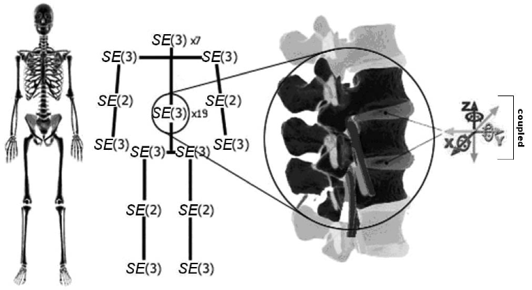
Figure 1: Human body representation in terms of SE(3)/SE(2)–groups of rigid–body motion, with the vertebral column represented as a chain of 26 flexibly–coupled SE(3)–groups.

Informally, the localized spinal SE(3)–jolt is a sharp and sudden change in the localized spinal SE(3)–force acting on the localized spinal mass–inertia distribution. That is, a ‘delta’–change in a 3D force–vector coupled to a 3D torque–vector, striking the certain local point along the vertebral column. In other words, the localized spinal SE(3)–jolt is a sudden, sharp and discontinues shock in all 6 coupled dimensions of a local spinal point, within the three Cartesian ($x,y,z$)–translations and the three corresponding Euler angles around the Cartesian axes: roll, pitch and yaw [Ivancevic and Beagley 2003]. If the SE(3)–jolt produces a mild shock to the spine, it causes mild, soft–tissue spinal injury, usually resulting in the back–pain sindrome. If the SE(3)–jolt produces a hard shock to the spine, it causes severe, hard–tissue spinal injury, with the total loss of movement.

Therefore, we propose a new combined loading–rate hypothesis of the local spinal injury instead of the old principal loading hypothesis. This new hypothesis has actually been supported by a number of individual studies, both experimental and numerical, as can be seen from the following brief review. One of the first dynamical studies of the head–neck system’s response to impulsive loading was performed in [Misra and Chakravarty 1985]. The response of a human head/neck/torso system to shock was investigated in [Luo and Goldsmith 1991], using a 3D numerical and physical models; the results indicated that the head, cervical muscles and disks in the lumbar region were subjected to the greatest force changes and thus were most likely to be injured. Time–dependent changes in the lumbar spine’s resistance to bending was investigated in [Adams and Dolan 1996], with the objective to show how time–related factors might affect the risk of back injury; the results suggested that the risk of bending injury to the lumbar discs and ligaments would depend not only on the loads applied to the spine, but also on loading rate. Cyclic loading tests were performed by [Tsai et al 1998] to investigate the mechanical responses at different loading rates; the results indicated that faster loading rate generated greater stress decay, and disc herniation was more likely to occur under higher loading rate conditions. Anterior shear of spinal motion segments was experimentally investigated in [Yingling and McGill 1999]; kinematics, kinetics, and resultant injuries were observed; dynamic loading and flexion of the specimens were found to increase the ultimate load at failure when compared with quasi-static loading and neutral postures. Experimental evidence concerning the distribution of forces and moments acting on the lumbar spine was reviewed in [Dolan and Adams 2001], pointing out that it was necessary to distribute the overall forces and moments between (and within) different spinal structures, because it was the concentration of force which caused injury, and elicited pain. Small magnitudes of axial torque was shown to in [Drake et al 2005] to alter the failure mechanics of the intervertebral disc and vertebrae in combined loading situations. A finite element model of head and cervical spine based on the actual geometry of a human cadaver specimen was developed in [Zhang et al 2006], which predicted the nonlinear moment-rotation relationship of human cervical spine. Vertebral end-plate fractures as a result of high–rate pressure loading were investigated in [Brown et al 2008], where a slightly exponential relationship was found between peak pressure and its rate of development.

The localized spinal SE(3)–jolt is rigorously defined in terms of differential geometry
[Ivancevic and Ivancevic 2006c, Ivancevic and Ivancevic 2007e]. Briefly, it is the absolute time–derivative of the covariant force 1–form (or, co-vector field) applied to the spine at a certain local point. With this respect, recall that the fundamental law of biomechanics – the so–called covariant force law [Ivancevic and Ivancevic 2006b, Ivancevic and Ivancevic 2006c, Ivancevic and Ivancevic 2007e], states:

$$\text{Force co-vector field}=\text{Mass distribution}\times\text{Acceleration vector--field},$$

which is formally written (using the Einstein summation convention, with indices labelling the three local Cartesian translations and the corresponding three local Euler angles):

$$F_{{\mu}}=m_{{\mu}{\nu}}a^{{\nu}},\qquad({\mu,\nu}=1,...,6=3\text{ Cartesian}+3\text{ Euler})$$

where $F_{{\mu}}$ denotes the 6 covariant components of the localized spinal SE(3)–force co-vector field, $m_{{\mu}{\nu}}$ represents the 6$\times$6 covariant components of the localized spinal inertia–metric tensor, while $a^{{\nu}}$ corresponds to the 6 contravariant components of localized spinal SE(3)–acceleration vector-field.

Now, the covariant (absolute, Bianchi) time–derivative $\frac{{D}}{dt}(\cdot)$ of the covariant SE(3)–force $F_{{\mu}}$ defines the corresponding localized spinal SE(3)–jolt co-vector field:

$$\frac{{D}}{dt}(F_{{\mu}})=m_{{\mu}{\nu}}\frac{{D}}{dt}(a^{{\nu}})=m_{{\mu}{\nu}}\left(\dot{a}^{{\nu}}+\Gamma_{\mu\lambda}^{{\nu}}a^{{\mu}}a^{{\lambda}}\right),$$ (1)

where ${\frac{{D}}{dt}}{(}a^{{\nu}})$ denotes the 6 contravariant components of the localized spinal SE(3)–jerk vector-field and overdot ($\dot{~{}}$) denotes the time derivative. $\Gamma_{\mu\lambda}^{{\nu}}$ are the Christoffel’s symbols of the Levi–Civita connection for the SE(3)–group, which are zero in case of pure Cartesian translations and nonzero in case of rotations as well as in the full–coupling of translations and rotations.

In the following, we elaborate on the localized spinal SE(3)–jolt concept (using vector and tensor methods) and its biophysical consequences in the form of the localized spinal dislocations and disclinations.

2.1 $SE(3)-$group of local spinal motions

Briefly, the $SE(3)-$group of localized spinal motions is defined as a semidirect (noncommutative) product of 3D intervertebral rotations and 3D intervertebral micro–translations,

$$SE(3):=SO(3)\rhd\mathbb{R}^{3}.$$

Its most important subgroups are the following (see Appendix for technical details):

In other words, the gauge $SE(3)-$group of intervertebral Euclidean micro-motions contains matrices of the form $\left(\begin{array}[]{cc}\mathbf{R}&\mathbf{p}\\ 0&1\end{array}\right),$ where $\mathbf{p}$ is intervertebral 3D micro-translation vector and $\mathbf{R}$ is intervertebral 3D rotation matrix, given by the product $\mathbf{R}=R_{\varphi}\cdot R_{\psi}\cdot R_{\theta}$ of the three Eulerian intervertebral rotations, $\text{roll}=R_{\varphi},~{}\text{pitch}=R_{\psi},~{}\text{yaw}=R_{\theta}$, performed respectively about the $x-$axis by an angle $\varphi,$ about the $y-$axis by an angle $\psi,$ and about the $z-$axis by an angle $\theta$ (see [Ivancevic 2004, Park and Chung 2005, Ivancevic 2006]),

$$R_{\varphi}=\left[\begin{array}[]{ccc}1&0&0\\ 0&\cos\varphi&-\sin\varphi\\ 0&\sin\varphi&\cos\varphi\end{array}\right],~{}~{}R_{\psi}=\left[\begin{array}[]{ccc}\cos\psi&0&\sin\psi\\ 0&1&0\\ -\sin\psi&0&\cos\psi\end{array}\right],~{}~{}R_{\theta}=\left[\begin{array}[]{ccc}\cos\theta&-\sin\theta&0\\ \sin\theta&\cos\theta&0\\ 0&0&1\end{array}\right].$$

Therefore, natural intervertebral $SE(3)-$dynamics is given by the coupling of Newtonian (translational) and Eulerian (rotational) equations of intervertebral motion.

2.2 Localized spinal $SE(3)-$dynamics

To support our locally–coupled loading–rate hypothesis, we formulate the coupled Newton–Euler dynamics of localized spinal motions within the $SE(3)-$group. The forced Newton–Euler equations read in vector (boldface) form

Newton $$: ~{}\mathbf{\dot{p}}~{}\mathbf{\equiv M\dot{v}=F+p\times\omega},$$ (2)

Euler $$: ~{}\mathbf{\dot{\pi}}~{}\mathbf{\equiv I\dot{\omega}=T+\pi\times\omega+p\times v},$$

where $\times$ denotes the vector cross product,

$$\mathbf{M}\equiv M_{ij}=diag\{m_{1},m_{2},m_{3}\}\qquad\text{and}\qquad\mathbf{I}\equiv I_{ij}=diag\{I_{1},I_{2},I_{3}\},\qquad(i,j=1,2,3)$$

are spinal segment’s (diagonal) mass and inertia matrices, defining the localized spinal mass–inertia distribution, with principal inertia moments given in Cartesian coordinates ($x,y,z$) by volume integrals

$$I_{1}=\iiint\rho(z^{2}+y^{2})dxdydz,~{}~{}I_{2}=\iiint\rho(x^{2}+z^{2})dxdydz,~{}~{}I_{3}=\iiint\rho(x^{2}+y^{2})dxdydz,$$

dependent on localized spinal density $\rho=\rho(x,y,z)$,

$$\mathbf{v}\equiv v^{i}=[v_{1},v_{2},v_{3}]^{t}\qquad\text{and\qquad}\mathbf{\omega}\equiv{\omega}^{i}=[\omega_{1},\omega_{2},\omega_{3}]^{t}$$

(where $[~{}]^{t}$ denotes the vector transpose) are localized spinal linear and angular velocity vectors (that is, column vectors),

$$\mathbf{F}\equiv F_{i}=[F_{1},F_{2},F_{3}]\qquad\text{and}\qquad\mathbf{T}\equiv T_{i}=[T_{1},T_{2},T_{3}]$$

are gravitational and other external force and torque co-vectors (that is, row vectors) acting on the spine,

$$\mathbf{p} \equiv p_{i}\equiv\mathbf{Mv}=[p_{1},p_{2},p_{3}]=[m_{1}v_{1},m_{2}v_{2},m_{2}v_{2}]\qquad\text{and}$$

$$\mathbf{\pi} \equiv \pi_{i}\equiv\mathbf{I\omega}=[\pi_{1},\pi_{2},\pi_{3}]=[I_{1}\omega_{1},I_{2}\omega_{2},I_{3}\omega_{3}]$$

are localized spinal linear and angular momentum co-vectors.

In tensor form, the forced Newton–Euler equations (2) read

$$\dot{p}_{i} \equiv M_{ij}\dot{v}^{j}=F_{i}+\varepsilon_{ik}^{j}p_{j}{\omega}^{k},\qquad(i,j,k=1,2,3)$$

$$\dot{\pi}_{i} \equiv I_{ij}\dot{\omega}^{j}=T_{i}+\varepsilon_{ik}^{j}\pi_{j}\omega^{k}+\varepsilon_{ik}^{j}p_{j}v^{k},$$

where the permutation symbol $\varepsilon_{ik}^{j}$ is defined as

$$\varepsilon_{ik}^{j}=\begin{cases}+1&\text{if }(i,j,k)\text{ is }(1,2,3),(3,1,2)\text{ or }(2,3,1),\\ -1&\text{if }(i,j,k)\text{ is }(3,2,1),(1,3,2)\text{ or }(2,1,3),\\ 0&\text{otherwise: }i=j\text{ or }j=k\text{ or }k=i.\end{cases}$$

In scalar form, the forced Newton–Euler equations (2) expand as

Newton $$: \left\{\begin{array}[]{c}\dot{p}_{{}_{1}}={F_{1}}-{m_{3}}{v_{3}}{\omega_{2}}+{m_{2}}{v_{2}}{\omega_{3}}\\ \dot{p}_{{}_{2}}={F_{2}}+{m_{3}}{v_{3}}{\omega_{1}}-{m_{1}}{v_{1}}{\omega_{3}}\\ \dot{p}_{{}_{3}}={F_{3}}-{m_{2}}{v_{2}}{\omega_{1}}+{m_{1}}{v_{1}}{\omega_{2}}\end{array}\right.,$$ (6)

Euler $$: \left\{\begin{array}[]{c}\dot{\pi}_{{}_{1}}={T_{1}}+({m_{2}}-{m_{3}}){v_{2}}{v_{3}}+({I_{2}}-{I_{3}}){\omega_{2}}{\omega_{3}}\\ \dot{\pi}_{{}_{2}}={T_{2}}+({m_{3}}-{m_{1}}){v_{1}}{v_{3}}+({I_{3}}-{I_{1}}){\omega_{1}}{\omega_{3}}\\ \dot{\pi}_{{}_{3}}={T_{3}}+({m_{1}}-{m_{2}}){v_{1}}{v_{2}}+({I_{1}}-{I_{2}}){\omega_{1}}{\omega_{2}}\end{array}\right.,$$ (10)

showing localized spinal mass and inertia couplings.

Equations (2)–(6) can be derived from the translational + rotational kinetic energy of the spine segment

$$E_{k}={\frac{1}{2}}\mathbf{v}^{t}\mathbf{Mv}+{\frac{1}{2}}\mathbf{\omega}^{t}\mathbf{I\omega},$$ (11)

or, in tensor form

$$E={\frac{1}{2}}M_{ij}{v}^{i}{v}^{j}+{\frac{1}{2}}I_{ij}{\omega}^{i}{\omega}^{j}.$$

For this we use the Kirchhoff–Lagrangian equations (see, e.g., [Lamb 1932, Leonard 1997], or the original work of Kirchhoff in German)

$$\frac{d}{{dt}}\partial_{\mathbf{v}}E_{k} = \partial_{\mathbf{v}}E_{k}\times\mathbf{\omega}+\mathbf{F},$$ (12)

$${\frac{d}{{dt}}}\partial_{\mathbf{\omega}}E_{k} = \partial_{\mathbf{\omega}}E_{k}\times\mathbf{\omega}+\partial_{\mathbf{v}}E_{k}\times\mathbf{v}+\mathbf{T},$$

where $\partial_{\mathbf{v}}E_{k}=\frac{\partial E_{k}}{\partial\mathbf{v}},~{}\partial_{\mathbf{\omega}}E_{k}=\frac{\partial E_{k}}{\partial\mathbf{\omega}}$; in tensor form these equations read

$$\frac{d}{dt}\partial_{v^{i}}E = \varepsilon_{ik}^{j}\left(\partial_{v^{j}}E\right)\omega^{k}+F_{i},$$

$$\frac{d}{dt}\partial_{{\omega}^{i}}E = \varepsilon_{ik}^{j}\left(\partial_{{\omega}^{j}}E\right){\omega}^{k}+\varepsilon_{ik}^{j}\left(\partial_{v^{j}}E\right)v^{k}+T_{i}.$$

Using (11)–(12), localized spinal linear and angular momentum co-vectors are defined as

$$\mathbf{p}=\partial_{\mathbf{v}}E_{k}{,\qquad\mathbf{\pi}=\partial_{\mathbf{\omega}}E_{k},}$$

or, in tensor form

$$p_{i}=\partial_{v^{i}}E{,\qquad}\pi_{i}=\partial_{{\omega}^{i}}E,$$

with their corresponding time derivatives, in vector form

$$~{}\mathbf{\dot{p}}=\frac{d}{dt}\mathbf{p=}\frac{d}{dt}\partial_{\mathbf{v}}E{,\qquad\mathbf{\dot{\pi}}=}\frac{d}{dt}\mathbf{\pi=}\frac{d}{dt}\partial_{\mathbf{\omega}}E,$$

or, in tensor form

$$~{}\dot{p}_{i}=\frac{d}{dt}p_{i}=\frac{d}{dt}\partial_{v^{i}}E{,\qquad\dot{\pi}_{i}=}\frac{d}{dt}\pi_{i}=\frac{d}{dt}\partial_{{\omega}^{i}}E,$$

or, in scalar form

$$\mathbf{\dot{p}}=[\dot{p}_{1},\dot{p}_{2},\dot{p}_{3}]=[m_{1}\dot{v}_{1},m_{2}\dot{v}_{2},m_{3}\dot{v}_{3}],\qquad{\mathbf{\dot{\pi}}}=[\dot{\pi}_{1},\dot{\pi}_{2},\dot{\pi}_{3}]=[I_{1}\dot{\omega}_{1},I_{2}\dot{\omega}_{2},I_{3}\dot{\omega}_{3}].$$

While spinal healthy $SE(3)-$dynamics is given by the coupled Newton–Euler micro–dynamics, the localized spinal injury is actually caused by the sharp and discontinuous change in this natural $SE(3)$ micro-dynamics, in the form of the $SE(3)-$jolt, causing localized discontinuous spinal deformations, both translational dislocations and rotational disclinations.

2.3 Localized spinal–injury dynamics: the $SE(3)-$jolt

The $SE(3)-$jolt, the actual cause of spinal injury (in the form of the localized spinal plastic deformations), is defined as a coupled Newton+Euler jolt; in (co)vector form the $SE(3)-$jolt reads

$$SE(3)-\text{jolt}:\left\{\begin{array}[]{l}\text{Newton~{}jolt}:\mathbf{\dot{F}=\ddot{p}-\dot{p}\times\omega-p\times\dot{\omega}}~{},\\ \text{Euler~{}jolt}:\mathbf{\dot{T}=\ddot{\pi}}~{}\mathbf{-\dot{\pi}\times\omega-\pi\times\dot{\omega}-\dot{p}\times v-p\times\dot{v}},\end{array}\right.$$

where the linear and angular jolt co-vectors are

$$\mathbf{\dot{F}\equiv M\ddot{v}}=[\dot{F}_{{1}},\dot{F}_{{2}},\dot{F}_{{3}}],\qquad\mathbf{\dot{T}\equiv I\ddot{\omega}}=[\dot{T}_{{1}},\dot{T}_{{2}},\dot{T}_{{3}}],$$

where

$$\mathbf{\ddot{v}}=[\ddot{v}_{{1}},\ddot{v}_{{2}},\ddot{v}_{{3}}]^{t},\qquad\mathbf{\ddot{\omega}}=[\ddot{\omega}_{{1}},\ddot{\omega}_{{2}},\ddot{\omega}_{{3}}]^{t},$$

are linear and angular jerk vectors.

In tensor form, the $SE(3)-$jolt reads

$$~{}\dot{F}_{i} = \ddot{p}_{i}-\varepsilon_{ik}^{j}\dot{p}_{j}{\omega}^{k}-\varepsilon_{ik}^{j}p_{j}{\dot{\omega}}^{k},\qquad(i,j,k=1,2,3)$$

$$~{}\dot{T}_{{i}} = \ddot{\pi}_{i}~{}-\varepsilon_{ik}^{j}\dot{\pi}_{j}\omega^{k}-\varepsilon_{ik}^{j}\pi_{j}{\dot{\omega}}^{k}-\varepsilon_{ik}^{j}\dot{p}_{j}v^{k}-\varepsilon_{ik}^{j}p_{j}\dot{v}^{k},$$

in which the linear and angular jolt covectors are defined as

$$\mathbf{\dot{F}} \equiv \dot{F}_{i}=\mathbf{M\ddot{v}}\,\equiv\mathbf{\,}M_{ij}\ddot{v}^{j}=[\dot{F}_{1},\dot{F}_{2},\dot{F}_{3}],$$

$$\mathbf{\dot{T}} \equiv \dot{T}_{{i}}=\mathbf{I\ddot{\omega}\equiv\,}I_{ij}\ddot{\omega}^{j}=[\dot{T}_{{1}},\dot{T}_{{2}},\dot{T}_{{3}}],$$

where  $\mathbf{\ddot{v}}=\ddot{v}^{{i}},$ and $\mathbf{\ddot{\omega}}=\ddot{\omega}^{{i}}$ are linear and angular jerk vectors.

In scalar form, the $SE(3)-$jolt expands as

Newton jolt $$: \left\{\begin{array}[]{l}\dot{F}_{{1}}=\ddot{p}_{1}-m_{{2}}\omega_{{3}}\dot{v}_{{2}}+m_{{3}}\left({\omega}_{{2}}\dot{v}_{{3}}+v_{{3}}\dot{\omega}_{{2}}\right)-m_{{2}}v_{{2}}{\dot{\omega}}_{{3}},\\ \dot{F}_{{2}}=\ddot{p}_{2}+m_{{1}}\omega_{{3}}\dot{v}_{{1}}-m_{{3}}\omega_{{1}}\dot{v}_{{3}}-m_{{3}}v_{{3}}\dot{\omega}_{{1}}+m_{{1}}v_{{1}}\dot{\omega}_{{3}},\\ \dot{F}_{{3}}=\ddot{p}_{3}-m_{{1}}\omega_{{2}}\dot{v}_{{1}}+m_{{2}}\omega_{{1}}\dot{v}_{{2}}-v_{{2}}\dot{\omega}_{{1}}-m_{{1}}v_{{1}}\dot{\omega}_{{2}},\end{array}\right.$$

Euler jolt $$: \left\{\begin{array}[]{l}\dot{T}_{{1}}=\ddot{\pi}_{1}-(m_{{2}}-m_{{3}})\left(v_{{3}}\dot{v}_{{2}}+v_{{2}}\dot{v}_{{3}}\right)-(I_{{2}}-I_{{3}})\left(\omega_{{3}}\dot{\omega}_{{2}}+{\omega}_{{2}}{\dot{\omega}}_{{3}}\right),\\ \dot{T}_{{2}}=\ddot{\pi}_{2}+(m_{{1}}-m_{{3}})\left(v_{{3}}\dot{v}_{{1}}+v_{{1}}\dot{v}_{{3}}\right)+(I_{{1}}-I_{{3}})\left({\omega}_{{3}}{\dot{\omega}}_{{1}}+{\omega}_{{1}}{\dot{\omega}}_{{3}}\right),\\ \dot{T}_{{3}}=\ddot{\pi}_{3}-(m_{{1}}-m_{{2}})\left(v_{{2}}\dot{v}_{{1}}+v_{{1}}\dot{v}_{{2}}\right)-(I_{{1}}-I_{{2}})\left({\omega}_{{2}}{\dot{\omega}}_{{1}}+{\omega}_{{1}}{\dot{\omega}}_{{2}}\right).\end{array}\right.$$

We remark here that the linear and angular momenta ($\mathbf{p,\pi}$), forces ($\mathbf{F,T}$) and jolts ($\mathbf{\dot{F},\dot{T}}$) are co-vectors (row vectors), while the linear and angular velocities ($\mathbf{v,\omega}$), accelerations ($\mathbf{\dot{v},\dot{\omega}}$) and jerks ($\mathbf{\ddot{v},\ddot{\omega}}$) are vectors (column vectors). This bio-physically means that the ‘jerk’ vector should not be confused with the ‘jolt’ co-vector. For example, the ‘jerk’ means shaking the head’s own mass–inertia matrices (mainly in the atlanto–occipital and atlanto–axial joints), while the ‘jolt’means actually hitting the head with some external mass–inertia matrices included in the ‘hitting’ SE(3)–jolt, or hitting some external static/massive body with the head (e.g., the ground – gravitational effect, or the wall – inertial effect). Consequently, the mass-less ‘jerk’ vector represents a (translational+rotational) non-collision effect that can cause only soft–tissue spinal injuries, while the inertial ‘jolt’ co-vector represents a (translational+rotational) collision effect that can cause hard–tissue spinal injuries.

For example, while driving a car, the SE(3)–jerk of the head–neck system happens every time the driver brakes abruptly. On the other hand, the SE(3)–jolt means actual impact to the head. Similarly, the whiplash–jerk, caused by rear–end car collisions, is like a soft version of the high pitch–jolt caused by the boxing ‘upper-cut’. Also, violently shaking the head left–right in the transverse plane is like a soft version of the high yaw–jolt caused by the boxing ‘cross-cut’.

2.4 Localized spinal dislocations and disclinations caused by the $SE(3)-$jolt

Recall from introduction that for mild (soft–tissue) spinal injury, the best injury predictor is considered to be the product of localized spinal strain and strain rate, which is the standard isotropic viscoelastic continuum concept. To improve this standard concept, in this subsection, we consider spinal segment (with a vertebral body, intervertebral disc and other visco-elastic tissue) as a 3D anisotropic multipolar Cosserat viscoelastic continuum [Cosserat and Cosserat 1898, Cosserat and Cosserat 1909, Eringen 2002], exhibiting coupled–stress–strain elastic properties. This non-standard continuum model is suitable for analyzing plastic (irreversible) deformations and fracture mechanics [Bilby and Eshelby 1968] in multi-layered materials with microstructure (in which slips and bending of layers introduces additional degrees of freedom, non-existent in the standard continuum models; see [Mindlin 1965, Lakes 1985] for physical characteristics and [Yang and Lakes 1981, Yang and Lakes 1982],
[Park and Lakes 1986] for biomechanical applications).

The $SE(3)-$jolt $(\mathbf{\dot{F},\dot{T}})$ causes two types of localized spinal discontinuous deformations:

1. The Newton jolt $\mathbf{\dot{F}}$ can cause micro-translational dislocations, or discontinuities in the Cosserat translations;

2. The Euler jolt $\mathbf{\dot{T}}$ can cause micro-rotational disclinations, or discontinuities in the Cosserat rotations.

For general treatment on dislocations and disclinations related to asymmetric discontinuous deformations in multipolar materials, see, e.g., [Jian and Xiao-ling 1995, Yang et al 2001].

To precisely define localized spinal dislocations and disclinations, caused by the $SE(3)-$jolt $(\mathbf{\dot{F},\dot{T}})$, we first define the coordinate co-frame, i.e., the set of basis 1–forms $\{dx^{i}\}$, given in local coordinates $x^{i}=(x^{1},x^{2},x^{3})=(x,y,z)$, attached to spinal segment’s center-of-mass. Then, in the coordinate co-frame $\{dx^{i}\}$ we introduce the following set of spinal segment’s plastic–deformation–related $SE(3)-$based differential $p-$forms (see [Ivancevic and Ivancevic 2006c, Ivancevic and Ivancevic 2007e]):
    the dislocation current 1–form, $\mathbf{J}=J_{i}\,dx^{i};$
    the dislocation density 2–form, $\mathbf{\alpha}=\frac{1}{2}\alpha_{ij}\,dx^{i}\wedge dx^{j};$
    the disclination current 2–form, $\mathbf{S}=\frac{1}{2}S_{ij}\,dx^{i}\wedge dx^{j};$  and
    the disclination density 3–form, $\mathbf{Q}=\frac{1}{3!}Q_{ijk}\,dx^{i}\wedge dx^{j}\wedge dx^{k}$,

where $\wedge$ denotes the exterior wedge–product. According to Edelen [Edelen 1980, Kadic and Edelen 1983], these four $SE(3)-$based differential forms satisfy the following set of continuity equations:

$$\mathbf{\dot{\alpha}}=\mathbf{-dJ-S,}$$ (15)

$$\mathbf{\dot{Q}}=\mathbf{-dS,}$$ (16)

$$\mathbf{d\alpha}=\mathbf{Q,}$$ (17)

$$\mathbf{dQ}=\mathbf{0,}\qquad$$ (18)

where $\mathbf{d}$ denotes the exterior derivative.

In components, the simplest, fourth equation (18), representing the Bianchi identity, can be rewritten as

$$\mathbf{dQ}=\partial_{l}Q_{[ijk]}\,dx^{l}\wedge dx^{i}\wedge dx^{j}\wedge dx^{k}=0,$$

where $\partial_{i}\equiv\partial/\partial x^{i}$, while $\theta_{[ij...]}$ denotes the skew-symmetric part of $\theta_{ij...}$.

Similarly, the third equation (17) in components reads

$$\frac{1}{3!}Q_{ijk}\,dx^{i}\wedge dx^{j}\wedge dx^{k} = \partial_{k}\alpha_{[ij]}\,dx^{k}\wedge dx^{i}\wedge dx^{j},\text{\qquad or}$$

$$Q_{ijk} = -6\partial_{k}\alpha_{[ij]}.$$

The second equation (16) in components reads

$$\frac{1}{3!}\dot{Q}_{ijk}\,dx^{i}\wedge dx^{j}\wedge dx^{k} = -\partial_{k}S_{[ij]}\,dx^{k}\wedge dx^{i}\wedge dx^{j},\text{\qquad or}$$

$$\dot{Q}_{ijk} = 6\partial_{k}S_{[ij]}.$$

Finally, the first equation (15) in components reads

$$\frac{1}{2}\dot{\alpha}_{ij}\,dx^{i}\wedge dx^{j} = (\partial_{j}J_{i}-\frac{1}{2}S_{ij})\,dx^{i}\wedge dx^{j},\text{\qquad or}$$

$$\dot{\alpha}_{ij}\, = 2\partial_{j}J_{i}-S_{ij}\,.$$

In words, we have:

• The 2–form equation (15) defines the time derivative $\mathbf{\dot{\alpha}=}\frac{1}{2}\dot{\alpha}_{ij}\,dx^{i}\wedge dx^{j}$ of the dislocation density $\mathbf{\alpha}$ as the (negative) sum of the disclination current $\mathbf{S}$ and the curl of the dislocation current $\mathbf{J}$.

• The 3–form equation (16) states that the time derivative $\mathbf{\dot{Q}=}\frac{1}{3!}\dot{Q}_{ijk}\,dx^{i}\wedge dx^{j}\wedge dx^{k}$ of the disclination density $\mathbf{Q}$ is the (negative) divergence of the disclination current $\mathbf{S}$.

• The 3–form equation (17) defines the disclination density $\mathbf{Q}$ as the divergence of the dislocation density $\mathbf{\alpha}$, that is, $\mathbf{Q}$ is the exact 3–form.

• The Bianchi identity (18) follows from equation (17) by Poincaré lemma [Ivancevic and Ivancevic 2006c, Ivancevic and Ivancevic 2007e] and states that the disclination density $\mathbf{Q}$ is conserved quantity, that is, $\mathbf{Q}$ is the closed 3–form. Also, every 4–form in 3D space is zero.

From these equations, we can conclude that localized spinal dislocations and disclinations are mutually coupled by the underlaying $SE(3)-$group, which means that we cannot separately analyze translational and rotational spinal injuries — a fact which is not supported by the literature.

3 Conclusion

Based on the previously developed covariant force law, in this paper we have formulated a new coupled loading–rate hypothesis, which states that the main cause of localized spinal injury is an external $SE(3)-$jolt, an impulsive loading striking the spinal segment in several degrees-of-freedom, both rotational and translational, combined. To demonstrate this, we have developed the vector Newton–Euler mechanics on the Euclidean $SE(3)-$group of localized spinal micro-motions. In this way, we have precisely defined the concept of the $SE(3)-$jolt, which is a cause of rapid localized spinal discontinuous deformations: (i) mild rotational disclinations and (ii) severe translational dislocations. Based on the presented model, we argue that we cannot separately analyze localized spinal rotations from translations, as they are in reality coupled. To prevent spinal injuries we need to develop the internal SE(3)–jolt awareness. To maintain a healthy spine, we need to prevent localized SE(3)–jolts from striking any part of the spine in any human–motion or car–crash conditions.

4 Appendix: The $SE(3)-$group

Special Euclidean group $SE(3):=SO(3)\rhd\mathbb{R}^{3}$, (the semidirect product of the group of rotations with the corresponding group of translations), is the Lie group consisting of isometries of the Euclidean 3D space $\mathbb{R}^{3}$.

An element of $SE(3)$ is a pair $(A,a)$ where $A\in SO(3)$ and $a\in\mathbb{R}^{3}.$ The action of $SE(3)$ on $\mathbb{R}^{3}$ is the rotation $A$ followed by translation by the vector $a$ and has the expression

$$(A,a)\cdot x=Ax+a.$$

The Lie algebra of the Euclidean group $SE(3)$ is $\mathfrak{se}(3)=\mathbb{R}^{3}\times\mathbb{R}^{3}$ with the Lie bracket

$$[(\xi,u),(\eta,v)]=(\xi\times\eta,\xi\times v-\eta\times u).$$ (19)

Using homogeneous coordinates, we can represent $SE(3)$ as follows,

$$SE(3)=\ \ \left\{\left(\begin{array}[]{cc}R&p\\ 0&1\end{array}\right)\in GL(4,\mathbb{R}):R\in SO(3),\,p\in\mathbb{R}^{3}\right\},$$

with the action on $\mathbb{R}^{3}$ given by the usual matrix–vector product when we identify $\mathbb{R}^{3}$ with the section $\mathbb{R}^{3}\times\{1\}\subset\mathbb{R}^{4}$. In particular, given

$$g=\left(\begin{array}[]{cc}R&p\\ 0&1\end{array}\right)\in SE(3),$$

and $q\in\mathbb{R}^{3}$, we have

$$g\cdot q=Rq+p,$$

or as a matrix–vector product,

$$\left(\begin{array}[]{cc}R&p\\ 0&1\end{array}\right)\left(\begin{array}[]{c}q\\ 1\end{array}\right)=\left(\begin{array}[]{c}Rq+p\\ 1\end{array}\right).$$

The Lie algebra of $SE(3)$, denoted $\mathfrak{se}(3)$, is given by

$$\mathfrak{se}(3)=\ \ \left\{\left(\begin{array}[]{cc}\omega&v\\ 0&0\end{array}\right)\in M_{4}(\mathbb{R}):\omega\in\mathfrak{so}(3),\,v\in\mathbb{R}^{3}\right\},$$

where the attitude (or, angular velocity) matrix $\omega:\mathbb{R}^{3}\rightarrow\mathfrak{so}(3)$ is given by

$$\omega=\left(\begin{array}[]{ccc}0&-\omega_{z}&\omega_{y}\\ \omega_{z}&0&-\omega_{x}\\ -\omega_{y}&\omega_{x}&0\end{array}\right).$$

The exponential map, $\exp:\mathfrak{se}(3)\rightarrow SE(3)$, is given by

$$\exp\left(\begin{array}[]{cc}\omega&v\\ 0&0\end{array}\right)=\left(\begin{array}[]{cc}\exp(\omega)&Av\\ 0&1\end{array}\right),$$

where

$$A=I+\frac{1-\cos\left\|\omega\right\|}{\left\|\omega\right\|^{2}}\omega+\frac{\left\|\omega\right\|-\sin\left\|\omega\right\|}{\left\|\omega\right\|^{3}}\omega^{2},$$

and $\exp(\omega)$ is given by the Rodriguez’ formula,

$$\exp(\omega)=I+\frac{\sin\left\|\omega\right\|}{\left\|\omega\right\|}\omega+\frac{1-\cos\left\|\omega\right\|}{\left\|\omega\right\|^{2}}\omega^{2}.$$

References

- [Goel et al 2006] Goel, V.K., Sairyoa, K., Vishnubhotl, S.L., Biyania, A., Ebraheim, N., Spine Technology Handbook, Chapter 6 - Spine Disorders: Implications for Bioengineers, Elsevier, (2006).
- [Chancey et al 2007] Chanceya, V.C., Ottavianoa, D., Myersa, B.S., Nightingale, R.W., J. Biomech., 40(9), 1953-1959, (2007).
- [Nightingale et al 2007] Nightingale, R.W., Chanceya, V.C., Ottaviano, D., Luck, J.F., Tran, L., Prange, M., Myersa, B.S., Flexion and extension structural properties and strengths for male cervical spine segments, J. Biomech., 40(3), 535-542, (2007).
- [Rozumalski et al 2008] Rozumalski, A., Schwartz, M.H., Wervey, R., Swanson, A., Dykes, D.C., Novacheck, T., The in vivo three-dimensional motion of the human lumbar spine during gait, Gait Posture, 18585041 (P,S,E,B,D), (2008)
- [McElhaney and Myers 1993] McElhaney, J.H., Myers, B.S. Biomechanical Aspects of Cervical Trauma, in: A.M. Nahum and J.W. Melvin (Eds.), Accidental injury: Biomechanics and Prevention, Springer, New York, (1993).
- [Whiting and Zernicke 1998] Whiting, W.C., Zernicke, R.F. Biomechanics of Musculoskeletal Injury. Human Kinetics, Champaign, IL, (1998).
- [Waddell 1998] Waddell, G. The Back Pain Revolution. Churchill Livingstone, Edinburgh, (1998).
- [Rannou et al 2001] Rannou, F., Corvol, M., Revel, M., Poiraudeau, S. Disk degeneration and disk herniation: the contribution of mechanical stress. Joint, Bone, Spine: Revue du Rheumatisme, 68(6), 543-546, (2001).
- [Seidel and Griffin 2001] Seidel, H., Griffin, M.J. Modelling the response of the spinal system to whole-body vibration and repeated shock. Clin. Biomech. 16(1), S3-7, (2001).
- [Granata and Marras 1995] Granata, K.P., Marras, W.S. An EMG-assisted model of trunk loading during free-dynamic lifting. J. Biomech. 28(11), 1309-17, (1995).
- [Kumar and Narayan 2006] Kumar, S., Narayan, Y., Torque and EMG in rotation extension of the torso from pre-rotated and flexed postures. Clin. Biomech. 21(9), 920–931, (2006).
- [Reiser et al 2008] Reiser, R.F., Wickel, E.E., Menzer, H.H., Lumbar mechanics of floor to knuckle height lifting on sloped surfaces. Int. J. Ind. Erg. 38(1), 47-55, (2008).
- [Ivancevic and Snoswell 2001] Ivancevic, V., Snoswell, M. Fuzzy-Stochastic Functor Machine for General Humanoid-Robot Dynamics. IEEE Trans. Sys. Man Cyber. B, 31(3), 319-330, (2001).
- [Ivancevic 2002] Ivancevic, V. Generalized Hamiltonian Biodynamics and Topology Invariants of Humanoid Robots. Int. J. Math. & Math. Sci. 31(9), 555-565, (2002).
- [Ivancevic 2004] Ivancevic, V. Symplectic Rotational Geometry in Human Biomechanics. SIAM Rev. 46(3), 455–474, (2004).
- [Ivancevic 2005] Ivancevic, V. Human Biodynamics Engine – Full Spine Simulator. Australian Defence Excellence in Science & Technology Award 2005 for Physiological Modelling, Adelaide, (2005).
- [Ivancevic and Beagley 2005] Ivancevic, V., Beagley, N. Brain-like functor control machine for general humanoid biodynamics. Int. J. Math. & Math. Sci. 11, 1759-1779, (2005).
- [Ivancevic 2006] Ivancevic, V., Lie-Lagrangian model for realistic human bio-dynamics. Int. J. Hum. Rob. 3(2), 205-218, (2006).