Compressed Sensing of Analog Signals in Shift-Invariant Spaces

Abstract

A traditional assumption underlying most data converters is that the signal should be sampled at a rate exceeding twice the highest frequency. This statement is based on a worst-case scenario in which the signal occupies the entire available bandwidth. In practice, many signals are sparse so that only part of the bandwidth is used. In this paper, we develop methods for low-rate sampling of continuous-time sparse signals in shift-invariant (SI) spaces, generated by m kernels with period T. We model sparsity by treating the case in which only k out of the m generators are active, however, we do not know which k are chosen. We show how to sample such signals at a rate much lower than m/T, which is the minimal sampling rate without exploiting sparsity. Our approach combines ideas from analog sampling in a subspace with a recently developed block diagram that converts an infinite set of sparse equations to a finite counterpart. Using these two components we formulate our problem within the framework of finite compressed sensing (CS) and then rely on algorithms developed in that context. The distinguishing feature of our results is that in contrast to standard CS, which treats finite-length vectors, we consider sampling of analog signals for which no underlying finite-dimensional model exists. The proposed framework allows to extend much of the recent literature on CS to the analog domain.

I Introduction

Digital applications have developed rapidly over the last few decades. Signal processing in the discrete domain inherently relies on sampling a continuous-time signal to obtain a discrete-time representation. The traditional assumption underlying most analog-to-digital converters is that the samples must be acquired at the Shannon-Nyquist rate, corresponding to twice the highest frequency [1, 2].

Although the bandlimited assumption is often approximately met, many signals can be more adequately modeled in alternative bases other than the Fourier basis [3, 4], or possess further structure in the Fourier domain. Research in sampling theory over the past two decades has substantially enlarged the class of sampling problems that can be treated efficiently and reliably. This resulted in many new sampling theories which accommodate more general signal sets as well as various linear and nonlinear distortions [5, 6, 4, 7, 8, 9, 10, 11].

A signal class that plays an important role in sampling theory are signals in shift-invariant (SI) spaces. Such functions can be expressed as linear combinations of shifts of a set of generators with period $T$ [12, 13, 14, 15, 16]. This model encompasses many signals used in communication and signal processing. For example, the set of bandlimited functions is SI with a single generator. Other examples include splines [4, 17] and pulse amplitude modulation in communications. Using multiple generators, a larger set of signals can be described such as multiband functions [18, 19, 20, 21, 22, 23]. Sampling theories similar to the Shannon theorem can be developed for this signal class, which allows to sample and reconstruct such functions using a broad variety of filters.

Any signal $x(t)$ in a SI space generated by $m$ functions shifted with period $T$ can be perfectly recovered from $m$ sampling sequences, obtained by filtering $x(t)$ with a bank of $m$ filters and uniformly sampling their outputs at times $nT$. The overall sampling rate of such a system is $m/T$. In Section II we show explicitly how to recover $x(t)$ from these samples by an appropriate filter bank. If the signal is generated by $k$ out of the $m$ generators, then as long as the chosen subset is known, it suffices to sample at a rate of $k/T$ corresponding to uniform samples with period $T$ at the output of $k$ filters. However, a more difficult question is whether the rate can be reduced if we know that only $k$ of the generators are active, but we do not know in advance which ones. Since in principle $x(t)$ may be comprised of any of the generators, it may seem at first that the rate cannot be lower than $m/T$.

This question is a special case of sampling a signal in a union of subspaces [24, 25, 26]. In our problem, $x(t)$ lies in one of the subspaces expressed by $k$ generators, however we do not know which subspace is chosen. Necessary and sufficient conditions where derived in [24, 25] to ensure that a sampling operator over such a union is invertible. In our setting this reduces to the requirement that the sampling rate is at least $2k/T$. However, no concrete sampling methods where given that ensure efficient and stable recovery, and no recovery algorithm was provided from a given set of samples. Finite-dimensional unions where treated in [26], for which stable recovery methods where developed. Another special case of sampling on a union of spaces that has been studied extensively is the problem underlying the field of compressed sensing (CS). In this setting, the goal is to recover a length $m$ vector ${{\bf x}}$ from $p<m$ linear measurements, where ${{\bf x}}$ is known to be $k$-sparse in some basis [27, 28]. Many stable and efficient recovery algorithms have been proposed to recover ${{\bf x}}$ in this setting [29, 30, 31, 32, 28, 33, 26].

A fundamental difference between our problem and mainstream CS papers is that we aim to sample and reconstruct continuous signals, while CS focuses on recovery of finite vectors. The methods developed in the context of CS rely on the finite nature of the problem and cannot be immediately adopted to infinite-dimensional settings without discretization or heuristics. Our goal is to directly reduce the analog sampling rate, without first requiring the Nyquist-rate samples and then applying finite-dimensional CS techniques.

Several attempts to extend CS ideas to the analog domain were developed in a set of conferences papers [34, 35]. However, in both papers an underlying discrete model was assumed which enabled immediate application of known CS techniques. An alternative analog framework is the work on finite rate of innovation [36, 37], in which $x(t)$ is modeled as a finite linear combination of shifted diracs (some extensions are given to other generators as well). The algorithms developed in this context exploit the similarity between the given problem and spectral estimation, and again rely on finite dimensional methods.

In contrast, the model we treat in this paper is inherently infinite dimensional as it involves an infinite sequence of samples from which we would like to recover an analog signal with infinitely many parameters. In such a setting the measurement matrix in standard CS is replaced by a more general linear operator. It is therefore no longer clear how to choose such an operator to ensure stability. Furthermore, even if a stable operator can be implemented, it will result in infinitely many compressed samples. As standard CS algorithms operate on finite-dimensional optimization problems, they cannot be applied to infinite dimensional sequences.

In our previous work, we considered a sparse analog sampling problem in which the signal $x(t)$ has a multiband structure, so that its Fourier transform consists of at most $N$ bands, each of width limited by $B$ [21, 22, 23]. Explicit sub-Nyquist sampling and reconstruction schemes were developed in [21, 22, 23] that ensure perfect recovery of multiband signals at the minimal possible rate, without requiring knowledge of the band locations. The proposed algorithms rely on a set of operations grouped under a block named continuous-to-finite (CTF). The CTF, which is further developed in [38], essentially transforms the continuous reconstruction problem into a finite dimensional equivalent, without discretization or heuristics. The resulting problem is formulated within the framework of CS, and thus can be solved efficiently using known tractable algorithms.

The sampling methods used in [21, 23] for blind multiband sampling are tailored to that specific setting, and are not applicable to the more general model we consider here. Our goal in this paper is to capitalize on the key elements from [21, 38, 23] that enable CS of multiband signals and extend them to the more general SI setting by combining results from standard sampling theory and CS. Although the ideas we present are rooted in our previous work, their application to more general analog CS is not immediately obvious. To extend our work, it is crucial to setup the more general problem treated here in a particular way. Therefore, a large part of the paper is focused on the problem setup, and reformulation of previously derived results. We then show explicitly how signals in a SI union created by $m$ generators with period $T$, can be sampled and stably recovered at a rate much lower than $m/T$. Specifically, if $k$ out of $m$ generators are active, then it is sufficient to use $2k\leq p<m$ uniform sequences at rate $1/T$, where $p$ is determined by the requirements of standard CS.

The paper is organized as follows. In Section II we provide background material on Nyquist-rate sampling in SI spaces. Although most of these results are known in the literature, we review them here since our interpretation of the recovery method is essential in treating the sparse setting. The sparse SI model is presented in Section III. In this section we also review the main elements of CS needed for the development of our algorithm, and elaborate more on the essential difficulty in extending them to the analog setting. The difference between sampling in general SI spaces and our previous work [21] is also highlighted. In Section V we present our strategy for CS of SI analog signals. Some examples of our framework are discussed in Section VI.

II Background: Sampling in SI Spaces

Traditional sampling theory deals with the problem of recovering an unknown function $x(t)\in L_{2}$ from its uniform samples at times $t=nT$ where $T$ is the sampling period. More generally, the signal may be pre-filtered prior to sampling with a filter $s^{*}(-t)$ [4, 7, 11, 39, 16], where $(\cdot)^{*}$ denotes the complex conjugate, as illustrated in the left-hand side of Fig. 1.

Figure 1: Non-ideal sampling and reconstruction.

The samples $c[n]$ can be represented as the inner products $c[n]={\langle s(t-nT),x(t)\rangle}$ where

$${\langle s(t),x(t)\rangle}=\int_{t=-\infty}^{\infty}s^{*}(t)x(t)dt.$$ (1)

In order to recover $x(t)$ from these samples it is typically assumed that $x(t)$ lies in an appropriate subspace ${\mathcal{A}}$ of $L_{2}$.

A common choice of subspace is a SI subspace generated by a single generator $a(t)$. Any $x(t)\in{\mathcal{A}}$ has the form

$$x(t)=\sum_{n\in{\mathbb{Z}}}d[n]a(t-nT),$$ (2)

for some generator $a(t)$ and sampling period $T$. Note that $d[n]$ are not necessarily pointwise samples of the signal. If

$$\left|\phi_{SA}{{(e^{j\omega})}}\right|>\alpha>0,\quad\mbox{a.e. }\omega,$$ (3)

where we defined

$$\phi_{SA}{{(e^{j\omega})}}=\frac{1}{T}\sum_{k\in{\mathbb{Z}}}S^{*}\left(\frac{\omega}{T}-\frac{2\pi}{T}k\right)A\left(\frac{\omega}{T}-\frac{2\pi}{T}k\right),$$ (4)

then $x(t)$ can be perfectly reconstructed from the samples $c[n]$ in Fig. 1 [39, 6]. The function $\phi_{SA}{{(e^{j\omega})}}$ is the discrete-time Fourier transform (DTFT) of the sampled cross-correlation sequence:

$$r_{sa}[n]={\langle s(t-nT),a(t)\rangle}.$$ (5)

To emphasize the fact that the DTFT is $2\pi$-periodic we use the notation $\Phi(e^{j\omega})$. Recovery is obtained by filtering the samples $c[n]$ by a discrete-time filter with frequency response

$$H(e^{j\omega})=\frac{1}{\phi_{SA}{{(e^{j\omega})}}},$$ (6)

followed by modulation by an impulse train with period $T$ and filtering with an analog filter $a(t)$. The overall sampling and reconstruction scheme is illustrated in Fig. 1. Evidently, SI subspaces allow to retain the basic flavor of the Shannon sampling theorem in which sampling and recovery are implemented by filtering operations.

In this paper we consider more general SI spaces, generated by $m$ functions $a_{\ell}(t)\in L_{2},1\leq\ell\leq m$. A finitely-generated SI subspace in $L_{2}$ is defined as [12, 13, 15]

$${\mathcal{A}}=\left\{x(t)=\sum_{\ell=1}^{m}\sum_{n\in{\mathbb{Z}}}d_{\ell}[n]a_{\ell}(t-nT):d_{\ell}[n]\in\ell_{2}\right\}.$$ (7)

The functions $a_{\ell}(t)$ are referred to as the generators of ${\mathcal{A}}$. In the Fourier domain, we can represent any $x(t)\in{\mathcal{A}}$ as

$$X(\omega)=\sum_{\ell=1}^{m}D_{\ell}(e^{j\omega T})A_{\ell}(\omega),$$ (8)

where

$$D_{\ell}(e^{j\omega})=\sum_{n\in{\mathbb{Z}}}d_{\ell}[n]e^{j\omega n},$$ (9)

is the DTFT of $d_{\ell}[n]$. Throughout the paper, we use upper-case letters to denote Fourier transforms: $X(\omega)$ is the continuous-time Fourier transform of the function $x(t)$, and $C{{(e^{j\omega})}}$ is the DTFT of the sequence $c[n]$.

In order to guarantee a unique stable representation of any signal in ${\mathcal{A}}$ by coefficients $d_{\ell}[n]$, the generators $a_{\ell}(t)$ are typically chosen to form a Riesz basis for $L_{2}$. This means that there exists constants $\alpha>0$ and $\beta<\infty$ such that

$$\alpha\|{{\bf d}}\|^{2}\leq\left\|\sum_{\ell=1}^{m}\sum_{n\in{\mathbb{Z}}}d_{\ell}[n]a_{\ell}(t-nT)\right\|^{2}\leq\beta\|{{\bf d}}\|^{2},$$ (10)

where $\|{{\bf d}}\|^{2}=\sum_{\ell=1}^{m}\sum_{n\in{\mathbb{Z}}}|d_{\ell}[n]|^{2}$, and the norm in the middle term is the standard $L_{2}$ norm. By taking Fourier transforms in (10) it follows that the generators $a_{\ell}(t)$ form a Riesz basis if and only if [13]

$$\alpha{{\bf I}}\preceq{{\bf M}}_{AA}(e^{j\omega})\preceq\beta{{\bf I}},\quad\mbox{a.e. }\omega,$$ (11)

where

$${{\bf M}}_{AA}(e^{j\omega})=\left[\begin{array}[]{ccc}\phi_{A_{1}A_{1}}{{(e^{j\omega})}}&\ldots&\phi_{A_{1}A_{m}}{{(e^{j\omega})}}\\ \vdots&\vdots&\vdots\\ \phi_{A_{m}A_{1}}{{(e^{j\omega})}}&\ldots&\phi_{A_{m}A_{m}}{{(e^{j\omega})}}\end{array}\right].$$ (12)

Here $\phi_{A_{i}A_{\ell}}{{(e^{j\omega})}}$ is defined by (4) with $A_{i}{{(e^{j\omega})}},A_{\ell}{{(e^{j\omega})}}$ replacing $S{{(e^{j\omega})}},A{{(e^{j\omega})}}$. Throughout the paper we assume that (11) is satisfied.

Since $x(t)$ lies in a space generated by $m$ functions, it makes sense to sample it with $m$ filters $s_{\ell}(t)$, as in the left-hand side of Fig. 2.

Figure 2: Sampling and reconstruction in shift-invariant spaces.

The samples are given by

$$c_{\ell}[n]={\langle s_{\ell}(t-nT),x(t)\rangle},\quad 1\leq\ell\leq m.$$ (13)

The following proposition provides a simple Fourier-domain relationship between the samples $c_{\ell}[n]$ of (13) and the expansion coefficients $d_{\ell}[n]$ of (7):

Proposition 1

Let $c_{\ell}[n]={\langle s_{\ell}(t-nT),x(t)\rangle},1\leq\ell\leq m$ be a set of $m$ sequences obtained by filtering $x(t)$ of (7) with $m$ filters $s_{\ell}^{*}(-t)$ and sampling their outputs at times $nT$, as depicted in the left-hand side of Fig. 2. Denote by ${{\bf c}}(e^{j\omega}),{{\bf d}}(e^{j\omega})$ the vectors with $\ell$th elements $C_{\ell}(e^{j\omega}),D_{\ell}(e^{j\omega})$, respectively. Then

$${{\bf c}}(e^{j\omega})={{\bf M}}_{SA}(e^{j\omega}){{\bf d}}(e^{j\omega}),$$ (14)

where

$${{\bf M}}_{SA}(e^{j\omega})=\left[\begin{array}[]{ccc}\phi_{S_{1}A_{1}}{{(e^{j\omega})}}&\ldots&\phi_{S_{1}A_{m}}{{(e^{j\omega})}}\\ \vdots&\vdots&\vdots\\ \phi_{S_{m}A_{1}}{{(e^{j\omega})}}&\ldots&\phi_{S_{m}A_{m}}{{(e^{j\omega})}}\end{array}\right],$$ (15)

and $\phi_{S_{i}A_{\ell}}{{(e^{j\omega})}}$ are defined by (4).

Proof:

The proof follows immediately by taking the Fourier transform of (13):

$$C_{\ell}(e^{j\omega})=\frac{1}{T}\sum_{k\in{\mathbb{Z}}}S^{*}_{\ell}\left(\frac{\omega}{T}-\frac{2\pi}{T}k\right)X\left(\frac{\omega}{T}-\frac{2\pi}{T}k\right)$$ (16)

$$= \frac{1}{T}\sum_{i=1}^{m}D_{i}(e^{j\omega})\sum_{k\in{\mathbb{Z}}}S^{*}_{\ell}\left(\frac{\omega}{T}-\frac{2\pi}{T}k\right)A_{i}\left(\frac{\omega}{T}-\frac{2\pi}{T}k\right),$$

where we used (8) and the fact that $D{{(e^{j\omega})}}$ is $2\pi$-periodic. In vector from, (16) reduces to (14). ∎

Proposition 1 can be used to recover $x(t)$ from the given samples as long as ${{\bf M}}_{SA}(e^{j\omega})$ is invertible a.e. in $\omega$. Under this condition, the expansion coefficients can be computed as ${{\bf d}}{{(e^{j\omega})}}={{\bf M}}^{-1}_{SA}{{(e^{j\omega})}}{{\bf c}}{{(e^{j\omega})}}$. Given $d_{\ell}[n]$, $x(t)$ is formed by modulating each coefficient sequence by a periodic impulse train $\sum_{n\in{\mathbb{Z}}}\delta(t-nT)$ with period $T$, and filtering with the corresponding analog filter $a_{\ell}(t)$. In order to ensure stable recovery we require $\alpha{{\bf I}}\preceq{{\bf M}}_{SA}{{(e^{j\omega})}}\preceq\beta{{\bf I}}$ a.e. In particular, we may choose $s_{\ell}(t)=a_{\ell}(t)$ due to (11). The resulting sampling and reconstruction scheme is depicted in Fig. 2.

The approach of Fig. 2 results in $m$ sequences of samples, each at rate $1/T$, leading to an average sampling rate of $m/T$. Note that from (7) it follows that in each time step $T$, $x(t)$ contains $m$ new parameters, so that the signal has $m$ degrees of freedom over every interval of length $T$. Therefore this sampling strategy has the intuitive property that it requires one sample for each degree of freedom.

III Union of Shift-Invariant Subspaces

Evidently, when subspace information is available, perfect reconstruction from linear samples is often achievable. Furthermore, recovery is possible using a simple filter bank. A more interesting scenario is when $x(t)$ lies in a union of SI subspaces of the form [26]

$$x(t)\in\bigcup_{|\ell|=k}{\mathcal{A}}_{\ell},$$ (17)

where the notation $|\ell|=k$ means a union (or sum) over at most $k$ elements. Here we consider the case in which the union is over $k$ out of $m$ possible subspaces $\{{\mathcal{A}}_{\ell},1\leq\ell\leq m\}$, where ${\mathcal{A}}_{\ell}$ is generated by $a_{\ell}(t)$. Thus,

$$x(t)=\sum_{|\ell|=k}\sum_{n\in{\mathbb{Z}}}d_{\ell}[n]a_{\ell}(t-nT),$$ (18)

so that only $k$ out of the $m$ sequences $d_{\ell}[n]$ in the sum (18) are not identically zero. Note that (18) no longer defines a subspace. Indeed, while the union contains signals of the form $\sum_{n}d_{i}[n]a_{i}(t-nT)$ for two distinct values of $i$, it does not include their linear combinations.

In principle, if we know which $k$ sequences are non-zero, then $x(t)$ can be recovered from samples at the output of $k$ filters using the scheme of Fig. 2. The resulting average sampling rate is $k/T$ since we have $k$ sequences, each at rate $1/T$. Alternatively, even without knowledge of the active subspaces, we can recover $x(t)$ from samples at the output of $m$ filters resulting in a sampling rate of $m/T$. Although this strategy does not require knowledge of the active subspaces, the price is an increase in sampling rate.

In [24, 25], the authors developed necessary and sufficient conditions for a sampling operator to be invertible over a union of subspaces. Specializing the results to our problem implies that a minimal rate of at least $2k/T$ is needed in order to ensure that there is a unique SI signal consistent with the samples. Thus, the fact that we do not know the exact subspace leads to an increase of at least a factor two in the minimal rate. However, no concrete methods were provided to reconstruct the original signal from its samples. Furthermore, although conditions for invertibility were provided, these do not necessarily imply that a stable and efficient recovery is possible at the minimal rate.

Our goal is to develop algorithms for recovering $x(t)$ from a set of $2k\leq p<m$ sampling sequences, obtained by sampling the outputs of $p$ filters at rate $1/T$. Before developing our sampling scheme, we first explain the difficulty in addressing this problem and its relation to prior work.

III-A Compressed Sensing

A special case of a union of subspaces that has been treated extensively is CS of finite vectors [27, 28]. In this setup, the problem is to recover a finite-dimensional vector ${{\bf x}}$ of length $m$ from $p<m$ linear measurements ${{\bf y}}$ where

$${{\bf y}}={{\bf M}}{{\bf x}},$$ (19)

for some matrix ${{\bf M}}$ of size $p\times m$. Since the equations (19) are underdetermined, more information is needed in order to recover ${{\bf x}}$. The prior assumed in the CS literature is that ${{\bf x}}=\mbox{\boldmath{$\Phi$}}\mbox{\boldmath{$\alpha$}}$ where $\Phi$ is an $m\times m$ invertible matrix, and $\alpha$ is $k$-sparse, so that it has at most $k$ non-zero elements. This prior can be viewed as a union of subspaces where each subspace is spanned by $k$ columns of $\Phi$.

A sufficient condition for the uniqueness of a $k$-sparse solution $\alpha$ to the equations ${{\bf y}}={{\bf M}}\mbox{\boldmath{$\Phi$}}\mbox{\boldmath{$\alpha$}}$ is that ${{\bf A}}={{\bf M}}\mbox{\boldmath{$\Phi$}}$ has a Kruskal-rank of at least $2k$ [32, 40]. The Kruskal-rank is the maximal number $q$ such that every set of $q$ columns of ${{\bf A}}$ is linearly independent [41]. This unique $\alpha$ can be recovered by solving the optimization problem [27]:

$$\min_{\mbox{\boldmath{$\alpha$}}}\|\mbox{\boldmath{$\alpha$}}\|_{0}\quad\operatorname{s.t.}\,\,{{\bf y}}={{\bf A}}\mbox{\boldmath{$\alpha$}},$$ (20)

where the pseudo-norm $\ell_{0}$ counts the number of non-zero entries. Therefore, if we are not concerned with stability and computational complexity, then $2k$ measurements are enough to recover $\alpha$ exactly. Since (20) is known to be NP-hard [27],[28], several alternative algorithms have been proposed in the literature that have polynomial complexity. Two prominent approaches are to replace the $\ell_{0}$ norm by the convex $\ell_{1}$ norm, and the orthogonal matching pursuit algorithm [27, 28]. For a given sparsity level $k$, these techniques are guaranteed to recover the true sparse vector $\alpha$ as long as certain conditions on ${{\bf A}}$ are satisfied, such as the restricted isometry property [28, 42]. The efficient methods proposed to recover ${{\bf x}}$ all require a number of measurements $p$ that is larger than $2k$, however still considerably smaller than $m$. For example, if ${{\bf A}}$ is chosen as $p$ random rows from the Fourier transform matrix, then the $\ell_{1}$ program will recover $\alpha$ with overwhelming probability as long as $p\geq ck\log m$ where $c$ is a constant. Other choices for ${{\bf A}}$ are random matrices consisting of Gaussian or Bernoulli random variables [33, 43]. In these cases, on the order of $k\log(m/k)$ measurements are necessary in order to be able to recover $\alpha$ efficiently with high probability.

These results have also been generalized to the multiple-measurement vector (MMV) model in which the problem is to recover a matrix ${{\bf X}}$ from matrix measurements ${{\bf Y}}={{\bf A}}{{\bf X}}$, where ${{\bf X}}$ has at most $k$ non-zero rows. Here again, if the Kruskal-rank of ${{\bf A}}$ is at least $2k$, then there is a unique ${{\bf X}}$ consistent with ${{\bf Y}}$. This unique solution can be obtained by solving the combinatorial problem

$$\min_{{{\bf X}}}|I({{\bf X}})|,\quad\operatorname{s.t.}\,{{\bf Y}}={{\bf A}}{{\bf X}},$$ (21)

where $I({{\bf X}})$ is the set of indices corresponding to the non-zero rows of ${{\bf X}}$ [40]. Various efficient algorithms that coincide with (21) under certain conditions on ${{\bf A}}$ have also been proposed for this problem [44],[40],[38].

III-B Compressed Sensing of Analog Signals

Our problem is similar in spirit to finite CS: we would like to sense a sparse signal using fewer measurements than required without the sparsity assumption. However, the fundamental difference between the two stems from the fact that our problem is defined over an infinite-dimensional space of continuous functions. As we now show, trying to represent it in the same form as CS by replacing the finite matrices by appropriate operators, raises several difficulties that precludes direct application of CS-type results.

To see this, suppose we represent $x(t)$ in terms of a sparse expansion, by defining an infinite-dimensional operator $\Phi(t)$ corresponding to the concatenation of the functions $a_{\ell}(t-nT)$, and an infinite sequence $\alpha\in\ell_{2}$ which consists of the concatenation of the sequences $d_{\ell}[n]$. We may then write $x(t)=\Phi(t)\alpha$ which resembles the finite expansion ${{\bf x}}=\mbox{\boldmath{$\Phi$}}\mbox{\boldmath{$\alpha$}}$. Since $d_{\ell}[n]$ is identically zero for several values of $\ell$, $\alpha$ will contain many zero elements. Next, we can define a measurement operator $M(t)$ so that the measurements are given by $y=A\alpha$ where $A=M(t)\Phi(t)$.

In analogy to the finite setting, the recovery properties of $\alpha$ should depend on $A$. However, immediate application of CS ideas to this operator equation is impossible. As we have seen, the ability to recover $\alpha$ in the finite setting depends on its sparsity. In our case, the sparsity of $\alpha$ is always infinite. Furthermore, a practical way to ensure stable recovery with high probability in conventional CS is to draw the elements of ${{\bf A}}$ at random, with the number of rows of ${{\bf A}}$ proportional to the sparsity. In the operator setting, we cannot clearly define the dimensions of $A$ or draw its elements at random. Even if we can develop conditions on $A$ such that the measurement sequence $y=A\alpha$ uniquely determines $\alpha$, it is still not clear how to recover $\alpha$ from $y$. The immediate extension of basis pursuit to this context would be:

$$\min_{\alpha}\|\alpha\|_{1}\quad\operatorname{s.t.}\,\,y=A\alpha.$$ (22)

Although (22) is a convex problem, it is defined over infinitely many variables, with infinitely many constraints. Convex programming techniques such as semi-infinite programming and generalized semi-infinite programming, allow only for infinite constraints while the optimization variable must be finite. Therefore, (22) cannot be solved using standard optimization tools as in finite-dimensional CS.

This discussion raises three important questions we need to address in order to adapt CS results to the analog setting:

1. How do we choose an analog sampling operator?

2. Can we introduce structure into the sampling operator and still preserve stability?

3. How do we solve the resulting infinite-dimensional recovery problem?

III-C Previous Work on Analog Compressed Sensing

In our previous work [21, 22, 23], we treated a special case of analog CS. Specifically, we considered blind multiband sampling in which the goal is to sample a bandlimited signal $x(t)$ whose frequency response consists of at most $N$ bands of length limited by $B$, with unknown support. In Section VI we show that this model can be formulated as a union of SI subspaces (18). In order to sample and recover $x(t)$ at rates much lower than Nyquist, we proposed two types of sampling methods: In [21] we considered multicoset sampling while in [23] we modulated the signal by a periodic function, prior to standard low-pass sampling. Both strategies lead to $p$ sequences of low-rate uniform samples which, in the Fourier domain, can be related to the unknown $x(t)$ via an infinite measurement vector (IMV) model [38, 21]. This model is an extension of the MMV problem to the case in which the goal is to recover infinitely many unknown vectors that share a joint sparsity pattern. Using the IMV techniques developed in [21, 38], $x(t)$ can then be recovered by solving a finite-dimensional convex optimization problem. We elaborate more on the IMV model below, as it is a key ingredient in our proposed sampling strategy.

The sampling method described above is tailored to the multiband model, and exploits the fact that the spectrum has many intervals that are identically zero. Applying this approach to the general SI setting will not lead to perfect recovery. In order to extend our previous results, we therefore need to reveal the key ideas that allow CS of analog signals, rather than analyzing a specific set of sampling equations as in [21, 22, 23]. Further study of blind multiband sampling suggests two key elements enabling analog CS:

1. Fourier domain analysis of the sequences of samples.

2. Choosing the sampling functions such that we obtain an IMV model.

Our approach is to capitalize on these two components and extend them to the model (18).

To develop an analog CS system, we design $p<m$ sampling filters $s_{i}(t)$ that enable perfect recovery of $x(t)$. In view of our previous discussion, our task can be rephrased as determining sampling filters such that in the Fourier domain, the resulting samples can be described by an IMV system. In the next section we review the key elements of the IMV problem. We then show how to appropriately choose the sampling filters for the general model (18).

IV Infinite Measurement Model

In the IMV model the goal is to recover a set of unknown vectors ${{\bf x}}(\lambda)$ from measurement vectors

$${{\bf y}}(\lambda)={{\bf A}}{{\bf x}}(\lambda),\quad\lambda\in\Lambda,$$ (23)

where $\Lambda$ is a set whose cardinality can be infinite. In particular, $\Lambda$ may be uncountable, such as the frequencies $\omega\in[-\pi,\pi)$. The $k$-sparse IMV model assumes that the vectors $\{{{\bf x}}(\lambda)\}$, which we denote for brevity by ${{\bf x}}(\Lambda)$, share a joint sparsity pattern, that is, the non-zero elements are supported on a fixed location set of size $k$ [38].

As in the finite-case it is easy to see that if $\sigma({{\bf A}})\geq 2k$, where $\sigma({{\bf A}})$ is the Kruskal-rank of ${{\bf A}}$, then ${{\bf x}}(\Lambda)$ is the unique $k$-sparse solution of (23) [38]. The major difficulty with the IMV model is how to recover the solution set ${{\bf x}}(\Lambda)$ from the infinitely many equations (23). One suboptimal strategy is to convert the problem into an MMV by solving (23) only over a finite set of values $\lambda$. However, clearly this strategy cannot guarantee perfect recovery. Instead, the approach in [38] is to recover ${{\bf x}}(\Lambda)$ in two steps. First, we find the support set $S$ of ${{\bf x}}(\Lambda)$, and then reconstruct ${{\bf x}}(\Lambda)$ from the data ${{\bf y}}(\Lambda)$ and knowledge of $S$.

Once $S$ is found, the second step is straightforward. To see this, note that using $S$, (23) can be written as

$${{\bf y}}(\lambda)={{\bf A}}_{S}{{\bf x}}^{S}(\lambda),\quad\lambda\in\Lambda,$$ (24)

where ${{\bf A}}_{S}$ denotes the matrix containing the columns of ${{\bf A}}$ whose indices belong to $S$, and ${{\bf x}}^{S}(\lambda)$ is the vector consisting of entries of ${{\bf x}}(\lambda)$ in locations $S$. Since ${{\bf x}}(\Lambda)$ is $k$-sparse, $|S|\leq k$. Therefore, the columns of ${{\bf A}}_{S}$ are linearly independent (because $\sigma({{\bf A}})\geq 2k$), implying that ${{\bf A}}_{S}^{\dagger}{{\bf A}}_{S}={{\bf I}}$, where ${{\bf A}}_{S}^{\dagger}=\left({{\bf A}}_{S}^{H}{{\bf A}}_{S}\right)^{-1}{{\bf A}}_{S}^{H}$ is the pseudo-inverse of ${{\bf A}}_{S}$ and $(\cdot)^{H}$ denotes the Hermitian conjugate. Multiplying (24) by ${{\bf A}}_{S}^{\dagger}$ on the left gives

$${{\bf x}}^{S}(\lambda)={{\bf A}}_{S}^{\dagger}{{\bf y}}(\lambda),\quad\lambda\in\Lambda.$$ (25)

The components in ${{\bf x}}(\lambda)$ not supported on $S$ are all zero. Therefore (25) allows for exact recovery of ${{\bf x}}(\Lambda)$ once the finite set $S$ is correctly identified.

It remains to determine $S$ efficiently. In [38] it was shown that $S$ can be found exactly by solving a finite MMV. The steps used to formulate this MMV are grouped under a block referred to as the continuous-to-finite (CTF) block. The essential idea is that every finite collection of vectors spanning the subspace $\operatorname{span}({{\bf y}}(\Lambda))$ contains sufficient information to recover $S$, as incorporated in the following theorem [38]:

Theorem 1

Suppose that $\sigma({{\bf A}})\geq 2k$, and let ${{\bf V}}$ be a matrix with column span equal to $\operatorname{span}({{\bf y}}(\Lambda))$. Then, the linear system

$${{\bf V}}={{\bf A}}{{\bf U}}$$ (26)

has a unique $k$-sparse solution ${{\bf U}}$ whose support is equal $S$.

The advantage of Theorem 1 is that it allows to avoid the infinite structure of (23) and instead find the finite set $S$ by solving the single MMV system of (26). The additional requirement of Theorem 1 is to construct a matrix ${{\bf V}}$ having column span equal to $\operatorname{span}({{\bf y}}(\Lambda))$. The following proposition, proven in [38], suggests such a procedure. To this end, we assume that ${{\bf x}}(\Lambda)$ is piecewise continuous in $\lambda$.

Proposition 2

If the integral

$${{\bf Q}}=\int_{\lambda\in\Lambda}{{\bf y}}(\lambda){{\bf y}}^{H}(\lambda)d\lambda,$$ (27)

exists, then every matrix ${{\bf V}}$ satisfying ${{\bf Q}}={{\bf V}}{{\bf V}}^{H}$ has a column span equal to $\operatorname{span}({{\bf y}}(\Lambda))$.

Fig. 3, taken from [38], summarizes the reduction steps that follow from Theorem 1 and Proposition 2. Note, that each block in the figure can be replaced by another set of operations having an equivalent functionality. In particular, the computation of the matrix ${{\bf Q}}$ of Proposition 2 can be avoided if alternative methods are employed for the construction of a frame ${{\bf V}}$ for $\operatorname{span}({{\bf y}}(\Lambda))$.

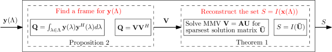
Figure 3: The fundamental stages for the recovery of the non-zero location set $S$ in an IMV model using only one finite-dimensional problem.

In the figure, $I$ indicates the joint support set of the corresponding vectors.

V Compressed Sensing of SI Signals

We now combine the ideas of Sections II and IV in order to develop efficient sampling strategies for a union of subspaces of the form (18). Our approach consists of filtering $x(t)$ with $p<m$ filters $s_{i}(t)$, and uniformly sampling their outputs at rate $1/T$. The design of $s_{i}(t),1\leq i\leq p$ relies on two ingredients:

1. A matrix ${{\bf A}}$ chosen such that it solves a discrete CS problem in the dimensions $m$ (vector length) and $k$ (sparsity).

2. A set of functions $h_{i}(t),1\leq i\leq m$ which can be used to sample and reconstruct the entire set of generators $a_{i}(t),1\leq i\leq m$, namely such that ${{\bf M}}_{HA}(e^{j\omega})$ is stably invertible a.e.

The matrix ${{\bf A}}$ is determined by considering a finite-dimensional CS problem where we would like to recover a $k$-sparse vector ${{\bf x}}$ of length $m$ from $p$ measurements ${{\bf y}}={{\bf A}}{{\bf x}}$. The value of $p$ can be chosen to guarantee exact recovery with combinatorial optimization, in which case $p\geq 2k$, or to lead to efficient recovery (possibly only with high probability) requiring $p>2k$. We show below that the same ${{\bf A}}$ chosen for this discrete problem can be used for analog CS. The functions $h_{i}(t)$ are chosen so that they can be used to recover $x(t)$. However, since there are $m$ such functions, this results in more measurements than actually needed.

We derive the proposed sampling scheme in three steps: First, we consider the problem of compressively measuring the vector sequence ${{\bf d}}[n]$, whose $\ell$th component is given by $d_{\ell}[n]$, where only $k$ out of the $m$ sequences $d_{\ell}[n]$ are non-zero. We show that this can be accomplished by using the matrix ${{\bf A}}$ above and IMV recovery theory. In the second step, we obtain the vector sequence ${{\bf d}}[n]$ from the given signal $x(t)$ using an appropriate filter bank of $m$ analog filters, and sampling their outputs. Finally, we merge the first two steps to arrive at a bank of $p<m$ analog filters that can compressively sample $x(t)$ directly. These steps are detailed in the $3$ ensuing subsections.

V-A Union of Discrete Sequences

We begin by treating the problem of sampling and recovering the sequence ${{\bf d}}[n]$. This can be accomplished by using the IMV model introduced in Section IV. Indeed, suppose we measure ${{\bf d}}[n]$ with a size $p\times m$ matrix ${{\bf A}}$, that allows for CS of $k$-sparse vectors of length $m$. Then, for each $n$,

$${{\bf y}}[n]={{\bf A}}{{\bf d}}[n],\quad n\in{\mathbb{Z}}.$$ (28)

The system of (28) is an IMV model: For every $n$ the vector ${{\bf d}}[n]$ is $k$-sparse. Furthermore, the infinite set of vectors $\{{{\bf d}}[n],n\in{\mathbb{Z}}\}$ has a joint sparsity pattern since at most $k$ of the sequences $d_{\ell}[n]$ are non-zero. As we described in Section IV, such a system of equations can be solved by transforming it into an equivalent MMV, whose recovery properties are determined by those of ${{\bf A}}$. Since ${{\bf A}}$ was designed such that CS techniques will work, we are guaranteed that ${{\bf d}}[n]$ can be perfectly recovered for each $n$ (or recovered with high probability). The reconstruction algorithm is depicted in Fig. 3. Note that in this case the integral in computing ${{\bf Q}}$ becomes a sum over $n$: ${{\bf Q}}=\sum_{n\in{\mathbb{Z}}}{{\bf y}}[n]{{\bf y}}^{H}[n]$ (we assume here that the sum exists).

Instead of solving (28) we may also consider the Frequency-domain set of equations:

$${{\bf y}}(e^{j\omega})={{\bf A}}{{\bf d}}(e^{j\omega}),\quad 0\leq\omega<2\pi,$$ (29)

where ${{\bf y}}(e^{j\omega}),{{\bf d}}(e^{j\omega})$ are the vectors whose components are the frequency responses $Y_{\ell}(e^{j\omega}),D_{\ell}(e^{j\omega})$. In principle, we may apply the CTF block of Fig. 3 to either representations, depending on which choice offers a simpler method for determining a basis ${{\bf V}}$ for the range of $\{{{\bf y}}(\Lambda)\}$.

When designing the measurements (28), the only freedom we have is in choosing ${{\bf A}}$. To generalize the class of sensing operators we note that ${{\bf d}}[n]$ can also be recovered from

$${{\bf y}}(e^{j\omega})={{\bf W}}(e^{j\omega}){{\bf A}}{{\bf d}}(e^{j\omega}),\quad 0\leq\omega<2\pi,$$ (30)

for any invertible $p\times p$ matrix ${{\bf W}}(e^{j\omega})$ with elements $W_{i\ell}(e^{j\omega})$. The measurements of (30) can be obtained directly in the time domain as

$$y_{i}[n]=\sum_{\ell=1}^{p}w_{i\ell}[n]*\left(\sum_{r=1}^{m}{{\bf A}}_{\ell r}d_{r}[n]\right),\quad 1\leq i\leq p,$$ (31)

where $w_{i\ell}[n]$ is the inverse transform of $W_{i\ell}(e^{j\omega})$, and $*$ denotes the convolution operator. To recover $d_{\ell}[n]$ from ${{\bf y}}(e^{j\omega})$, we note that the modified measurements $\tilde{{{\bf y}}}(e^{j\omega})={{\bf W}}^{-1}{{(e^{j\omega})}}{{\bf y}}(e^{j\omega})$ obey an IMV model:

$$\tilde{{{\bf y}}}(e^{j\omega})={{\bf A}}{{\bf d}}(e^{j\omega}),\quad 0\leq\omega<2\pi.$$ (32)

Therefore, the CTF block can be applied to $\tilde{{{\bf y}}}{{(e^{j\omega})}}$. As in (31), we may use the CTF in the time domain by noting that

$$\tilde{y}_{i}[n]=\sum_{\ell=1}^{p}b_{i\ell}[n]*y_{\ell}[n],$$ (33)

where $b_{i\ell}[n]$ is the inverse DTFT of $B_{i\ell}(e^{j\omega})$, with ${{\bf B}}(e^{j\omega})={{\bf W}}^{-1}(e^{j\omega})$.

The extra freedom offered by choosing an arbitrary invertible matrix ${{\bf W}}{{(e^{j\omega})}}$ in (30) will be useful when we discuss analog sampling, as different choices lead to different sampling functions. In Section VI we will see an example in which a proper selection of ${{\bf W}}{{(e^{j\omega})}}$ leads to analog sampling functions that are easy to implement.

V-B Biorthogonal Expansion

The previous section established that given the ability to sample the $m$ sequences $d_{\ell}[n]$ we can recover them exactly from $p<m$ discrete-time sequences obtained via (30) or (31). Reconstruction is performed by applying the CTF block to the modified measurements either in the frequency domain (32) or in the time domain (33). The drawback is that we do not have access to $d_{\ell}[n]$ but rather we are given $x(t)$.

In Fig. 2 and Section II we have seen that the sequences $d_{\ell}[n]$ can be obtained by sampling $x(t)$ with a set of functions $h_{\ell}(t)$ for which ${{\bf M}}_{HA}{{(e^{j\omega})}}$ of (15) is stability invertible, and then filtering the sampled sequences with a multichannel discrete-time filter ${{\bf M}}_{HA}^{-1}(e^{j\omega})$. Thus, we can first apply this front-end to $x(t)$, which will produce the sequence of vectors ${{\bf d}}[n]$. We can then use the results of the previous subsection in order to sense these sequences efficiently. The resulting measurement sequences $y_{\ell}[n]$ are depicted in Fig. 4, where ${{\bf A}}$ is a $p\times m$ matrix satisfying the requirements of CS in the appropriate dimensions, and ${{\bf W}}(e^{j\omega})$ is a size $p\times p$ filter bank that is invertible a.e.

Figure 4: Analog compressed sampling with arbitrary filters $h_{i}(t)$.

Combining the analog filters $h_{\ell}(t)$ with the discrete-time multichannel filter ${{\bf M}}_{HA}^{-1}(e^{j\omega})$, we can express $d_{\ell}[n]$ as

$$d_{\ell}[n]={\langle v_{\ell}(t-nT),x(t)\rangle},\quad 1\leq\ell\leq m,n\in{\mathbb{Z}},$$ (34)

where

$${{\bf v}}(\omega)={{\bf M}}_{HA}^{-*}(e^{j\omega T}){{\bf h}}(\omega).$$ (35)

Here ${{\bf v}}(\omega),{{\bf h}}(\omega)$ are the vectors with $\ell$th elements $V_{\ell}(\omega),H_{\ell}(\omega)$ and $(\cdot)^{-*}$ denotes the conjugate of the inverse. The inner products in (34) can be obtained by filtering $x(t)$ with the bank of filters $v^{*}_{\ell}(-t)$, and uniformly sampling the outputs at times $nT$.

To see that (34) holds, let $c_{\ell}[n]$ be the samples resulting from filtering $x(t)$ with the $m$ filters $v_{\ell}(t)$ and uniformly sampling their outputs at rate $1/T$. From Proposition 1,

$${{\bf c}}(e^{j\omega})={{\bf M}}_{VA}(e^{j\omega}){{\bf d}}{{(e^{j\omega})}}.$$ (36)

Therefore, to establish (34) we need to show that ${{\bf M}}_{VA}(e^{j\omega})={{\bf I}}$. Now, from (15),

$$[{{\bf M}}_{VA}(e^{j\omega})]_{i\ell}=\frac{1}{T}\sum_{k\in{\mathbb{Z}}}V^{*}_{i}\left(\frac{\omega}{T}-\frac{2\pi}{T}k\right)A_{\ell}\left(\frac{\omega}{T}-\frac{2\pi}{T}k\right)$$ (37)

$$= \frac{1}{T}\sum_{r=1}^{m}[{{\bf M}}^{-1}_{HA}(e^{j\omega})]_{ir}\sum_{k\in{\mathbb{Z}}}H_{r}^{*}\left(\frac{\omega}{T}-\frac{2\pi}{T}k\right)A_{\ell}\left(\frac{\omega}{T}-\frac{2\pi}{T}k\right)$$

$$= [{{\bf M}}_{HA}^{-1}(e^{j\omega})]^{i}[{{\bf M}}_{HA}(e^{j\omega})]_{\ell}={{\bf I}}_{i\ell},$$

where $[{{\bf Q}}]_{ir}$ is the $ir$th element of the matrix ${{\bf Q}}$, and $[{{\bf Q}}]^{i},[{{\bf Q}}]_{i}$ are the $i$th row and column respectively of ${{\bf Q}}$. Therefore, as required, ${{\bf M}}_{VA}(e^{j\omega})={{\bf I}}$.

The functions $\{v_{\ell}(t-nT)\}$ have the property that they are biorthogonal to $\{a_{\ell}(t-nT)\}$, that is

$${\langle v_{\ell}(t-nT),a_{i}(t-rT)\rangle}=\delta_{\ell i}\delta_{nr},$$ (38)

where $\delta_{\ell i}=1$ if $\ell=i$, and $0$ otherwise. This follows from the fact that in the Fourier domain, (38) is equivalent to

$${{\bf M}}_{VA}{{(e^{j\omega})}}={{\bf I}}.$$ (39)

Evidently, we can construct a set of biorthogonal functions from any set of functions $h_{\ell}(t)$ for which ${{\bf M}}_{HA}{{(e^{j\omega})}}$ is stably invertible, via (35). Note that the biorthogonal vectors in the space ${\mathcal{A}}$ are unique. This follows from the fact that if two sets $\{v_{i}^{1}(t)\},\{v_{i}^{2}(t)\}$ satisfy (38), then

$${\langle g_{\ell}(t-nT),a_{i}(t-rT)\rangle}=0,\quad\mbox{for all }\ell,i,n,r,$$ (40)

where $g_{i}(t)=v_{i}^{1}(t)-v_{i}^{2}(t)$. Since $\{a_{i}(t-nT)\}$ span ${\mathcal{A}}$, (40) implies that $g_{i}(t-mT)$ lies in ${\mathcal{A}}^{\perp}$ for any $i,m$. However, if both $v_{i}^{1}(t)$ and $v_{i}^{2}(t)$ are in ${\mathcal{A}}$, then so is $g_{i}(t-mT)$, from which we conclude that $g_{i}(t-mT)=0$. Thus, as long as we start with a set of functions $h_{i}(t)$ that span ${\mathcal{A}}$, the sampling functions $v_{i}(t)$ resulting from (35) will be the same. However, their implementation in hardware is different, since $h_{i}(t)$ represents an analog filter while ${{\bf M}}_{HA}{{(e^{j\omega})}}$ is a discrete-time filter bank. Therefore, different choices of $h_{i}(t)$ lead to distinct analog filters.

V-C CS of Analog Signals

Although the sampling scheme of Fig. 4 results in compressed measurements $y_{\ell}[n]$, they are still obtained by an analog front-end that operates at the high rate $m/T$. However, our goal is to reduce the rate at the analog front-end. This can be easily accomplished by moving the discrete filters ${{\bf M}}_{HA}^{-1}(e^{j\omega})$, ${{\bf A}}{{\bf W}}(e^{j\omega})$ back to the analog domain. In this way, the compressed measurement sequences $y_{\ell}[n]$ can be obtained directly from $x(t)$, by filtering $x(t)$ with $p$ filters $s_{\ell}(t)$ and uniformly sampling their outputs at times $nT$, leading to a system with sampling rate $p/T$. An explicit expression for the resulting sampling functions is given in the following theorem.

Theorem 2

Let the compressed measurements $y_{\ell}[n],1\leq\ell\leq p$ be the output of the hybrid filter bank in Fig. 4. Then $\{y_{\ell}[n]\}$ can be obtained by filtering $x(t)$ of (18) with $p$ filters $\{s^{*}_{\ell}(-t)\}$ and sampling the outputs at rate $1/T$, where

$${{\bf s}}(\omega) = {{\bf W}}^{*}(e^{j\omega T}){{\bf A}}^{*}{{\bf v}}(\omega)$$ (41)

$$= {{\bf W}}^{*}(e^{j\omega T}){{\bf A}}^{*}{{\bf M}}_{HA}^{-*}(e^{j\omega T}){{\bf h}}(\omega).$$

Here ${{\bf s}}(\omega),{{\bf h}}(\omega)$ are the vectors with $\ell$th elements $S_{\ell}(\omega),H_{\ell}(\omega)$ respectively, and the components $V_{\ell}(\omega)$ of ${{\bf v}}(\omega)={{\bf M}}_{HA}^{-*}(e^{j\omega T}){{\bf h}}(\omega)$ are Fourier transforms of generators $v_{\ell}(t)$ such that $\{v_{\ell}(t-nT)\}$ are biorthogonal to $\{a_{\ell}(t-nT)\}$. In the time domain,

$$s_{i}(t)=\sum_{\ell=1}^{m}\sum_{r=1}^{p}\sum_{n\in{\mathbb{Z}}}w^{*}_{ir}[-n]{{\bf A}}^{*}_{r\ell}v_{\ell}(t-nT),$$ (42)

where $w_{ir}[n]$ is the inverse transform of $[{{\bf W}}{{(e^{j\omega})}}]_{ir}$ and

$$v_{i}(t)=\sum_{\ell=1}^{m}\sum_{n\in{\mathbb{Z}}}\psi^{*}_{i\ell}[-n]h_{\ell}(t-nT),$$ (43)

where $\psi_{i\ell}[n]$ is the inverse transform of $[{{\bf M}}_{HA}^{-1}{{(e^{j\omega})}}]_{i\ell}$.

Proof:

Suppose that $x(t)$ is filtered by the $p$ filters $s_{i}(t)$ and then uniformly sampled at $nT$. From Proposition 1, the samples can be expressed in the Fourier domain as

$${{\bf c}}(e^{j\omega})={{\bf M}}_{SA}(e^{j\omega}){{\bf d}}{{(e^{j\omega})}}.$$ (44)

In order to prove the theorem we need to show that ${{\bf M}}_{SA}{{(e^{j\omega})}}={{\bf W}}{{(e^{j\omega})}}{{\bf A}}$.

Let

$${{\bf B}}{{(e^{j\omega})}}={{\bf W}}^{*}(e^{j\omega}){{\bf A}}^{*},$$ (45)

so that ${{\bf s}}(\omega)={{\bf B}}(e^{j\omega T}){{\bf v}}(\omega)$. Then,

$$[{{\bf M}}_{SA}(e^{j\omega})]_{i\ell}=\frac{1}{T}\sum_{k\in{\mathbb{Z}}}S^{*}_{i}\left(\frac{\omega}{T}-\frac{2\pi}{T}k\right)A_{\ell}\left(\frac{\omega}{T}-\frac{2\pi}{T}k\right)$$ (46)

$$= \frac{1}{T}\sum_{r=1}^{m}B_{ir}^{*}(e^{j\omega})\sum_{k\in{\mathbb{Z}}}V_{r}^{*}\left(\frac{\omega}{T}-\frac{2\pi}{T}k\right)A_{\ell}\left(\frac{\omega}{T}-\frac{2\pi}{T}k\right)$$

$$= [{{\bf B}}^{*}(e^{j\omega})]^{i}[{{\bf M}}_{VA}(e^{j\omega})]_{\ell},$$

where $[{{\bf Q}}]^{i},[{{\bf Q}}]_{i}$ are the $i$th row and column respectively of the matrix ${{\bf Q}}$. The first equality follows from the fact that ${{\bf B}}{{(e^{j\omega})}}$ is $2\pi$ periodic. From (46),

$${{\bf M}}_{SA}(e^{j\omega})={{\bf B}}^{*}(e^{j\omega}){{\bf M}}_{VA}(e^{j\omega})={{\bf W}}(e^{j\omega}){{\bf A}},$$ (47)

where we used the fact that ${{\bf M}}_{VA}(e^{j\omega})={{\bf I}}$ due to the biorthogonality property.

Finally, if ${{\bf s}}(\omega)={{\bf B}}(e^{j\omega T}){{\bf v}}(\omega)$, then

$$s_{i}(t)=\sum_{\ell=1}^{m}\sum_{n\in{\mathbb{Z}}}b_{i\ell}[n]v_{\ell}(t-nT),$$ (48)

where $b_{i\ell}[n]$ is the inverse DTFT of $[B_{i\ell}{{(e^{j\omega})}}]_{i\ell}$. Using (45) together with the fact that the inverse transform of $Q^{*}_{i\ell}{{(e^{j\omega})}}$ is $q^{*}_{i\ell}[-n]$, results in (42). The relation (43) follows from the same considerations. ∎

Theorem 2 is the main result which allows for compressive sampling of analog signals. Specifically, starting from any matrix ${{\bf A}}$ that satisfies the CS requirements of finite vectors, and a set of sampling functions $h_{i}(t)$ for which ${{\bf M}}_{HA}{{(e^{j\omega})}}$ is invertible, we can create a multitude of sampling functions $s_{i}(t)$ to compressively sample the underlying analog signal $x(t)$. The sensing is performed by filtering $x(t)$ with the $p<m$ corresponding filters, and sampling their outputs at rate $1/T$. Reconstruction from the compressed measurements $y_{i}[n],1\leq i\leq p$ is obtained by applying the CTF block of Fig. 3 in order to recover the sequences $d_{i}[n]$. The original signal $x(t)$ is then constructed by modulating appropriate impulse trains and filtering with $a_{i}(t)$, as depicted in Fig. 5.

Figure 5: Compressed sensing of analog signals. The sampling functions $s_{i}(t)$ are obtained by combining the blocks in Fig. 4 and are given in Theorem 2.

As a final comment, we note that we may add an invertible diagonal matrix ${{\bf Z}}{{(e^{j\omega})}}$ prior to multiplication by ${{\bf A}}$. Indeed, in this case the measurements are given by

$${{\bf y}}(e^{j\omega})={{\bf W}}{{(e^{j\omega})}}{{\bf A}}{{\bf Z}}(e^{j\omega}){{\bf d}}(e^{j\omega})={{\bf A}}\tilde{{{\bf d}}}(e^{j\omega}),$$ (49)

where $\tilde{{{\bf d}}}(e^{j\omega})$ has the same sparsity profile as ${{\bf d}}(e^{j\omega})$. Therefore, $\tilde{{{\bf d}}}{{(e^{j\omega})}}$ can be recovered using the CTF block. In order to reconstruct $x(t)$, we first filter each of the non-zero sequences $\tilde{d}_{i}[n]$ with the convolutional inverse of $Z_{i}(e^{j\omega})$.

In this section we discussed the basic elements that allow recovery from compressed analog signals: we first use a biorthogonal sampling set in order to access the coefficient sequences, and then employ a conventional CS mixing matrix to compress the measurements. Recovery is possible by using an IMV model and applying the CTF block of Fig. 3 either in time or in frequency. In practical applications we have the freedom to choose ${{\bf W}}{{(e^{j\omega})}}$ and ${{\bf A}}$ so that we end up with analog sampling functions that are easy to implement. Two examples are considered in the next section.

VI Examples

VI-A Periodic Sparsity

Suppose that we are given a signal $x(t)$ that lies in a SI subspace generated by $a(t)$ so that $x(t)=\sum_{n\in{\mathbb{Z}}}d[n]a(t-nT^{\prime})$. The coefficients $d[n]$ have a periodic sparsity pattern: Out of each consecutive group of $m$ coefficients, there are at most $k$ non-zero values, in a given pattern. For example, suppose that $m=7,k=2$ and the sparsity profile is $S=\{1,4\}$. Then $d[n]$ can be non-zero only at indices $n=1+7\ell$ or $n=4+7\ell$ for some integer $\ell$. Decomposing $d[n]$ into blocks ${{\bf d}}[n]$ of length $m$, the sparsity pattern of $x(t)$ implies that the vectors $\{{{\bf d}}[n]\}$ are jointly $k$-sparse.

Since $x(t)$ lies in a SI subspace spanned by a single generator, we can sample it by first prefiltering with the filter

$$Q(\omega)=\frac{1}{\phi_{HA}(e^{j\omega T^{\prime}})}H(\omega),$$ (50)

where $h(t)$ is any function such that $\phi_{HA}{{(e^{j\omega})}}$ defined by (4) is non-zero a.e. on $\omega$, and then sampling the output at rate $1/T^{\prime}$, as in Fig. 1. With this choice, the samples $c[n]={\langle q(t-nT^{\prime}),x(t)\rangle}$ are equal to the unknown coefficients $d[n]$. We may then use standard CS techniques to compressively sample $d[n]$. For example, we can sample $d[n]$ sequentially by considering blocks ${{\bf d}}[n]$ of length $m$, and using a standard CS matrix ${{\bf A}}$ designed to sample a $k$-sparse vector of length-$m$. Alternatively, we can exploit the joint sparsity by combining several blocks and sampling them together using MMV techniques, or applying the IMV method of Section IV. However, these approaches still require an analog sampling rate of $1/T^{\prime}$. Thus, the rate reduction is only in discrete time, whereas the analog sampling rate remains at the Nyquist rate. Since many of the coefficients are zero, we would like to directly reduce the analog rate so as not to acquire the zero values of $d[n]$, rather than acquiring them first, and then compressing in discrete time.

To this end, we note that our problem may be viewed as a special case of the general model (18) with $a_{i}(t)=a(t-(i-1)),1\leq i\leq m$ and $d_{i}[n]=d[i+nT],1\leq i\leq m$ with $T=mT^{\prime}$. Therefore, the rate can be reduced by using the tools of Section V. From Theorem 2, we first need to construct a set of functions $\{v_{\ell}(t-nT)\}$ that are biorthogonal to $\{a_{\ell}(t-nT)\}$. It is easy to see that

$$v_{\ell}(t)=q(t-(\ell-1)),\quad 1\leq\ell\leq m,$$ (51)

with $Q(\omega)$ given by (50) constitute a biorthogonal set. Indeed, with this choice

$$[{{\bf M}}_{VA}{{(e^{j\omega})}}]_{i\ell}=\frac{1}{T}e^{j(i-\ell)\omega/T}\cdot$$ (52)

$$\sum_{k\in{\mathbb{Z}}}e^{-j(i-\ell)2\pi k/T}Q^{*}\left(\frac{\omega}{T}-\frac{2\pi}{T}k\right)A\left(\frac{\omega}{T}-\frac{2\pi}{T}k\right)$$

$$=\frac{1}{T}e^{j(i-\ell)\omega/T}\sum_{r=0}^{T-1}e^{-j(i-\ell)2\pi r/T}G(e^{j(\omega-2\pi r)/T}),$$

where we defined

$$G(e^{j\omega})=\frac{1}{T}\sum_{k\in{\mathbb{Z}}}Q^{*}\left(\omega-2\pi k\right)A\left(\omega-2\pi k\right).$$ (53)

From (50), $G(e^{j\omega})=1$. Combining this with the relation

$$\frac{1}{T}\sum_{r=0}^{T-1}e^{-j2\pi rm/T}=\delta[m],$$ (54)

it follows from (52) that ${{\bf M}}_{VA}{{(e^{j\omega})}}={{\bf I}}$.

We now use Theorem 2 to conclude that any sampling functions of the form ${{\bf s}}(\omega)={{\bf W}}^{*}(e^{j\omega T}){{\bf A}}^{*}{{\bf v}}(\omega)$ with $V_{\ell}(\omega)=Q(\omega)e^{-j(\ell-1)\omega}$ and $Q(\omega)$ given by (50) can be used to compressively sample the signal at a rate $p/T=p/(mT^{\prime})<1/T^{\prime}$. In particular, given a matrix ${{\bf A}}$ of size $p\times m$ that satisfies the CS requirements, we may choose sampling functions

$$s_{i}(t)=\sum_{\ell=1}^{m}{{\bf A}}^{*}_{i\ell}q(t-(\ell-1)),\quad 1\leq i\leq p.$$ (55)

In this strategy, each sample is equal to a linear combination of several values $d[n]$, in contrast to the high-rate method in which each sample is exactly equal $d[n]$.

As a special case, suppose that $T^{\prime}=1$, $a(t)=1$ on the interval $[0,1]$ and is zero otherwise. Thus, $x(t)$ is piecewise constant over intervals of length $1$. Choosing $h(t)=a(t)$ in (50) it follows that $q(t)=1$. This is because $r_{aa}[n]={\langle a(t-n),a(t)\rangle}=\delta[n]$ so that $\phi_{AA}{{(e^{j\omega})}}=1$. Therefore, $v_{\ell}(t)=a(t-(\ell-1))$ are biorthogonal to $a_{\ell}(t)$. One way to acquire the coefficients $d[n]$ is to filter the signal $x(t)$ with $v(t)=a(t)$ and sample the output at rate $1$. This corresponds to integrating $x(t)$ over intervals of length one. Since $x(t)$ has a constant value $d[n]$ over the $n$th interval, the output will indeed be the sequence $d[n]$. To reduce the rate, we may instead use the $p<m$ sampling functions (55) and sample the output at rate $1/m$. This is equivalent to first multiplying $x(t)$ by $p$ periodic sequences with period $m$. Each sequence is piecewise constant over intervals of length $1$ with values ${{\bf A}}_{i\ell},1\leq\ell\leq m$. The continuous output is then integrated over intervals of length $m$ to produce the samples $y_{\ell}[n]$. Applying the CTF block to these measurements allows to recover $d[n]$. Although this special case is rather simple, it highlights the main idea. Furthermore, the same techniques can be used even when the generator $a(t)$ has infinite length.

VI-B Multiband Sampling

Consider next the multiband sampling problem [21, 23] in which we have a complex signal that consists of at most $N$ frequency bands, each of length no larger than $B$. In addition, the signal is bandlimited to $2\pi/T$. If the band locations are known, then we can recover such a signal from nonuniform samples at an average rate of $NB/(2\pi)$ which is typically much smaller than the Nyquist rate $2\pi/T$ [18, 19, 20]. When the band locations are unknown, the problem is much more complicated. In [21] it was shown that the minimum sampling rate for such signals is $NB/\pi$. Furthermore, explicit algorithms were developed which achieve this rate. Here we illustrate how this problem can be formulated within our framework.

Dividing the frequency interval $[0,2\pi/T)$ into $m$ sections, each of equal length $2\pi/(mT)$, it follows that if $m\leq 2\pi/(BT)$ then each band comprising the signal is contained in no more than $2$ intervals. Since there are $N$ bands, this implies that at most $2N$ sections contain energy. To fit this problem into our general model, let

$$A_{i}(\omega)=\sqrt{mT}A\left(\omega-\frac{2\pi(i-1)}{mT}\right),\quad 1\leq i\leq m,$$ (56)

where $A(\omega)$ is a low-pass filter (LPF) on $[0,2\pi/(mT))$. Thus, $A_{i}(\omega)$ describes the support of the $i$th interval. Since any multiband signal $x(t)$ is supported in the frequency domain over at most $2N$ sections, $x(t)$ can be written as

$$X(\omega)=\sum_{i=1}^{m}A_{i}(\omega)D_{i}(\omega),$$ (57)

for some $D_{i}(\omega)$ supported on the $i$th interval, where at most $2N$ functions are nonzero. Since the support of $D_{i}(\omega)$ has length $2\pi/(mT)$, it can be written as a Fourier series

$$D_{i}(\omega)=\sum_{n\in{\mathbb{Z}}}d_{i}[n]e^{-j\omega nmT}{\,\stackrel{{\scriptstyle\triangle}}{{=}}}\,D_{i}(e^{j\omega mT}).$$ (58)

Thus, our signal fits the general model (18), where there are at most $2N$ sequences $d_{i}[n]$ that are nonzero.

We now use our general results to obtain sampling functions that can be used to sample and recover such signals at rates lower than Nyquist. One possibility is to choose $h_{i}(t)=a_{i}(t)$. Since the functions $a_{i}(t)$ are orthonormal (as is evident by considering the frequency domain representation), we have that ${{\bf M}}_{HA}{{(e^{j\omega})}}={{\bf M}}_{AA}{{(e^{j\omega})}}={{\bf I}}$. Consequently, the resulting sampling functions are

$$s_{i}(t)=\sum_{\ell=1}^{m}{{\bf A}}_{i\ell}^{*}a_{\ell}(t).$$ (59)

In the Fourier domain, $S_{i}(\omega)$ is bandlimited to $2\pi/T$ and piecewise constant with values $\sqrt{mT}{{\bf A}}_{i\ell}^{*}$ over intervals of length $2\pi/(mT)$.

Alternative sampling functions are those used in [21]:

$$s_{i}(t)=\delta(t-c_{i}T),\quad 1\leq i\leq p,$$ (60)

where $\{c_{i}\}$ are $p$ distinct integer values in the range $1\leq c_{i}\leq m$. Since $x(t)$ is bandlimited, sampling with the filters (60) is equivalent to using the bandlimited functions

$$S_{i}(\omega)=e^{-jc_{i}\omega T},\quad 0\leq\omega\leq\frac{2\pi}{T}.$$ (61)

To show that these filters can be obtained from our general framework incorporated in Theorem 2, we need to choose a $p\times m$ matrix ${{\bf A}}$ and an invertible $p\times p$ matrix ${{\bf W}}{{(e^{j\omega})}}$ such that $G_{i}(\omega)=S_{i}(\omega)$ where

$${{\bf g}}(\omega)={{\bf W}}^{*}(e^{j\omega mT}){{\bf A}}^{*}{{\bf v}}(\omega),$$ (62)

and ${{\bf v}}(\omega)$ represents a biorthogonal set. In our setting, we can choose $V_{i}(\omega)=A_{i}(\omega)$ due to the orthogonality of $a_{i}(t)$.

Let ${{\bf A}}$ be the matrix consisting of the rows $c_{i},1\leq i\leq p$ of the $m\times m$ Fourier matrix

$${{\bf A}}_{i\ell}=\frac{1}{\sqrt{m}}e^{j2\pi(\ell-1)c_{i}/m},$$ (63)

and choose ${{\bf W}}{{(e^{j\omega})}}$ as a diagonal matrix with $i$th diagonal element

$$W_{i}{{(e^{j\omega})}}=\frac{1}{\sqrt{T}}e^{jc_{i}\omega/m},\quad 0\leq\omega<2\pi.$$ (64)

From (62),

$$G_{i}(\omega)=W_{i}^{*}(e^{j\omega mT})\sum_{\ell=1}^{m}{{\bf A}}_{i\ell}^{*}A_{\ell}(\omega).$$ (65)

Since $A_{\ell}(\omega)$ is equal to $\sqrt{mT}$ over the $\ell$th interval $[(\ell-1)2\pi/(mT),\ell 2\pi/mT)$ and $0$ otherwise, $\sum_{\ell=1}^{m}{{\bf A}}_{i\ell}^{*}A_{\ell}(\omega)$ is piecewise constant with values equal to $\sqrt{mT}{{\bf A}}_{i\ell}^{*}$ on intervals of length $2\pi/(mT)$. In addition, on the $\ell$th interval,

$$W_{i}^{*}(e^{j\omega mT}) = \frac{1}{\sqrt{T}}e^{-jc_{i}T(\omega-(\ell-1)2\pi/(mT))}$$ (66)

$$= (\sqrt{m}/\sqrt{T})e^{-jc_{i}\omega T}{{\bf A}}_{i\ell}.$$

Consequently, on this interval, $G_{i}(\omega)$ is equal to $\sqrt{mT}W_{i}^{*}(e^{j\omega mT}){{\bf A}}^{*}_{i\ell}=e^{-jc_{i}\omega T}$. Since this expression does not depend on $\ell$, $G_{i}(\omega)=S_{i}(\omega)$ for $0\leq\omega\leq 2\pi/T$.

From our general results, in order to recover the original signal $x(t)$ we need to apply the CTF to the modified measurements $\tilde{{{\bf y}}}{{(e^{j\omega})}}={{\bf W}}^{-1}{{(e^{j\omega})}}{{\bf y}}{{(e^{j\omega})}}$. Since ${{\bf W}}{{(e^{j\omega})}}$ is diagonal, the DTFT of the $i$th sequence $\tilde{y}_{i}[n]$ is given by

$$\tilde{Y}_{i}{{(e^{j\omega})}}=\frac{1}{\sqrt{T}}e^{-jc_{i}\omega/m}Y_{i}{{(e^{j\omega})}},\quad 0\leq\omega\leq 2\pi.$$ (67)

This corresponds to a scaled non-integer delay $c_{i}/m$ of $y_{i}[n]$. Such a delay can be realized by first upsampling the sequence $y_{i}[n]$ by factor of $m$, low-pass filtering with a LPF with cut-off $\pi/m$, shifting the resulting sequence by $c_{i}$, and then down sampling by $m$. This coincides with the approach suggested in [21] for applying the CTF directly in the time domain. Here we see that this processing follows directly from our general framework.

We have shown that a particular choice of ${{\bf A}}$ and ${{\bf W}}{{(e^{j\omega})}}$ results in the sampling strategy of [21]. Alternative selections can lead to a variety of different sampling functions for the same problem. The added value in this context is that in [21] there is no discussion on what type of sampling methods lead to stable recovery. The framework we developed in this paper can be applied in this specific setting to suggest more general types of stable sampling and recovery strategies.

VII Conclusion

We developed a general framework to treat sampling of sparse analog signals. We focused on signals in a SI space generated by $m$ kernels, where only $k$ out of the $m$ generators are active. The difficulty arises from the fact that we do not know in advance which $k$ are chosen. Our approach was based on merging ideas from standard analog sampling, with results from the emerging field of CS. The latter focuses on sensing finite-dimensional vectors that have a sparsity structure in some transform domain. Although our problem is inherently infinite-dimensional, we showed that by using the notion of biorthogonal sampling sets and the recently developed CTF block [38, 21], we can convert our problem to a finite-dimensional counterpart that takes on the form of an MMV, a problem which has been treated previously in the CS literature.

In this paper, we focused on sampling using a bank of analog filters. An interesting future direction to pursue is to extend these ideas to other sampling architectures that may be easier to implement in hardware.

As a final note, most of the literature to date on the exciting field of CS has focused on sensing of finite-dimensional vectors. On the other hand, traditional sampling theory focuses on infinite-dimensional continuous-time signals. It is our hope that this work can serve as a step in the direction of merging these two important areas in sampling, leading to a more general notion of compressive sampling.

VIII Acknowledgement

The author would like to thank Moshe Mishali for many fruitful discussions, and the reviewers for useful comments on the manuscript which helped improve the exposition.

References

- [1] C. E. Shannon, “Communications in the presence of noise,” Proc. IRE, vol. 37, pp. 10–21, Jan 1949.
- [2] H. Nyquist, “Certain topics in telegraph transmission theory,” EE Trans., vol. 47, pp. 617–644, Jan. 1928.
- [3] I. Daubechies, “The wavelet transform, time-frequency localization and signal analysis,” IEEE Trans. Inform. Theory, vol. 36, pp. 961–1005, Sep. 1990.
- [4] M. Unser, “Sampling—50 years after Shannon,” IEEE Proc., vol. 88, pp. 569–587, Apr. 2000.
- [5] A. Aldroubi and M. Unser, “Sampling procedures in function spaces and asymptotic equivalence with Shannon’s sampling theory,” Numer. Funct. Anal. Optimiz., vol. 15, pp. 1–21, Feb. 1994.
- [6] M. Unser and A. Aldroubi, “A general sampling theory for nonideal acquisition devices,” IEEE Trans. Signal Processing, vol. 42, no. 11, pp. 2915–2925, Nov. 1994.
- [7] P. P. Vaidyanathan, “Generalizations of the sampling theorem: Seven decades after Nyquist,” IEEE Trans. Circuit Syst. I, vol. 48, no. 9, pp. 1094–1109, Sep. 2001.
- [8] Y. C. Eldar, “Sampling and reconstruction in arbitrary spaces and oblique dual frame vectors,” J. Fourier Analys. Appl., vol. 1, no. 9, pp. 77–96, Jan. 2003.
- [9] Y. C. Eldar and T. G. Dvorkind, “A minimum squared-error framework for generalized sampling,” IEEE Trans. Signal Processing, vol. 54, no. 6, pp. 2155–2167, Jun. 2006.
- [10] T. G. Dvorkind, Y. C. Eldar, and E. Matusiak, “Nonlinear and non-ideal sampling: Theory and methods,” IEEE Trans. Signal Processing, vol. 56, no. 12, pp. 5874–5890, Dec. 2008.
- [11] Y. C. Eldar and T. Michaeli, “Beyond bandlimited sampling: Nonlinearities, smoothness and sparsity,” to appear in IEEE Signal Proc. Magazine.
- [12] C. de Boor, R. DeVore, and A. Ron, “The structure of finitely generated shift-invariant spaces in ,” J. Funct. Anal, vol. 119, no. 1, pp. 37–78, 1994.
- [13] J. S. Geronimo, D. P. Hardin, and P. R. Massopust, “Fractal functions and wavelet expansions based on several scaling functions,” Journal of Approximation Theory, vol. 78, no. 3, pp. 373–401, 1994.
- [14] O. Christansen and Y. C. Eldar, “Oblique dual frames and shift-invariant spaces,” Appl. Comp. Harm. Anal., vol. 17, no. 1, pp. 48–68, 2004.
- [15] O. Christensen and Y. C. Eldar, “Generalized shift-invariant systems and frames for subspaces,” J. Fourier Analys. Appl., vol. 11, pp. 299–313, 2005.
- [16] A. Aldroubi and K. Gröchenig, “Non-uniform sampling and reconstruction in shift-invariant spaces,” Siam Review, vol. 43, pp. 585–620, 2001.
- [17] I. J. Schoenberg, Cardinal Spline Interpolation, Philadelphia, PA: SIAM, 1973.
- [18] Y.-P. Lin and P. P. Vaidyanathan, “Periodically nonuniform sampling of bandpass signals,” IEEE Trans. Circuits Syst. II, vol. 45, no. 3, pp. 340–351, Mar. 1998.
- [19] C. Herley and P. W. Wong, “Minimum rate sampling and reconstruction of signals with arbitrary frequency support,” IEEE Trans. Inform. Theory, vol. 45, no. 5, pp. 1555–1564, July 1999.
- [20] R. Venkataramani and Y. Bresler, “Perfect reconstruction formulas and bounds on aliasing error in sub-nyquist nonuniform sampling of multiband signals,” IEEE Trans. Inform. Theory, vol. 46, no. 6, pp. 2173–2183, Sep. 2000.
- [21] M. Mishali and Y. C. Eldar, “Blind multi-band signal reconstruction: Compressed sensing for analog signals,” IEEE Trans. Signal Process., vol. 57, pp. 993–1009, Mar. 2009.
- [22] M. Mishali and Y. C. Eldar, “Spectrum-blind reconstruction of multi-band signals,” in Proc. Int. Conf. Acoust., Speech, Signal Processing (ICASSP-2008), (Las Vegas, USA), April 2008, pp. 3365–3368.
- [23] M. Mishali and Y. C. Eldar, “From theory to practice: Sub-Nyquist sampling of sparse wideband analog signals,” arXiv 0902.4291; submitted to IEEE Selcted Topics on Signal Process., 2009.
- [24] Y. M. Lu and M. N. Do, “A theory for sampling signals from a union of subspaces,” IEEE Trans. Signal Processing, vol. 56, no. 6, pp. 2334–2345, 2008.
- [25] T. Blumensath and M. E. Davies, “Sampling theorems for signals from the union of finite-dimensional linear subspaces,” IEEE Trans. Inform. Theory, to appear.
- [26] Y. C. Eldar and M. Mishali, “Robust recovery of signals from a union of subspaces,” submitted to IEEE Trans. Inform. Theory, July 2008.
- [27] D. L. Donoho, “Compressed sensing,” IEEE Trans. on Inf. Theory, vol. 52, no. 4, pp. 1289–1306, Apr 2006.
- [28] E. J. Candès, J. Romberg, and T. Tao, “Robust uncertainty principles: Exact signal reconstruction from highly incomplete frequency information,” IEEE Trans. Inform. Theory, vol. 52, no. 2, pp. 489–509, Feb. 2006.
- [29] S. G. Mallat and Z. Zhang, “Matching pursuits with time-frequency dictionaries,” IEEE Trans. Signal Processing, vol. 41, no. 12, pp. 3397–3415, Dec. 1993.
- [30] S. S. Chen, D. L. Donoho, and M. A. Saunders, “Atomic decomposition by basis pursuit,” SIAM J. Scientific Computing, vol. 20, no. 1, pp. 33– 61, 1999.
- [31] I. F. Gorodnitsky, J. S. George, and B. D. Rao, “Neuromagnetic source imaging with FOCUSS: A recursive weighted minimum norm algorithm,” J. Electroencephalog. Clinical Neurophysiol., vol. 95, no. 4, pp. 231 –251, Oct. 1995.
- [32] D. L. Donoho and M. Elad, “Maximal sparsity representation via minimization,” Proc. Natl. Acad. Sci., vol. 100, pp. 2197– 2202, Mar. 2003.
- [33] E. J. Candès and T. Tao, “Decoding by linear programming,” IEEE Trans. Inform. Theory, vol. 51, no. 12, pp. 4203–4215, Dec. 2005.
- [34] J. A. Tropp, M. B. Wakin, M. F. Duarte, D. Baron, and R. G. Baraniuk, “Random filters for compressive sampling and reconstruction,” in Proc. IEEE International Conference on Acoustics, Speech and Signal Processing ICASSP 2006, May 2006, vol. 3.
- [35] J. N. Laska, S. Kirolos, M. F. Duarte, T. S. Ragheb, R. G. Baraniuk, and Y. Massoud, “Theory and implementation of an analog-to-information converter using random demodulation,” in Proc. IEEE International Symposium on Circuits and Systems ISCAS 2007, May 2007, pp. 1959–1962.
- [36] M. Vetterli, P. Marziliano, and T. Blu, “Sampling signals with finite rate of innovation,” IEEE Trans. Signal Processing, vol. 50, pp. 1417–1428, June 2002.
- [37] P.L. Dragotti, M. Vetterli, and T. Blu, “Sampling moments and reconstructing signals of finite rate of innovation: Shannon meets Strang-Fix,” IEEE Trans. Sig. Proc., vol. 55, no. 5, pp. 1741–1757, May 2007.
- [38] M. Mishali and Y. C. Eldar, “Reduce and boost: Recovering arbitrary sets of jointly sparse vectors,” IEEE Trans. Signal Process., vol. 56, no. 10, pp. 4692–4702, Oct. 2008.
- [39] Y. C. Eldar and O. Christansen, “Characterization of oblique dual frame pairs,” J. Applied Signal Processing, pp. 1–11, 2006, Article ID 92674.
- [40] J. Chen and X. Huo, “Theoretical results on sparse representations of multiple-measurement vectors,” IEEE Trans. Signal Processing, vol. 54, no. 12, pp. 4634–4643, Dec. 2006.
- [41] J. B. Kruskal, “Three-way arrays: Rank and uniqueness of trilinear decompositions, with application to arithmetic complexity and statistics,” Linear Alg. Its Applic., vol. 18, no. 2, pp. 95–138, 1977.
- [42] E. J. Candès, “The restricted isometry property and its implications for compressed sensing,” C. R. Acad. Sci. Paris, Ser. I, vol. 346, pp. 589–592, 2008.
- [43] E. J. Candès and J. Romberg, “Sparsity and incoherence in compressive sampling,” Inverse Prob., vol. 23, no. 3, pp. 969–985, 2007.
- [44] S. F. Cotter, B. D. Rao, K. Engan, and K. Kreutz-Delgado, “Sparse solutions to linear inverse problems with multiple measurement vectors,” IEEE Trans. Signal Processing, vol. 53, no. 7, pp. 2477–2488, July 2005.