Probing microscopic origins of confined subdiffusion by first-passage observables.

^⋆ To whom correspondence should be addressed. E-mail: benichou@lptmc.jussieu.fr

Classification
PHYSICAL SCIENCES, physics

Corresponding author
Olivier Bénichou
LPTMC, Université Paris 6
case courrier 121, 4 Place Jussieu, 75255 Paris Cedex 05
Tel: + 33 1 44 27 25 29
Fax: + 33 1 44 27 51 00
benichou@lptmc.jussieu.fr

Manuscript information
14 text pages, 1 table, 3 figures.

Subdiffusive motion of tracer particles in complex crowded environments, such as biological cells, has been shown to be widepsread. This deviation from brownian motion is usually characterized by a sublinear time dependence of the mean square displacement (MSD). However, subdiffusive behavior can stem from different microscopic scenarios, which can not be identified solely by the MSD data. In this paper we present a theoretical framework which permits to calculate analytically first-passage observables (mean first-passage times, splitting probabilities and occupation times distributions) in disordered media in any dimensions. This analysis is applied to two representative microscopic models of subdiffusion: continuous-time random walks with heavy tailed waiting times, and diffusion on fractals. Our results show that first-passage observables provide tools to unambiguously discriminate between the two possible microscopic scenarios of subdiffusion. Moreover we suggest experiments based on first-passage observables which could help in determining the origin of subdiffusion in complex media such as living cells, and discuss the implications of anomalous transport to reaction kinetics in cells.

Introduction

In the last few years, subdiffusion has been observed in an increasing number of systemsMetzler00 ; R.Metzler2004 , ranging from physicsScher1975 ; Kopelman1984 or geophysicsScher2002 to biologyTolic-Norrelykke2004 ; Golding2006 . In particular, living cells provide striking examples for systems where subdiffusion has been repeatedly observed experimentally, either in the cytoplasmTolic-Norrelykke2004 ; Golding2006 ; Caspi2000 ; Yamada2000 , the nucleusWachsmuth2000 ; Platani2002 or the plasmic membraneKUSUMI1993 ; GHOSH1994 ; Smith1999 . However, the microscopic origin of subdiffusion in cells remains debated, even if believed to be due to crowding effects in a wide sense as indicated by in vitro experimentsAmblard1996 ; Legoff2002 ; Wong2004 ; Banks2005 .

The subdiffusive behavior significantly deviates from the usual Gaussian solution of the simple diffusion equation, and is usually characterized by a mean square displacement (MSD) which scales as Metzler00 $\langle\Delta{\bf r}^{2}\rangle\sim t^{\beta}$ with $\beta<1$. Such a scaling law can be obtained from a few models based on different underlying microscopic mechanisms. Here we focus on two possibilities: (i) the first class of models that we consider stems from continuous time random-walks (CTRWs)Metzler00 ; J.Klafter1987 and their continuous limit described by fractional diffusion equationsMetzler00 ; W.R.Schneider1987 . The anomalous behavior in these models originates from a heavy tailed distribution of waiting timesSokolov2006 : at each step the walker lands on a trap, where it can be trapped for extended periods of time. When dealing with a tracer particle, traps can be out-of-equilibrium chemical binding configurationsSaxton1996 ; Saxton2007 , and the waiting times are then the dissociation times; traps can also be realized by the free cages around the tracer in a hard sphere like crowded environment, and the waiting times are the life times of the cages (see figure 1a). (ii) Another kind of model for subdiffusion relies on spatial inhomogeneities as exemplified by diffusion in deterministic or random fractals such as critical percolation clusters BenAvraham ; Bunde1991 ; 1983 . The anomalous behavior is in this case due to the presence of fixed obstaclesSAXTON1994 which create numerous dead ends, as illustrated by De Gennes’s “ant in a labyrinth”degennesant (see figure 1b). These two scenarios can be classified as dynamic (CTRW) and static (fractal) in the nature of the underlying environment.

While these two models lead to similar scaling laws for the MSDs, their microscopic origins are intrinsically different and lead to notable differences in other transport properties. This has strong implications, in particular on transport limited reactionsLomholt2007 , which will prove to have very different kinetics in the two situations. As most of functions of a living cell are regulated by coordinated chemical reactions which involve low concentrations of reactants (such as transcription factors or vesicles carrying targeted proteinsalberts ), and which are limited by transport, understanding the origin of anomalous transport in cells and its impact on reaction kinetics is an important issue.

Here we describe and analytically calculate the following transport related observables, based on first-passage properties, which allow as shown below to discriminate between the CTRW and fractal models, and permits a quantitative analysis of the kinetics of transport limited reactions:

(a) The first-passage time (FPT), which is the time needed for a particle starting from site $S$ to reach a target $T$ for the first time. This quantity is fundamental in the study of transport limited reactions Rice1985 ; S.B.Yuste2002 ; natphys , as it gives the reaction time in the limit of perfect reaction. This quantity is also useful in target search problems SlutskyBiophys04 ; nousprotein ; nousanimaux ; Benichou2006 ; Eliazar2007 ; Kolesov2007 , and other physical systems nature2007 ; nv2007 ; RednerBook . We will be interested in both the probability density function (PDF) of the FPT, and its first moment, the mean FPT (MFPT).

(b) The first-passage splitting probability, which is the probability to reach a target $T_{1}$ before reaching another target $T_{2}$, in the case where several targets are available. This quantity permits to study quantitatively competitive reactionsRice1985 .

(c) The occupation time before reaction, which is the time spent by a particle at a given site $T_{1}$ before reaction with a target $T_{2}$. This quantity is useful in the context of reactions occurring with a finite probability per unit of timeBlanco03 ; B2005 ; Condamin2007b . We stress that the occupation time provides a finer information on the trajectory of the particle. In particular the FPT is given by the sum over all sites of the occupation time. We will be interested in both the entire PDF of the occupation time, and the mean occupation time.

On the theoretical level, our approach permits the direct evaluation of non trivial first-passage characteristics of transport in disordered media in any dimensions, while so far mainly effective one-dimensional geometries have been investigated RednerBook . In particular we calculate here for the first time the MFPT, splitting probabilities and occupation time distribution of a random walk on percolation clusters, and discuss the potential implications of these results on reactions kinetics in living cells. We further argue that our findings could lead to an experimental probing of the microscopic origin of subdiffusion in complex media like cells.

The paper is organized as follows. In the first section, we set the theoretical framework and give explicit analytical expressions of the first-passage observables, which are summarized in equations (13,14,15). We then apply these results to the two above mentioned models of subdiffusion, namely the diffusion on fractal and CTRW models. In the second section, we discuss the relevance of these two models to describe anomalous transport in complex media like living cells, and suggest experiments which could help discriminating the microsopic origin of subdiffusion.

Results

Theoretical framework. Using recent techniques developed in (Condamin2005a ; Condamin2007 ; nature2007 ), we derive general analytical expressions of the first-passage observables. We consider a Markovian random walker moving in a bounded domain of size $N$ with reflecting walls. Let $W({\bf r},t|{\bf r}^{\prime})$ be the propagator, i.e. the probability density to be at site ${\bf r}$ at time $t$, starting from the site ${\bf r}^{\prime}$ at time $0$, whose evolution is described by a master equationVanKampen

$$\frac{\partial W}{\partial t}={\cal L}W$$ (1)

with a given transition operator ${\cal L}$. We denote by $P({\bf r},t|{\bf r}^{\prime})$ the probability density that the first-passage time to reach ${\bf r}$, starting from ${\bf r}^{\prime}$, is $t$. For the sake of simplicity we assume that the walker performs symmetric jumps, so that the stationary distribution is homogeneous $\lim_{t\to\infty}W({\bf r},t|{\bf r}^{\prime})=1/N$. The propagator and first-passage time densities are known to be related through Hughes

$$W({\bf r}_{T},t|{\bf r}_{S})=\int_{0}^{t}P({\bf r}_{T},t^{\prime}|{\bf r}_{S})W({\bf r}_{T},t-t^{\prime}|{\bf r}_{T})dt^{\prime}.$$ (2)

Following (nature2007 ), this equation gives an exact expression for the MFPT, provided it is finite:

$$\langle\mathbf{T}\rangle=N(H({\bf r}_{T}|{\bf r}_{T})-H({\bf r}_{T}|{\bf r}_{S})),$$ (3)

where $H$ is the pseudo-Green functionBarton1989 of the domain :

$$H({\bf r}|{\bf r}^{\prime})=\int_{0}^{\infty}(W({\bf r},t|{\bf r}^{\prime})-1/N)dt.$$ (4)

It is also possible to compute splitting probabilities within this framework. If the random walker can be absorbed either by a target $T_{1}$ at ${\bf r}_{1}$, or a target $T_{2}$ at ${\bf r}_{2}$, a similar calculation yields:

$$\langle\mathbf{T}\rangle/N=P_{1}H({\bf r}_{1}|{\bf r}_{1})-P_{2}H({\bf r}_{1}|{\bf r}_{2})+H({\bf r}_{1}|{\bf r}_{S}),$$ (5)

where $P_{1}$ (resp. $P_{2}$) is the splitting probability to hit $T_{1}$ (resp. $T_{2}$) before $T_{2}$ (resp. $T_{1}$), and $\langle\mathbf{T}\rangle$ is the mean time needed to hit any of the targets. This equation together with the similar equation obtained by inverting $1$ and $2$, and the condition $P_{1}+P_{2}=1$, give a linear system of 3 equations for the 3 unknowns $P_{1}$, $P_{2}$, and $\langle\mathbf{T}\rangle$, which can therefore be straightforwardly determined. In particular the splitting probability $P_{1}$ reads:

$$P_{1}=\frac{H_{1s}+H_{22}-H_{2s}-H_{12}}{H_{11}+H_{22}-2H_{12}},$$ (6)

where we used the notation $H_{ij}=H({\bf r}_{i}|{\bf r}_{j})$. This formula extends a previous result Condamin2005a ; Condamin2007 obtained for simple random walks to the case of general Markov processes.

Beyond their own interest, the splitting probabilities allow us to obtain the entire distribution of the occupation timeCondamin2007b $\mathbf{N}_{i}$ at site $i$ for general Markov processes. Denoting $P_{ij}(i|S)$ the splitting probability to reach $i$ before $j$, starting from $S$, we have $P({\bf N_{i}}=0)=P_{iT}(T|S)$, and for $k\geq 1$:

$$P({\bf N_{i}}=k)=E_{1}E_{2}(1-E_{2})^{k-1},$$ (7)

where

$$E_{1}\equiv P_{iT}(i|S)=\frac{H_{iS}+H_{TT}-H_{ST}-H_{iT}}{H_{ii}+H_{TT}-2H_{iT}},$$ (8)

and $E_{2}$ is the probability to reach $T$ starting from $i$ without ever returning to $i$ which readsCondamin2007b :

$$E_{2}=\frac{1}{H_{ii}+H_{TT}-2H_{iT}}.$$ (9)

In particular, the mean occupation time is then given by

$$\langle{\bf N_{i}}\rangle=H_{iS}-H_{iT}+H_{TT}-H_{ST}.$$ (10)

We stress that equation (7) gives the exact distribution of the occupation time for all regimes. It follows in particular that the large time asymptotics of the occupation time distribution is exponential. Actually one can argue in the general case that the FPT is also exponentially distributed at long times. This comes from the fact that the transition operator ${\cal L}$ has a strictly negative discrete spectrum for a finite volume $N$ (see (VanKampen )).

Equations (3,6,10) give exact expressions of the first-passage observables as functions of the pseudo-Green function $H$. The key point is that as shown in (nature2007 ), $H$ can be satisfactorily approximated by its infinite space limit, which is precisely the usual Green function $G_{0}$:

$$H({\bf r}|{\bf r}^{\prime})\approx G_{0}({\bf r}|{\bf r}^{\prime})=\int_{0}^{\infty}W_{0}({\bf r},t|{\bf r}^{\prime})dt,$$ (11)

where $W_{0}$ is the infinite space propagator. Following (nature2007 ), we assume that the problem is scale invariant and we use for $W_{0}$ the standard scalingBenAvraham :

$$W_{0}({\bf r},t|{\bf r}^{\prime})\sim t^{-d_{f}/d_{w}}\Pi\left(\frac{|{\bf r}-{\bf r}^{\prime}|}{t^{1/d_{w}}}\right),$$ (12)

where the fractal dimension $d_{f}$ characterizes the accessible volume $V_{r}\sim r^{d}_{f}$ within a sphere of radius $r$, and the walk dimension $d_{w}$ characterizes the distance $r\sim t^{1/d_{w}}$ covered by a random walker in a given time $t$. The form (12) ensures the normalization of $W_{0}$ by integration over the whole fractal set. Note that the MSD is then given by $\langle\Delta{\bf r}^{2}\rangle\sim t^{\beta}$ with $\beta=2/d_{w}$. A derivation given in (nature2007 ) then allows to extract the scaling of the pseudo-Green function $H$, and eventually yields for the MFPT:

$$\langle\mathbf{T}\rangle\sim\left\{\begin{array}[]{ll}N(A-Br^{d_{w}-d_{f}})&\;{\rm for}\;d_{w}<d_{f}\\ N(A+B\ln r)&\;{\rm for}\;d_{w}=d_{f}\\ BNr^{d_{w}-d_{f}}&\;{\rm for}\;d_{w}>d_{f}\end{array}\right.,$$ (13)

where explicit expressions of $A$ and $B$ are given in (nature2007 ). We stress that in the case of compact exploration ($d_{w}>d_{f}$), the MFPT depends on a single constant $B$. Indeed, the constant $A$ introduced in (nature2007 ) can be shown to be actually $0$ in this case of compact exploration in scale invariant media. In fact, the above analysis of the pseudo-Green functions also permits to obtain explicit expressions of the splitting probabilities and mean occupation times:

$$P_{1}\sim\left\{\begin{array}[]{ll}\displaystyle\frac{A+B(r_{1S}^{d_{w}-d_{f}}-r_{2S}^{d_{w}-d_{f}}-r_{12}^{d_{w}-d_{f}})}{2(A-Br_{12}^{d_{w}-d_{f}})}&\;{\rm for}\;d_{w}<d_{f}\\ \displaystyle\frac{A+B\ln(r_{2S}r_{12}/r_{1S})}{2(A+B\ln(r_{12}))}&\;{\rm for}\;d_{w}=d_{f}\\ \displaystyle\frac{1}{2}\left((r_{2S}/r_{12})^{d_{w}-d_{f}}-(r_{1S}/r_{12})^{d_{w}-d_{f}}+1\right)&\;{\rm for}\;d_{w}>d_{f}\end{array}\right.$$ (14)

and

$$\langle{\bf N_{i}}\rangle\sim\left\{\begin{array}[]{ll}\displaystyle A+B(r_{iS}^{d_{w}-d_{f}}-r_{iT}^{d_{w}-d_{f}}-r_{ST}^{d_{w}-d_{f}})&\;{\rm for}\;d_{w}<d_{f}\\ \displaystyle A+B\ln(r_{iT}r_{ST}/r_{iS})&\;{\rm for}\;d_{w}=d_{f}\\ \displaystyle B(r_{iT}^{d_{w}-d_{f}}+r_{ST}^{d_{w}-d_{f}}-r_{iS}^{d_{w}-d_{f}})&\;{\rm for}\;d_{w}>d_{f}\end{array}\right.,$$ (15)

where $r_{ij}=|{\bf r}_{i}-{\bf r}_{j}|$ is different from $0$. Note that the entire distribution of ${\bf N_{i}}$ is obtained similarly by estimating $E_{1}$ and $E_{2}$ as defined by equations (8,9). Strikingly, the constants $A$ and $B$ do not depend on the confining domain and can be written solely in terms of the infinite space scaling function $\Pi$. We point out that in the case of compact exploration the expression of the splitting probability is fully explicit and does not depend on $\Pi$. Equations (13,14,15) therefore elucidate the dependence of the first-passage observables on the geometric parameters of the problem, and constitute the central theoretical result of this paper. We discuss the implications of these results on explicit examples in the next paragraph.

Diffusion on fractal model. Critical percolation clusters (see figure 1b) constitute a representative example of random fractals Havlin1987 ; Bunde1991 ; BenAvraham . Here we consider the case of bond percolation, where the bonds connecting the sites of a regular lattice of the $d$–dimensional space are present with probability $p$. The ensemble of points connected by bonds is called a cluster. If $p$ is above the percolation threshold $p_{c}$, an infinite cluster exists. If $p=p_{c}$, this infinite cluster is a random fractal characterized by its fractal dimension $d_{f}$. We consider a nearest neighbor random walk on such critical percolation cluster, with the so–called “blind antHughes ” dynamics : on arrival at a given site $\bf{s}$, the walker attempts to move to one of the adjacent sites on the original lattice with equal probability. If the link corresponding to this move does not exist, the walker remains at site $\bf{s}$. This walk is characterized by the walk dimension $d_{w}$. In the example of the 3–dimensional cubic lattice, one has $d_{f}=2.58...$, and $d_{w}=3,88...$Bunde1991 and the motion is subdiffusive with $\beta=2/d_{w}\simeq 0.51..$. For a given critical percolation cluster, namely for a given configuration of the disorder, the theoretical development of previous paragraph holds, and the first-passage observables are given by the exact expressions (3,6,10). However, the variations between different realizations of the disorder have to be taken into account, and averaging has to be performed in order to obtain meaningful quantities. It is shown in the Materials and Methods section that expressions (3,6,10) actually still hold after disorder averaging.

Figure (2a,b,c) shows that the simulations fit very well the expected scaling. Both the volume dependence and the source-target distance dependence are faithfully reproduced by our theoretical expressions, as shown by the data collapse of the numerical simulations.

If the bond concentration $p$ is above the percolation threshold $p_{c}$, a correlation length $\xi\propto(p-p_{c})^{-\nu}$ appears, where $\nu=0.87..$ for $d=3$. At length scales smaller than $\xi$, the percolation cluster is fractal, with the same fractal dimension $d_{f}$ as the critical percolation cluster, and diffusion is anomalous. At length scales larger than $\xi$, the fractal dimension of the percolation cluster recovers the space dimension $d$ and diffusion is normalBenAvraham .

Along the lines of the previous section, we thus expect the pseudo-Green function $H$ to scale as $r^{d_{w}-d_{f}}$ for $r<\xi$, and as $r^{d-2}$ for $r>\xi$. More explicitly, on the example of the MFPT we expect for the 3–dimensional cubic lattice

$$\langle\mathbf{T}\rangle\sim\left\{\begin{array}[]{ll}BNr^{1.36...}&\;{\rm for}\;r<\xi\\ N(A^{\prime}-B^{\prime}/r)&\;{\rm for}\;r>\xi\end{array}\right..$$ (16)

Similarly, the other first-passage observables display a cross-over between these two regimes around $\xi$. The simulations do show very well the transition between the two regimes (see figure (2d)).

CTRW model. The CTRW is not necessarily Markovian unlike the fractal case, and therefore the above methodology can not be applied directly. The distribution of the FPT for CTRWs has however been obtained recently in (Condamin2007a ). We here briefly recall these results, and derive analytical expressions of the other observables. The CTRW is a standard random walk with random waiting times, drawn from a PDF $\psi(t)$. The CTRW model has a normal diffusive behavior if the mean waiting time is finite. For heavy tailed distributions such that

$$\psi(t)\sim\frac{\alpha\tau^{\alpha}}{\Gamma(1-\alpha)t^{1+\alpha}}\;\;{\rm for}\;t\gg\tau,$$ (17)

the mean waiting time diverges for $\alpha<1$ and the walk is subdiffusive since the MSD scales like $\langle\Delta{\bf r}^{2}\rangle\sim t^{\beta}$ with $\beta=\alpha$ (see (Metzler00 ; Scher1975 )). Here $\tau$ is a characteristic time in the process. We focus on the representative case of a one-sided Levy stable distribution Hughes $\psi(t)$, which satisfies equation (17) and whose Laplace transform is $\hat{\psi}(u)=\exp(-\tau^{\alpha}u^{\alpha})$ ($0<\alpha<1$).

We now derive the relation between the FPT to the site ${\bf r}_{T}$, starting from ${\bf r}_{S}$ for the standard discrete-time random walk and the CTRW. Denoting $\pi(t)$ the probability density of the FPT for the CTRW, and $Q(n)$ the probability density of the FPT for the discrete-time random walk, $n$ being the number of steps, one has

$$\pi(t)=\sum_{n=1}^{\infty}Q(n)\psi_{n}(t),$$ (18)

which is conveniently rewritten after Laplace transformation as

$$\widehat{\pi}(u)=\widehat{Q}(e^{-n\tau^{\alpha}u^{\alpha}}),$$ (19)

where $\widehat{Q}(z)=\sum_{n=1}^{\infty}Q(n)z^{n}$ is the generating function of the discrete-time random walk.

Several comments are in order. (i) First, the small $u$ limit shows that the the MFPT is infinite, and the long-time behavior of $\pi(t)$ is directly related to the MFPT of the discrete-time simple random walk:

$$\pi(t)\sim\frac{\alpha\tau^{\alpha}}{\Gamma(1-\alpha)t^{1+\alpha}}\langle n\rangle.$$ (20)

It should be noted that as soon as $\widehat{Q}(z)$ is exactly known (such as for $d=3$ in the large $N$ limit, see (Condamin2007a )), the entire distribution of the FPT can be obtained. (ii) Second, as splitting probabilities are time independent quantities, they are exactly identical for CTRW and standard discrete time random walks, and are therefore given by equation (14) with the space dimension $d$ and the walk dimension $d_{w}=2$. (iii) Third, the same decomposition as equations (18,19) holds for the distribution $\pi_{i}(t_{i})$ of the occupation time $t_{i}$ of site $i$, where the distribution of the ocupation time $F({\bf N}_{i})$ for the discrete-time random walk has to be introduced. This yields

$$\pi_{i}(t)\sim\frac{\alpha\tau^{\alpha}}{\Gamma(1-\alpha)t^{1+\alpha}}\langle{\bf N}_{i}\rangle.$$ (21)

Interestingly, as $F({\bf N}_{i})$ is explicitly given by equation (7), the entire distribution of the occupation time can be derived.

We emphasize that a proper definition of the mean values of the first-passage observables (namely the MFPT and the mean occupation time) is provided by introducing a truncated distribution (with cut-off $t_{c}$) of waiting times in place of $\psi(t)$. As this allows to define a mean waiting time $\tau_{m}=C\int_{0}^{t_{c}}t\psi(t)dt$ (where $C$ normalizes the truncated PDF), the MFPT is then given by $\langle\mathbf{T}\rangle=\tau_{m}\langle n\rangle$, and the mean occupation time reads $\langle t_{i}\rangle=\tau_{m}\langle{\bf N}_{i}\rangle$.

Note our results show that the first-passage observables scale with the geometric parameters $N$ and $r$ exactly as a simple random walk. Their scaling dependence is therefore given by equations (13,14,15), where $d_{f}$ is the space dimension $d$ and $d_{w}=2$.

Discussion

We first discuss the relevance of the two models, CTRW and diffusion on fractals to describe anomalous transport in confined systems such as the cytoplasm and membrane of living cells. The cell is known to be a highly complex and inhomogeneous molecular assembly, composed of numerous constituents which may widely vary from one cell type to another. Here we wish to distinguish between two types of effects on transport in cellular medium. First, the overall density of free proteins and molecular aggregates is very high, be it in the cytoplasm or in the plasma membrane. In such crowded environment, a tracer particle is trapped in dynamic “cages” whose life times are broadly distributed at high densities and leading to equation (17). This dynamic picture therefore fits the hypothesis of the CTRW model. Second, the cytoskeleton is made of semiflexible polymeric filaments (such as F–actin or microtubules), which can be branched and cross–linked by proteins. This scaffold therefore acts as fixed obstacles constraining the motion of the tracer. Moreover, the cytoplasm can be compartmentalized by lipid membranes which further constrain the tracer. Such environment with obstacles can be described in a first approximation by a static percolation cluster. How could one discriminate between these two mechanisms having markedly different physical origin?

The first-passage observables derived earlier make it possible to distinguish between the two models of subdiffusion, as summarized in Table (1). (i) The first-passage time has a finite mean and exponential tail for the fractal model, while it has an infinite mean and a power law tail in a CTRW model. Analyzing the tail of the distribution of the FPT therefore provides a first tool to distinguish the two models. As experiments can only find the first-passage up to a certain time, we need to use the above mentioned truncated means to define the MFPT for CTRW. In this case the scaling of the MFPT for CTRW with the source target distance is the same as for a simple random walk, and can be distinguished from the scaling of the MFPT on random fractals. These two scalings are strikingly different for $d=3$: the CTRW performs a non compact exploration of space ($d_{w}=2<3=d$) leading to a finite limit of the MFPT at large source-target distance, while exploration is compact for a random walker on the percolation cluster ($d_{w}>d_{f}$) leading to a scaling $\propto r^{d_{w}-d_{f}}$ of the MFPT. We highlight that this feature could have very strong implications on reaction kinetics in cells. Indeed, in the cases where the fractal description of the cell environment is relevant, our results show that reaction times crucially depend on the source target distance $r$. The biological importance of such dependence on the starting point has been recently emphasized in (Kolesov2007 ), on the example of gene colocalization. On the other hand, when the CTRW description of transport is valid, reaction times do not depend on the starting point at large distance $r$. (ii) The splitting probabilities for the CTRW model and for the fractal models have different scalings with the distance between the source and the targets. As mentioned previously the difference is more pronounced for $d=3$: the probability to reach the furthest target $T_{2}$ vanishes as $r^{-(d_{w}-d_{f})}$ for the fractal model, $r$ being the distance $ST_{1}$ with the notations of figure 3, while it tends to a constant for $d=3$ according to the CTRW model. As discussed above, this could have important consequences for the kinetics of competitive reactions in cells. (iii) As for the occupation time, both its distribution and the scaling of the conditional mean with the distances $ST_{1}$ and $ST_{2}$ can be used to distinguish between models. The advantage of the mean occupation time is that it can still discriminate between the models after averaging over initial conditions, and could therefore be used even with a concentration of tracers.

We now briefly discuss potential experimental utilizations of first-passage observables. The schematic set-up that we propose to measure these observables relies on single particle tracking techniques (see figure 3). We consider a single tracer, either a fluorescent particle or a nanocrystal, moving in a finite volume such as a living cell, a microfluidic chamber or vesicle. A laser excitation defines the starting zone $S$. As soon as the tracer enters $S$ a signal is detected and a clock is started. Similarly, a second laser excitation defines the target zone $T_{1}$, and allows the measurement of the FPT of the tracer at $T_{1}$. In the same way, a third laser can detect a second target $T_{2}$: counting the time spent by the tracer in $T_{2}$ before reaching $T_{1}$ gives exactly the occupation time. Splitting probabilities are straightforwardly deduced.

Finally, this theoretical framework can be extended to cover more realistic situations. First, subdiffusion could result in some systems from a combination of both the dynamic (CTRW) and static (diffusion on fractal) mechanisms. Interestingly, our approach can be adapted to study the example of CTRWs on a fractal which models such situationsBlumen1984 . Indeed, the same decomposition as in equation (18) holds in this case and shows that the dependence of the first-passage observables (defined with truncated means if needed) on the source-target distance is exactly the same as in the case of a standard discrete-time random walk on the fractal, and therefore gives access to the dimensions $d_{w}$ and $d_{f}$ of the fractal. In turn, the tail of the distribution of the FPT is in this case reminiscent of the single step waiting time distribution defining the CTRW as shown by equation (20) (see also ref(Blumen1984 )). First passage observables therefore permit in principle to isolate and characterize each of the CTRW and fractal mechanisms even when they are both involved simultaneously. Second, in various systems subdiffusion occurs over a given time scale or length scale, crossing over to the regular diffusive behavior. Both models can be adapted to capture this effect. In the fractal model the fractal structure persists up to the crossover length scale (which is the correlation length $\xi$ in percolation clusters above criticality), and the waiting time distribution for the CTRW model has a Levy-like decay until the crossover timescale, after which the decay is faster so that the mean waiting time becomes finite. The MFPT will exist in both of these modified models, but the CTRW model leads to a normal scaling of the MFPT with the volume and the source-target distance: namely , it corresponds to the results of the simple random walk, with the same time step as the mean waiting time. On the other hand, a truncated fractal structure would lead to the same scaling on larger scales, but to a scaling as in equation (15) at smaller scales. The small-distance behavior of the MFPT can thus discriminate the two models. The same conclusion holds for the splitting probabilities and occupation times: the small-length behavior will also differ.

Our approach therefore permits to explore the scaling of first-passage observables for two representative models of subdiffusion as a methodology to discriminate between underlying mechanisms for subdiffusion and to gain insight into the microscopic origin of subdiffusion and the nature of transport limited reactions in complex systems.

We thank P. Desbiolles for useful discussions.

Materials and Methods

Disorder average in the diffusion on fractal model . We will denote by $\bar{X}$ the average of $X$ over the disorder, and assume that all configurations have the same volume $N$, which is a non restrictive condition in the large $N$ limit since $N$ is self-averaging. Equations (3,6,10) then show that averaging the first-passage observables amounts to averaging the pseudo-Green function, and therefore the propagator in virtue of (4). In the case of a random walk on a critical percolation cluster it has been shown that the propagator has a multifractal behavior Bunde1991 . This means that the propagator $W(r,t)$ has a very broad distribution, and is not self-averaging: its typical value is not its average value, which is dominated by rare events. In particular a scaling form of the averaged propagator is not available. However, this difficulty can be by–passed if one considers the chemical distance $x$, i.e. the step length of the shortest path between two points. Indeed in the chemical space, the propagator does have a simple fractal scalingBunde1991 ; Havlin1987 and in the infinite volume limit the averaged propagator $\overline{W}_{0}(x,t)$ satisfies the scaling form (12) (see (Bunde1991 )). Note that this property is shared by most of random fractals Bunde1991 , and makes the chemical distance space a powerful tool to calculate disorder averages. The formalism derived in the previous section can therefore be employed, and the scaling laws of the MFPT, splitting probability and mean occupation time averaged over the disorder are given in chemical space by equations (13,14,15), where $r$ is to be replaced by the chemical distance $x$. Note that in the chemical space, the fractal dimension is given by $d_{f}^{c}=d_{f}/d_{\rm min}$ and walk dimension is $d_{w}^{c}=d_{w}/d_{\rm min}$. The dimension $d_{\rm min}$ is the fractal dimension of chemical paths and permits to recover the dependence on the euclidian distance $r$ through the scalingBenAvraham $x\sim r^{d_{\rm min}}$, with $d_{\rm min}=1.24..$ in the case of the three-dimensional cubic latticeBenAvraham .

These scaling laws for the first passage observables can be tested numerically. We simulated in figure (2a,b,c) several critical percolation clusters on the three-dimensional cubic lattice embedded in the confining domain, and we averaged for each set of chemical distances $\{x_{ij}\}$ the desired observable over all configurations of source and targets yielding the same set $\{x_{ij}\}$.

Legends of Table and Figures

TABLE 1. Comparison of first-passage observables for CTRW and fractal models for $d=3$. For the cubic lattice $\beta\simeq 1.3..$ and $C$ is a constant to be redefined on each panel.

FIG. 1. Two scenarios of subdiffusion for a tracer particle in crowded environments. a: Random walk in a dynamic crowded environment. The tracer particle evolves in a cage whose typical life time diverges with density. This situation can be modeled by a CTRW with power-law distributed waiting times. b: Random walk with static obstacles. This situation can be modeled by a random walk on a percolation cluster.

FIG. 2. Numerical simulation of first-passage observables for random walks on 3–dimensional percolation clusters. All the embedding domains have reflecting boundary conditions. a: MFPT for random walks on 3–dimensional critical percolation clusters. For each size of the confining domain, the MFPT, normalized by the number of sites $N$, is averaged both over the different target and starting points separated by the corresponding chemical distance, and over percolation clusters. The black plain curve corresponds to the prediction of equation (15) with $d^{c}_{w}-d^{c}_{f}\simeq 1$. b: Splitting probability for random walks on 3–dimensional critical percolation clusters. The splitting probability $P_{1}$ to reach the target $T_{1}$ before the target $T_{2}$ is averaged both over the different target points $T_{2}$ and over the percolation clusters. The chemical distance $ST_{1}=10$ is fixed while the chemical distance $ST_{2}=T_{1}T_{2}$ is varied. The black plain curve corresponds to the explicit theoretical expression (14) with $d^{c}_{w}-d^{c}_{f}\simeq 1$. c: Occupation time for random walks on critical percolation clusters. For each size of confining domain, the occupation time of site $T_{1}$ before the target $T_{2}$ is reached for the first time is averaged over the different target points $T_{2}$ and over the percolation clusters. The chemical distance $ST_{1}=10$ is fixed while the chemical distance $ST_{2}=T_{1}T_{2}$ is varied. The black plain curve corresponds to the prediction of equation (15) with $d^{c}_{w}-d^{c}_{f}\simeq 1$. d: the MFPT for random walks on percolation clusters above criticality for a $25\times 25\times 25$ confining domain. The MFPT, normalized by the number of sites $N$, is averaged both over the different target and starting points separated by the corresponding chemical distance, and over the percolation clusters.

FIG. 3. Schematic proposed set-up to measure first-passage observables.

	CTRW model	Fractal model
FPT distribution	$\propto 1/t^{\alpha+1}$	$\propto e^{-Ct}$
(Conditional) mean FPT	$\sim N(1-C/r)$	$\sim CNr^{\beta}$
Splitting probability $P_{1}$	$\displaystyle\sim\frac{1+C(r_{1S}^{-1}-r_{2S}^{-1}-r_{12}^{-1})}{2(1-Cr_{12}^{-1})}$	$\displaystyle\sim\frac{1}{2}\left((r_{2S}/r_{12})^{\beta}-(r_{1S}/r_{12})^{\beta}+1\right)$
(Conditional) mean occupation time	$\displaystyle\sim 1+C(r_{1S}^{-1}-r_{1T}^{-1}-r_{ST}^{-1})$	$\displaystyle\sim C(r_{1T}^{\beta}+r_{ST}^{\beta}-r_{1S}^{\beta})$
$\langle{\bf N}_{1}\rangle$ of site $T_{1}$

Table 1.

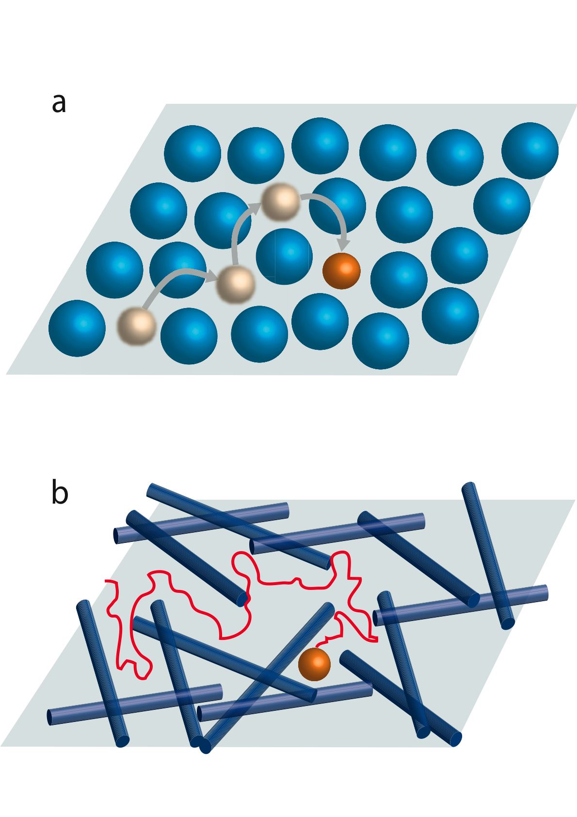
Figure 1:

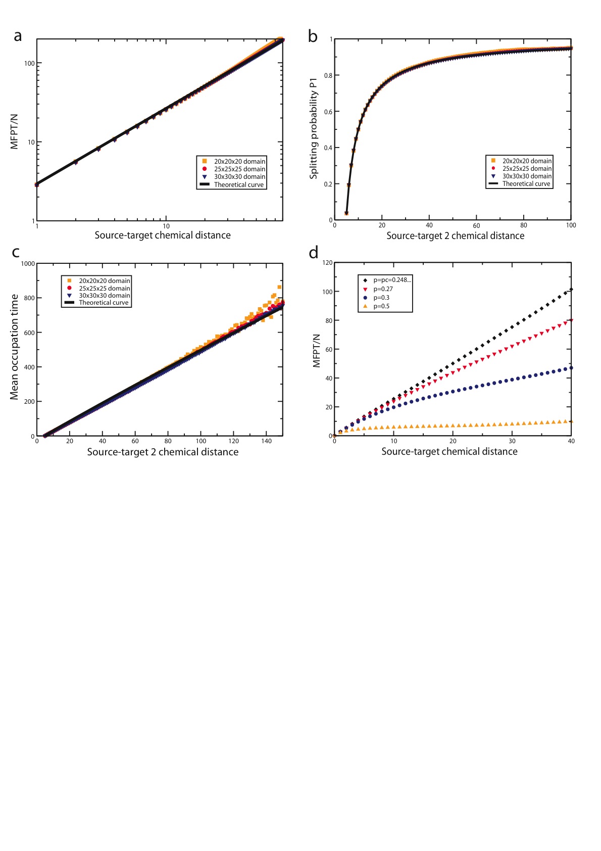
Figure 2:

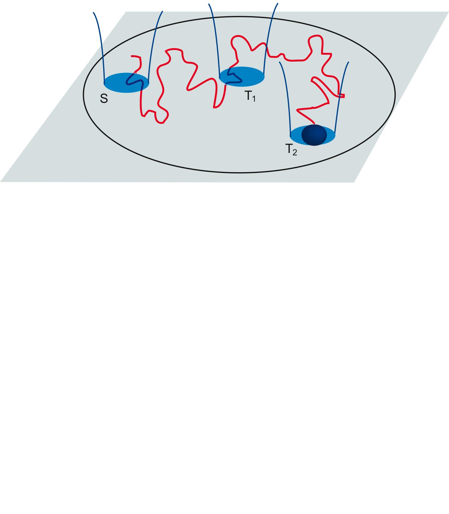
Figure 3:

References

- (1) R.Metzler and J.Klafter (2000) The random walk’s guide to anomalous diffusion: a fractionnal dynamics approach. Phys. Rep., 339, 1–77.
- (2) R.Metzler and J.Klafter (2004) The restaurant at the end of the random walk: recent developments in the description of anomalous transport by fractional dynamics. J.Phys.A, 37, R161–R208.
- (3) Scher, H. and Montroll, E. W. (1975) Anomalous transit-time dispersion in amorphous solids. Phys. Rev. B, 12, 2455–2477.
- (4) Kopelman, R., Klymko, P. W., Newhouse, J. S., and Anacker, L. W. (1984) Reaction kinetics on fractals: Random-walker simulations and excition experiments. Phys. Rev. B, 29, 3747–3748.
- (5) Scher, H., Margolin, G., Metzler, R., Klafter, J., and Berkowitz, B. (2002) The dynamical foundation of fractal stream chemistry: The origin of extremely long retention times. Geophys.Res.Lett., 29, 1061.
- (6) Tolic-Norrelykke, I. M., Munteanu, E. L., Thon, G., Oddershede, L., and Berg-Sorensen, K. (2004) Anomalous diffusion in living yeast cells. Physical Review Letters, 93, 078102.
- (7) Golding, E. and Cox, E. (2006) Physical nature of bacterial cytoplasm. Phys. Rev. Lett., 96, 981102.
- (8) Caspi, A., Granek, R., and Elbaum, M. (2000) Enhanced diffusion in active intracellular transport. Physical Review Letters, 85, 5655–5658.
- (9) Yamada, S., Wirtz, D., and Kuo, S. C. (2000) Mechanics of living cells measured by laser tracking microrheology. Biophysical Journal, 78, 1736–1747.
- (10) Wachsmuth, M., Waldeck, W., and Langowski, J. (2000) Anomalous diffusion of fluorescent probes inside living cell nuclei investigated by spatially-resolved fluorescence correlation spectroscopy. Journal Of Molecular Biology, 298, 677–689.
- (11) Platani, M., Goldberg, I., Lamond, A. I., and Swedlow, J. R. (2002) Cajal body dynamics and association with chromatin are atp-dependent. Nature Cell Biology, 4, 502–508.
- (12) Kusumi, A., Sako, Y., and Yamamoto, M. (1993) Confined lateral diffusion of membrane-receptors as studied by single-particle tracking (nanovid microscopy) - effects of calcium-induced differentiation in cultured epithelial-cells. Biophysical Journal, 65, 2021–2040.
- (13) Ghosh, R. N. and Webb, W. W. (1994) Automated detection and tracking of individual and clustered cell-surface low-density-lipoprotein receptor molecules. Biophysical Journal, 66, 1301–1318.
- (14) Smith, P. R., Morrison, I. E. G., Wilson, K. M., Fernandez, N., and Cherry, R. J. (1999) Anomalous diffusion of major histocompatibility complex class i molecules on hela cells determined by single particle tracking. Biophysical Journal, 76, 3331–3344.
- (15) Amblard, F., Maggs, A. C., Yurke, B., Pargellis, A. N., and Leibler, S. (1996) Subdiffusion and anomalous local viscoelasticity in actin networks. Physical Review Letters, 77, 4470–4473.
- (16) Le Goff, L., Hallatschek, O., Frey, E., and Amblard, F. (2002) Tracer studies on f-actin fluctuations. Phys. Rev. Lett., 89, 258101.
- (17) Wong, I. Y., Gardel, M. L., Reichman, D. R., Weeks, E. R., Valentine, M. T., Bausch, A. R., and Weitz, D. A. (2004) Anomalous diffusion probes microstructure dynamics of entangled f-actin networks. Phys. Rev. Lett., 92, 178101–4.
- (18) Banks, D. S. and Fradin, C. (2005) Anomalous diffusion of proteins due to molecular crowding. Biophysical Journal, 89, 2960–2971.
- (19) J.Klafter, A.Blumen, and M.F.Shlesinger (1987) Stochastic pathway to anomalous diffusion. Phys.Rev.A, 35, 3081–3085.
- (20) W.R.Schneider and W.Wyss (1987) Fractionnal diffusion and wave equations. J.Math.Pys., 30, 134–144.
- (21) Sokolov, I. and Klafter, J. (2006) Field-induced dispersion in subdiffusion. Phys. Rev. Lett., 97, 140602.
- (22) Saxton, M. J. (1996) Anomalous diffusion due to binding: A monte carlo study. Biophysical Journal, 70, 1250–1262.
- (23) Saxton, M. J. (2007) A biological interpretation of transient anomalous subdiffusion. i. qualitative model. Biophysical Journal, 92, 1178–1191.
- (24) D.Ben-Avraham and S.Havlin (2000) Diffusion and reactions in fractals and disordered systems. Cambridge University Press.
- (25) Bunde, A. and Havlin, S. (eds.) (1991) Fractals and disordered systems. Springer-Verlag, Berlin.
- (26) d’Auriac, J., A.Benoit, and A.Rammal (1983) Random walk on fractals: numerical studies in two dimensions. J.Phys.A, 16, 4039.
- (27) Saxton, M. J. (1994) Anomalous diffusion due to obstacles - a monte-carlo study. Biophysical Journal, 66, 394–401.
- (28) de Gennes, P. (1976) La percolation: un concept unificateur. La Recherche, 7, 919.
- (29) Lomholt, M. A., Zaid, I. M., and Metzler, R. (2007) Subdiffusion and weak ergodicity breaking in the presence of a reactive boundary. Physical Review Letters, 98, 200603.
- (30) Alberts, B., Johnson, A., Lewis, J., Raff, M., Roberts, K., and Walter, P. (2002) Molecular Biology of the Cell. Garland New York.
- (31) Rice, S. (1985) Diffusion-Limited Reactions. Elsevier, Amsterdam.
- (32) S.B.Yuste and K.Lindenberg (2002) Subdiffusion-limited reactions. Chem.Phys., 284, 169–180.
- (33) Loverdo, C., Bénichou, O., Moreau, M., and Voituriez, R. (2008) Enhanced reaction kinetics in biological cells. Nature Physics, 4, 134 - 137.
- (34) Slutsky, M. and Mirny, L. A. (2004). Biophys. J., 87, 1640.
- (35) Coppey, M., Bénichou, O., Voituriez, R., and Moreau, M. (2004) Kinetics of target site localization of a protein on dna: A stochastic approach. Biophys. J., 87, 1640–1649.
- (36) Bénichou, O., Coppey, M., Moreau, M., Suet, P.-H., and Voituriez, R. (2005) Optimal search strategies for hidden targets. Phys. Rev. Lett., 94, 198101–4.
- (37) Bénichou, O., Loverdo, C., Moreau, M., and Voituriez, R. (2006) Two-dimensional intermittent search processes: An alternative to lévy flight strategies. Phys. Rev. E, 74, 020102–4.
- (38) Eliazar, I., Koren, T., and Klafter, J. (2007) Searching circular dna strands. Journal Of Physics-Condensed Matter, 19, 065140.
- (39) Kolesov, G., Wunderlich, Z., Laikova, O. N., Gelfand, M. S., and Mirny, L. A. (2007) How gene order is influenced by the biophysics of transcription regulation. PNAS, 104, 13948–13953.
- (40) Condamin, S., Bénichou, O., Tejedor, V., Voituriez, R., and Klafter, J. (2007) First-passage times in complex scale invariant media. Nature, 450, 77–80.
- (41) Shlesinger, M. (2007) First encounters. Nature, 450, 40–41.
- (42) Redner, S. (2001) A guide to first passage time processes. Cambridge University Press, Cambridge, England.
- (43) Blanco, S. and Fournier, R. (2003) An invariance property of diffusive random walks. Europhys. Lett, 61, 168–173.
- (44) Bénichou, O., Coppey, M., Moreau, M., Suet, P., and R.Voituriez (2005) Averaged residence times of stochastic motions in bounded domains. Europhys. Lett., 70, 42–48.
- (45) Condamin, S., Tejedor, V., and Benichou, O. (2007) Occupation times of random walks in confined geometries: From random trap model to diffusion-limited reactions. Physical Review E, 76, 050102.
- (46) Condamin, S., Bénichou, O., and Moreau, M. (2005) First-passage times for random walks in bounded domains. Phys. Rev. Lett., 95, 260601.
- (47) Condamin, S., Bénichou, O., and Moreau, M. (2007) Random walks and brownian motion: a method of computation for first-passage times and related quantities in confined geometries. Phys.Rev.E, 75, 21111.
- (48) van Kampen, N. G. (1992) Stochastic Processes in Physics and Chemistry. North-Holland, Amsterdam.
- (49) Hughes, B. D. (1995) Random Walks and Random Environments. Oxford Science Publication.
- (50) Barton, G. (1989) Elements of Green’s Functions and Propagation. Oxford Science Publications.
- (51) Havlin, S. and ben Avraham, D. (1987) Diffusion in disordered media. Adv.in Phys., 36, 695.
- (52) Condamin, S., Bénichou, O., and Klafter, J. (2007) First passage time distributions for subdiffusion in confined geometries. Phys.Rev.Lett, 98, 250602.
- (53) Bouchaud, J.-P. and Georges, A. (1990) Anomalous diffusion in disordered media: statistical mechanisms, models and applications. Phys.Rep., 195, 127–293.
- (54) Blumen, A., Klafter, J., White, B. S., and Zumofen, G. (1984) Continuous-time random walks on fractals. Phys. Rev. Lett., 53, 1301–1305.