Novel interface-selected waves and their influences on wave competitions

Abstract

The topic of interface effects in wave propagation has attracted great attention due to their theoretical significance and practical importance. In this paper we study nonlinear oscillatory systems consisting of two media separated by an interface, and find a novel phenomenon: interface can select a type of waves (ISWs). Under certain well defined parameter condition, these waves propagate in two different media with same frequency and same wave number; the interface of two media is transparent to these waves. The frequency and wave number of these interface-selected waves (ISWs) are predicted explicitly. Varying parameters from this parameter set, the wave numbers of two domains become different, and the difference increases from zero continuously as the distance between the given parameters and this parameter set increases from zero. It is found that ISWs can play crucial roles in practical problems of wave competitions, e.g., ISWs can suppress spirals and antispirals.

The behaviors of waves around interface between two media have attracted continual and great interest [1-7]. In linear optics we are familiar with the problems of wave reflection and refraction, which are predicted analytically. However, for nonlinear systems the interface-related behaviors become much more complex and diverse, and much less known.

The problems of wave propagation in linear and nonlinear media have also attracted considerable attention. Recently, new observations of inwardly propagating waves have stimulated considerable interest in this field. For several centuries, scientists have known waves propagating forwardly from wave source only, called normal waves (NW). In recent years, different types of waves propagating toward the wave source (called here antiwaves, AW) have been observed in both linear optics [1, 8] and nonlinear oscillatory systems [9-14]. These new phenomena introduce completely new topics of the interface problem. For instance, novel phenomenon of negative refraction has been reported in both linear optics [1, 8] and nonlinear oscillatory systems [3,7].

In the present paper, we find another completely new nonlinear interface-phenomenon: interface of two different media can generate waves, called here interface selected waves (ISWs). In a well defined parameter surface the frequency and wave number (also wave length) of ISWs are identical in two media with different parameters, and they can be predicted analytically. Away but near this surface ISWs still exist, though the above analytical predictions are no longer available and wave numbers of ISWs in the two domains are no longer identical. By varying parameter away from this surface continuously, wave numbers change continuously, and the difference of wave numbers in two domains also increases from zero continuously. It is found that ISWs play crucial roles in practical problems of wave competitions in oscillatory systems, e.g., in suppressing spirals and antispirals.

We consider the following bidomain reaction-diffusion system

$$\frac{\partial\mathbf{U}_{1}}{\partial t} =\mathbf{f}(\mathbf{U}_{1},\bm{\mu}_{1},\bm{\nu}_{1})+\mathbf{D}(\bm{\gamma}_{1}):\nabla^{2}\mathbf{U}_{1}$$ (1a)

$$\frac{\partial\mathbf{U}_{2}}{\partial t} =\mathbf{f}(\mathbf{U}_{2},\bm{\mu}_{2},\bm{\nu}_{2})+\mathbf{D}(\bm{\gamma}_{2}):\nabla^{2}\mathbf{U}_{2}$$ (1b)

$$\mathbf{U}_{i}=(U_{i}^{(1)} ,\cdots,U_{i}^{(m)}),\quad\bm{\mu}_{i}=(\mu_{i}^{(1)},\cdots,\mu_{i}^{(p)}),$$

$$\bm{\nu}_{i}=(\nu_{i}^{(1)} ,\cdots,\nu_{i}^{(q)}),\quad\bm{\gamma}_{i}=(\gamma_{i}^{(1)};\cdots,\gamma_{i}^{(l)}),$$

$$i=1,2,\ \ m\geq 2$$

where $\mathbf{D}(\bm{\gamma}_{i})$ is a $m\times m$ matrix with constant elements depending on $\bm{\gamma}_{i}$. The function $\mathbf{f}$ and diffusion matrix $\mathbf{D}$ in the two domains are identical because the same reaction-diffusion processes occur in both sides. On the other hand, the dynamical evolutions in each side may be different due to different control parameters $(\bm{\mu}_{1},\ \bm{\nu}_{1},\ \bm{\gamma}_{1})$ and $(\bm{\mu}_{2},\ \bm{\nu}_{2},\ \bm{\gamma}_{2})$. We represent the interface between the two domains by $I$, then the following boundary conditions are required on $I$

$$\mathbf{U}_{1\{I\}}=\mathbf{U}_{2\{I\}},\ \frac{\partial\mathbf{U}_{1}}{\partial n_{\{I\}}}=\frac{\partial\mathbf{U}_{2}}{\partial n_{\{I\}}}$$ (2)

where $\frac{\partial\mathbf{U}_{i}}{\partial n_{\{I\}}}$ indicates a derivative of $\mathbf{U}_{i}$ over space variable along the direction perpendicular to the interface $I$. We assume that $\mathbf{U}_{1}=\mathbf{U}_{2}=0$ is a stable point of Eq.(1) and $\bm{\mu}_{i}(\bm{\nu}_{i})$ controls (not controls) the linear terms of $\mathbf{U}_{i}$ for the reaction parts. Hopf bifurcation with frequency $\omega_{0}$ is supposed to occur at parameters $\bm{\mu}_{1}=\bm{\mu}_{2}=\bm{\mu}_{0}$. Moreover, we assume further that both $\bm{\mu}_{1}$ and $\bm{\mu}_{2}$ are slightly beyond the Hopf bifurcation point

$$\sum_{j=1}^{p}({\mu_{i}}^{(j)}-{\mu_{0}}^{(j)})^{2}\ll 1,\ i=1,2$$ (3)

At $\bm{\mu}_{i}$, $\mathbf{U}_{i}$ performs periodic oscillation of frequency $\omega_{i}$, and $\omega_{i}$ approaches to $\omega_{0}$ as $\bm{\mu}_{i}$ reduces to $\bm{\mu}_{0}$ ($i=1,\ 2$). Under condition(3) Eq.(1) can be reduced to amplitude equations, i.e., the bidomain complex Ginzburg-Landau equations (BCGLE) by the approach standard for the derivative of single-domain CGLE [15, 16].

$$\frac{\partial A_{1}}{\partial t}=a_{1}(1-i\Omega_{1})A_{1}-b_{1}(1+i\alpha_{1})|A_{1}|^{2}A_{1}+c_{1}(1+i\beta_{1})\nabla^{2}A_{1}$$ (4a)

$$\frac{\partial A_{2}}{\partial t}=a_{2}(1-i\Omega_{2})A_{2}-b_{2}(1+i\alpha_{2})|A_{2}|^{2}A_{2}+c_{2}(1+i\beta_{2})\nabla^{2}A_{2}$$ (4b)

$$A_{1\{I\}}=A_{2\{I\}},\ \frac{\partial A_{1}}{\partial n_{\{I\}}}=\frac{\partial A_{2}}{\partial n_{\{I\}}}$$ (4c)

where $(a_{i},\ \Omega_{i})$, $(b_{i},\ \alpha_{i})$ and $(c_{i},\ \beta_{i})$ are related to $\bm{\mu}_{i}-\bm{\mu}_{0}$, $(\bm{\mu}_{i}-\bm{\mu}_{0},\ \bm{\nu}_{i})$ and $(\bm{\mu}_{i}-\bm{\mu}_{0},\ \bm{\gamma}_{i})$, respectively. The continuity conditions Eq.(4c) can be derived from condition (2) because the transformation from $U_{1}$ to $A_{1}$ is exactly the same as that from $U_{2}$ to $A_{2}$ (in the two domains, amplitude equations are derived at a common Hopf bifurcation point with an identical linear matrix at $\bm{\mu}_{0}$), and the transformations from $U_{i}$ to $A_{i}$ ($i=1,2$) are determined only by this linear matrix. In Eq.(4) $A_{1}$ and $A_{2}$ are complex variables in each side of the interface. With scaling transformations we can fix $a_{1},\ b_{1},\ c_{1}$ and $\Omega_{1}$, and the remaining 8 parameters are irreducible for BCGLE systems. In the following study we will set $a_{1}=b_{1}=c_{1}=1,\ \Omega_{1}=0$ for numerical simulations without mentioning and all the theoretical formulas are given generally for 12 parameters. Without the interface interaction, the two media have their single-domain planar wave solutions [2, 17]

$$A_{i}(x,t)=\sqrt{(\frac{1}{b_{i}}(a_{i}-c_{i}k_{i}^{2}))}e^{i(k_{i}x-\omega_{i}t)},\ 0\leq k^{2}_{i}\leq\frac{a_{i}}{c_{i}}$$ (5a)

$$\omega_{i}=a_{i}(\alpha_{i}+\Omega_{i})+c_{i}(\beta_{i}-\alpha_{i})k^{2},\ a_{i},b_{i},c_{i}>0$$ (5b)

Waves in media $M_{1}$ and $M_{2}$ are classified to NWs and AWs under the conditions [3, 12, 14]

$$NWs:\ \omega_{i}a_{i}(\Omega_{i}+\alpha_{i})<0\ ;\ or,\ \omega_{i}a_{i}(\Omega_{i}+\alpha_{i})>0\ and\ |\omega_{i}|>|a_{i}(\Omega_{i}+\alpha_{i})|$$ (6a)

$$AWs:\ \omega_{i}a_{i}(\Omega_{i}+\alpha_{i})>0\ and\ |\omega_{i}|<|a_{i}(\Omega_{i}+\alpha_{i})|$$ (6b)

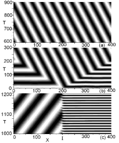
Figure 1: (a)-(c) Contour patterns of Re$A_{i}$ of a 1D BCGLE system with interface $I$. Domains $M_{i},\ (i=1,2)$ have length $L$ and parameters $\alpha_{i},\ \beta_{i}$, and $a_{i}=b_{i}=c_{i}=1,\ \Omega_{i}=0,\ i=1,2$. Numerical simulations are made with space step $dx=0.5$, time step $dt=0.005$, and $L=200$. No-flux boundary condition, randomly chosen initial conditions and the above time and space steps are used in all figures for numerical simulations unless specified otherwise. (a) $\alpha_{1}=0.1,\ \beta_{1}=-1.4,\ \alpha_{2}=-0.2,\ \beta_{2}=1.4$. Interface-selected waves (ISWs) homogeneous in $M_{1}$ and $M_{2}$ are observed, and the interface is transparent to ISWs. (b) The same as (a) with early time evolution plotted. It is clearly shown that ISWs originate from the interface. (c) $\alpha_{1}=0.1,\ \beta_{1}=-1.4,\ \alpha_{2}=0.5,\ \beta_{2}=1.4$. $M_{1}$ and $M_{2}$ support different regular waves, clearly manifesting interface $I$.

By AWs we mean waves with negative phase velocity, while both NWs and AWs have positive group velocities [11, 12, 14]. Now we focus on the interface related problems, and start from a one-dimensional (1D) BCGLE system. We are interested in the problem how the interface can significantly influence the system dynamics. In Fig.1(a)-(c) we study the system evolutions at two different parameter sets with random initial conditions, and find characteristically different features in the asymptotic states. The most significant and new observation is given in Figs.1(a) and 1(b) where we find homogeneous planar waves moving in both media from right to left with a constant velocity and transparently crossing the interface. These homogeneous running waves originate from the interface (see Fig.1(b)), therefore, called interface selected waves (ISWs). The phenomenon of Fig.1(a) is surprising. With two media having different control parameters we intuitively expect that the waves in two media must have different wave numbers (even if both sides may have the same frequency). This common feature is clearly seen in Fig.1(c) where we observe uniform bulk oscillation in the right medium and waves propagating from left to right in the left medium, clearly manifesting the interface $I$. However, in Fig.1(a) waves propagate seemly in a homogeneous medium without feeling any difference of $M_{1}$ and $M_{2}$; the interface is transparent to the waves. Moreover, the realization of these running waves is stable against different initial perturbations. This characteristic phenomenon can never exist in linear systems, and has never been observed so far in nonlinear systems.

It is interesting that we can predict the frequency and wave number of ISWs explicitly and exactly under certain parameter conditions. For case of Fig.1(a) we can determine the frequency and wave number by the following simple requirements:

$$\omega_{1}(k_{1})=\omega_{2}(k_{2}),\ k_{1}=k_{2},\ |A_{1}|=|A_{2}|$$ (7)

Inserting Eqs.(7) into Eq.(5) we obtain a unique set of solutions $\omega_{I},k_{I}$

$$k_{1}^{2}=k_{2}^{2}=k_{I}^{2}=\frac{a_{1}(\alpha_{1}+\Omega_{1})-a_{2}(\alpha_{2}+\Omega_{2})}{c_{2}(\beta_{2}-\alpha_{2})-c_{1}(\beta_{1}-\alpha_{1})}$$ (8a)

$$\omega_{1}=\omega_{2}=\omega_{I}=\frac{a_{1}(\alpha_{1}+\Omega_{1})c_{2}(\beta_{2}-\alpha_{2})-c_{1}(\beta_{1}-\alpha_{1})a_{2}(\alpha_{2}+\Omega_{2})}{c_{2}(\beta_{2}-\alpha_{2})-c_{1}(\beta_{1}-\alpha_{1})}$$ (8b)

And these solutions are exact in the parameter surface

$$for\ c_{1}b_{2}-c_{2}b_{1}\neq 0:\ if\ and\ only\ if\ \frac{a_{1}b_{2}-a_{2}b_{1}}{c_{1}b_{2}-c_{2}b_{1}}-\frac{a_{1}(\alpha_{1}+\Omega_{1})-a_{2}(\alpha_{2}+\Omega_{2})}{c_{2}(\beta_{2}-\alpha_{2})-c_{1}(\beta_{1}-\alpha_{1})}=0$$ (8c)

$$for\ c_{1}b_{2}-c_{2}b_{1}=0:\ if\ and\ only\ if\ a_{1}b_{2}-a_{2}b_{1}=0$$

which is obtained by inserting Eq.(8a) into Eq.(5a), and by the identifying $|A_{1}|=|A_{2}|$. It can be easily confirmed that on the parameter surface Eq.(8c) the planar wave solution Eq.(5) with frequency and wave numbers given by Eqs.(8a) and (8b) are exact solution of BCGLE. Moreover, the predictions of Eqs.(7) and (8) agree exactly with the numerical results of Fig.1(a).

In Figs.2(a) and 2(b) we specify the surface of Eq.(8c) in some parameter planes where solid lines represent the parameters satisfying condition (8c). In Figs.2(c) and 2(d) we vary parameters along the solid line of Fig.2(a) and numerically compute 1D BCGLE. we compare the numerical results (empty cycles and triangles) with theoretical predictions of Eqs.(8a) and (8c) (solid lines), and find: (i) ISWs exist in a large area of surface Eq.(8c); (ii) the predictions of Eqs.(8a) and (8b) coincide with numerical results exactly (within computation precision). In Fig.2(e) we fix a parameter set on the surface (black disk T) and present the asymptotic pattern evolution of the BCGLE system. It is clearly shown that ISWs, with the wave number and frequency predicted by Eqs.(8a) and (8b), asymptotically control the entire bidomain during their propagation. For demonstrating the possibility of observation of ISWs in experiments, we study a reaction-diffusion model: bidomain Brusselator. In Fig.2(f), we show ISWs of this chemical model, satisfying all conditions of Eqs.(7).

The solutions of Eqs.(8a) and (8b) are exact for BCGLE only on the parameter surface of Eq.(8c). Slightly away from this surface Eqs.(8a) and (8b) can no longer predict the wave numbers and the frequencies of ISWs exactly. In Figs.3(a) and 3(b) we compare the theoretical predictions of Eqs.(8a) and (8b) with numerical results of frequencies and wave numbers by varying parameters along the dashed line in Fig.2(a). We find: (i) The solutions of Eqs.(8a) and (8b) are not exact; the wave numbers in the two domains deviate from each other (about $7.7\%$ difference in Fig.3(d)); (ii) However, slightly away from the surface Eq.(8c), the feature that the interface generates waves is still clearly observed (compare Fig.1(b) with Fig.3(c)), i.e., ISWs still exist; (iii) By continuously increasing the parameter distance from condition Eq.(8c), the deviation of the numerical results from the theoretical predictions Eqs.(8a) and (8b) increases continuously from zero too, and for small parameter deviation the solutions Eqs.(8a) and (8b) can still be used for predicting frequency and wave numbers with very good approximation. In Figs.3(c) and 3(d) we show ISWs for a parameter set away from the surface Eq.(8c) (Disk Q in Fig.2(a)). It is clear that even away from surface Eq.(8c) the waves of Fig.3(c) are generated by the interface in the similar way as in Fig.1(b) though we have $k_{1}=k_{2}$ in Fig.1(b) but $k_{1}\neq k_{2}$ in Fig.3(c). Thus the waves in Fig.1(a), 1(b) and Figs.3(c), 3(d), have obviously the same interface-selected nature which is essentially different from the waves of Fig.1(c). Similar ISWs with $k_{1}\neq k_{2}$ can also be observed in bidomain Brusselator. In Figs.3(e) and 3(f) we take parameter set far away from that in Fig.2(f), and can still observe ISWs. Here the wave numbers in the two sides have slight difference ($\frac{2|k_{1}-k_{2}|}{|k_{1}+k_{2}|}\approx 6.77\%$).

There are some necessary conditions for ISWs to appear. Let us analytically specify some of these conditions under Eq.(8c) (Eqs.(8a) and (8b) are exact solutions of $\omega_{I}$ and $k_{I}$). From Eqs.(8a) and (5a) we have an obvious necessary existence condition for ISWs, i.e.,

$$0\leq k_{I}^{2}=\frac{a_{1}(\alpha_{1}+\Omega_{1})-a_{2}(\alpha_{2}+\Omega_{2})}{c_{2}(\beta_{2}-\alpha_{2})-c_{1}(\beta_{1}-\alpha_{1})}\leq\frac{a_{i}}{c_{i}},\ i=1,2$$ (9a)

which should be satisfied because wave number $$k_{I} k_{I} \omega_{I}$$ must be real. If this condition is violated, there is no physically meaningful solutions of and , and thus no ISWs can be observed. This is the case of Fig.1(c). ISWs are generated by the interface and propagate along a certain direction. Therefore, the waves must forwardly propagate in one domain. Precisely, ISWs are NWs in the left (or right) domain while AWs in the right (left) domain for waves propagating from right (left) to left (right), and this requires another parameter condition

$$AWs:\ \omega_{I}a_{i}(\Omega_{i}+\alpha_{i})>0\ and\ |\omega_{I}|<|a_{i}(\Omega_{i}+\alpha_{i})|\$$ (9b)

$$NWs:\ \omega_{I}a_{\bar{i}}(\Omega_{\bar{i}}+\alpha_{\bar{i}})<0\ or\ \omega_{I}a_{\bar{i}}(\Omega_{\bar{i}}+\alpha_{\bar{i}})>0\ and\ |\omega_{I}|>|a_{\bar{i}}(\Omega_{\bar{i}}+\alpha_{\bar{i}})|\$$

$$i=1,\ \bar{i}=2\ or\ i=2,\ \bar{i}=1$$

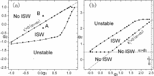
Figure 4: The distributions of different types of waves in ($\alpha_{1},\ \alpha_{2}$) parameter planes for different sets of ($\beta_{1},\ \beta_{2}$). Black disks represent the boundaries of ISW regions (”ISW” regions) identified by direct numerical simulations of 1D BCGLE. In ”No ISW” regions, ISWs do not exist due to the violations of condition Eq.(9a) (boundary $k^{2}_{I}=0$, i.e., $\alpha_{1}=\alpha_{2}$) or condition Eq.(9b) (boundary $\alpha_{i}=\beta_{i},\ i=1$ or $2$) (both presented in dashed-dotted lines). In the region ”Unstable”, both conditions Eqs.(9a) and (9b) are satisfied, but waves with the given $k_{I}$ are unstable due to the Eckhaus instability. $a_{i}=b_{i}=c_{i}=1,\ \Omega_{i}=0,\ i=1,2.$ (a) $\beta_{1}=-1.4,\beta_{2}=1.4$, (b) $\beta_{1}=2.5,\beta_{2}=0.5$. Black triangles A and B in Fig.4(a) represent the parameter sets used in Figs.1(a), (c), respectively.

In order to provide an idea how these conditions influence the existence of ISWs, we show Fig.4, where one can numerically observe ISWs in the regions enclosed by disks, called ”ISW” regions. In Fig.4 dashed-dotted lines with $k^{2}_{I}=0$ and $\alpha_{i}=\beta_{i},\ i=1\ or\ 2$ are the boundaries of ”ISW” theoretically predicted by Eqs.(9a)and (9b), respectively. In ”No ISW” regions ISWs do not exist due to violations of conditions of Eq.(9a) or (9b). In the regions ”Unstable”, ISWs exist while waves with wave number $k_{I}$ are unstable due to Eckhaus instability, and there ISWs cannot be numerically observed. Figures 4(a) and 4(b) are plotted in a small parameter surface under the condition of Eq.(8c). Similar structure of distributions ”ISW”, ”No ISW” and ”Unstable” regions can be observed when parameters are varied slightly away from the set of Eq.(8c).

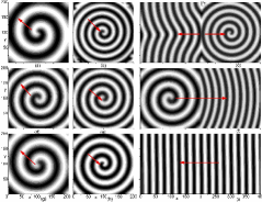
Figure 5: Wave competitions between spiral, antispiral and ISWs in 2D BCGLE with interface $II^{\prime}$. $a_{i}=b_{i}=c_{i}=1,\ \Omega_{i}=0,\ i=1,2$. (a)(d)(g) Spirals in $M_{1}$ medium. (b)(e)(h) Antispirals in $M_{2}$ medium. Snapshots in (a)(b), (d)(e) and (g)(h) are used as the initial conditions for the dynamic evolutions of (c), (f) and (i), respectively. (c)(f)(i) The asymptotic states of bidomain systems with interface $II^{\prime}$. (a)(b)(c) $\alpha_{1}=0.2,\ \beta_{1}=2.0,\ \alpha_{2}=1.0,\ \beta_{2}=-0.5$. Antispiral initially in $M_{2}$ dominates the system in (c). (d)(e)(f) $\alpha_{1}=0.2,\ \beta_{1}=-2.0,\ \alpha_{2}=0.5,\ \beta_{2}=-1.4$. Spiral initially in $M_{1}$ dominates the system in (f). (g)(h)(i) $\alpha_{1}=0.1,\ \beta_{1}=3.2,\ \alpha_{2}=1.2,\ \beta_{2}=0.0$. In (i) ISWs suppress both spiral in $M_{1}$ and antispiral in $M_{2}$, and dominate the whole system.

Though the above investigations are made for 1D bidomain systems, the observations of ISWs exist generally for high-dimensional systems. In 2D oscillatory systems, much richer types of waves, including spirals and antispirals, can be self-sustained, and wave competitions become an important issue. Now we explore how ISWs play crucial roles in wave competitions. We consider a 2D BCGLE system with an interface line $II^{\prime}$ in between. Without the interface interaction, $M_{1}$ supports normal spirals (Figs.5(a), (d), (g)) and $M_{2}$ supports antispirals ( Figs.5(b), (e), (h)). With the interface interaction we find characteristically different results of wave competitions. Fig.5(c): the antispiral wins the competition and dominates the system with frequency $\omega_{2}$; Fig.5(f): the spiral wins; Fig.5(i): ISWs win and dominate the two domains. The reasons why we can observe so diverse results in similar competitions between spiral and antispiral waves can be completely understood based on the analysis of ISWs.

For explaining the results of Fig.5 we briefly introduce some known conclusions on wave competitions in oscillatory systems. If competitions occur in a homogeneous medium, the results are [3, 18]:

$$NWs\ against\ NWs:\ faster\ waves\ win$$ (10a)

$$AWs\ against\ AWs:\ slower\ waves\ win$$ (10b)

$$NWs\ against\ AWs:\ NWs\ win$$ (10c)

With the competition rules Eq.(10) and the analytical results of Eqs.(7)-(9) we can fully understand and predict the diverse results of Fig.5.

Inserting the parameters of Fig.5(c) into Eq.(8) we have $\omega_{I}=0.636$. Considering conditions Eq.(6) we conclude that ISWs are NWs in $M_{1}$ and AWs in $M_{2}$ (note, the interface is the source of ISWs). The frequencies of the spiral in $M_{1}$ and the antispiral in $M_{2}$ are $\omega_{1}=0.288$ and $\omega_{2}=0.626$, respectively. According to conclusion (10) ISWs win the competition in $M_{1}$ against the spiral while losing the battle in $M_{2}$ against the AW spiral. Therefore, the antispiral waves of frequency $\omega_{2}$ finally dominate the whole system. The parameters of Fig.5(f) do not satisfy condition Eq.(9a), and no ISWs can be generated. In Figs.5(d) and (e) we observe $\omega_{1}=-0.0567$ and $\omega_{2}=0.151$. According to Eq.(6) waves of $\omega_{1}(\omega_{2})$ are NWs (AWs) in both $M_{1}$ and $M_{2}$. On the basis of (10c), the spiral of frequency $\omega_{1}$ wins the competition. The most interesting observation is given in Fig.5(i) where we have $\omega_{I}=0.932$. The frequency of the spiral(antispiral) in $M_{1}$ ($M_{2}$) is $\omega_{1}=0.293$ ($\omega_{2}=1.037$). Therefore, ISWs win both competitions against the spiral in $M_{1}$ (condition (10a)) and against the antispiral in $M_{2}$ (condition (10b)). The asymptotic state is ISWs in 2D system where ISWs suppress both spiral and antispiral in Fig.5(i).

In conclusion, we investigated the role played by interfaces. A new type of waves, interface selected waves (ISWs) were found in bidomain systems with one medium supports AWs and the other NWs. When control parameters are on a well defined parameter surface ISWs propagate with analytically predictable same frequency and wave number in two media with different parameters. When the parameters are away but near this surface, ISWs can be also observed, of which the frequency and wave numbers can be located approximately. These waves are selected by interfaces between two media, and some necessary conditions for observing these ISWs are specified. These ISWs play important roles in wave competitions. For instance, under certain conditions ISWs can suppress spiral and antispiral waves in both media. These roles are important in practical applications. Experimental realizations of ISWs in chemical reaction-diffusion systems are strongly suggested, based on the well-behaved ISWs of Fig.2(f), Fig.3(e) and Fig.3(f) computed for a chemical reaction-diffusion model.

1. R. A. Shelby, D. R. Smith, and S. Schultz, Science 292, 77 (2001).
2. M. Hendrey, E. Ott, and T. M. Antonsen Jr., Phys. Rev. Lett. 82, 859 (1999); Phys. Rev. E 61, 4943 (2000).
3. Z. Cao, H. Zhang, and G. Hu, Eur. Phys. Lett. 79, 34022(2007).
4. M. Vinson, Physica D 116, 313 (1998).
5. M. Zhan, X. Wang, X. Gong, and C. H. Lai, Phys. Rev. E 71, 036212 (2005).
6. L. B. Smolka, B. Marts, and A. L. Lin, Phys. Rev. E 72, 056205 (2005).
7. R. Zhang, L. Yang, A. M. Zhabotinsky, and I. R. Epstein, Phys. Rev. E 76, 016201 (2007);
8. C. G. Parazzoli, D. B. Brock, and S. Schultz, Phys. Rev. Lett. 90, 107401 (2003).
9. V. K. Vanag and I. R. Epstein, Science 294, 835 (2001); Phys. Rev. Lett. 88, 088303 (2002).
10. L. Yang, M. Dolnik, A. M. Zhabotinsky, and I. R. Epstein, J. Chem. Phys. 117, 7259 (2002).
11. Y. Gong and D. J. Christin, Phys. Rev. Lett. 90, 088302 (2003); Phys. Lett. A 331, 209 (2004).
12. L. Brusch, E. M. Nicola, and M. Bär, Phys. Rev. Lett. 92, 089801 (2004); E. M. Nicola, L.Brusch, and M. Bär, J. Phys. Chem. B 108 14733 (2004).
13. P. Kim, T. Ko, H. Jeong, and H. Moon, Phys. Rev. E 70, R065201 (2004).
14. Z. Cao, P. Li, H. Zhang, and G. Hu, the International Journal of Mordern Physics B 21, 4170 (2007).
15. M. Cross and P. Hohenberg, Rev. Mod. Phys. 65, 851 (1993).
16. I. S. Aranson and L. Kramer, Rev. Mod. Phys. 74, 99 (2002).
17. I. S. Aranson, and L. Aranson, Phys. Rev. A 46, R2992 (1992).
18. K. J. Lee, Phys. Rev. Lett. 79, 2907 (1997).

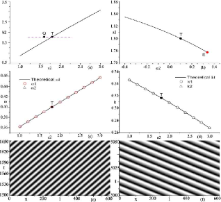
Figure 2: (a) Surface Eq.(8c) (Solid line) is plotted in $a_{2}-b_{2}$ plane with $\Omega_{2}=0,\ c_{2}=2.0,\ \alpha_{1}=0.6,\ \beta_{1}=-1.4,\ \alpha_{2}=0.1,\ \beta_{2}=1.2$. (b) The same as (a) with surface (8c) plotted in $\alpha_{2}-a_{2}$ plane, $b_{2}=1.778$. Point E corresponds to the boundary $k^{2}=0$. (c) Frequency of ISWs which are selected along the solid line of (a). Theoretical prediction Eq.(8a) (solid line) coincides with numerical simulation for 1D BCGLE (empty circles and triangles) perfectly. (d) The same as (c) with wave numbers $k_{1}=k_{2}$ plotted. Agreement between theoretical prediction Eq.(8a) and numerical results is also confirmed. (e) ISW pattern obtained by using the parameter set $a_{2}=1.8,\ b_{2}=1.778$ (point T in (a)). (f) The same as (e) with contour pattern of $v$ variable of Brusselator RD which is numerically computed for 1D chain. The system is: $\frac{\partial u_{i}}{\partial t}=a_{i}-(b_{i}+1+\gamma_{i})u+(1+\sigma_{i})u^{2}v+\delta_{ui}\nabla^{2}u,\ \frac{\partial v_{i}}{\partial t}=b_{i}u-(1+\sigma_{i})u^{2}v+\delta_{vi}\nabla^{2}v,\ i=1,2,\ a_{1}=1.0,\ b_{1}=2.24,\ \gamma_{1}=\sigma_{1}=0.0,\ \delta_{u1}=2.31,\ \delta_{v1}=2.17;\ a_{2}=1.02,\ b_{2}=2.2624,\ \gamma_{2}=0.02,\ \sigma_{2}=0.01,\ \delta_{u2}=0.95,\ \delta_{v2}=2.47;\ dx=dy=0.5,\ dt=0.0025,\ L=300$. ISWs with identical $w$ and $k$ are observed.

Figure 3: (a) (b) The same as Figs.2(c) and (d), respectively, with parameters varied along the dashed line of Fig.2(a). Numerical simulations are made for 1D BCGLE. Now deviations between theoretical results of Eqs.(8a), (8b) and the numerical results are observed. Deviation increases as parameters vary away from the surface Eq.(8c). (c) (d) The same as Fig.2(e) with different time intervals plotted, respectively, in which parameters are taken away from the solid line of Fig.2(a) (point Q, $a_{2}=1.6,\ b_{2}=1.778$). Now ISWs are still observed while wave numbers in the two sides are slightly different($\frac{2|\triangle k|}{|k_{1}+k_{2}|}\approx 7.71\%,\ \triangle k=|k_{1}-k_{2}|$). (e) (f) The same as (c) and (d), respectively, with 1D Brusselator chain computed. The parameter set is considerable different from that of Fig.2(f): $a_{1}=1.0,\ b_{1}=3.2,\ \gamma_{1}=\sigma_{1}=0.0,\ \delta_{u1}=1.0,\ \delta_{v1}=0.5;\ a_{2}=1.1,\ b_{2}=3.2,\ \gamma_{2}=0.1,\ \sigma_{2}=0.0,\ \delta_{u2}=1.0,\ \delta_{v2}=2.5$. Now the wave numbers of the two sides are also slightly different ($\frac{2|\triangle k|}{|k_{1}+k_{2}|}\approx 6.77\%$).