The Spatial String Tension and Dimensional Reduction in QCD
Abstract
We calculate the spatial string tension in (2+1) flavor QCD with physical strange quark mass and almost physical light quark masses using lattices with temporal extent and . We compare our results on the spatial string tension with predictions of dimensionally reduced QCD. This suggests that also in the presence of light dynamical quarks dimensional reduction works well down to temperatures .
pacs:
11.15.Ha, 12.38.GcI Introduction
At high temperature, strongly interacting matter undergoes a transition from a confining, chiral symmetry broken phase to a phase which is chirally symmetric and deconfining in nature. For pure gluonic matter as well as for QCD with massless quarks this transition is known to be a genuine phase transition, while for QCD with physical quark masses it is most likely only a smooth (though rapid) crossover milc04 ; fodor ; tc06 . In both cases, thermodynamic observables like energy and entropy density show a sharp increase at the transition point, but approach the expected behavior of an asymptotically free quark-gluon gas only at very high temperatures.
The phase just above is more complicated than a weakly interacting gas of quarks and gluons. Non-perturbative features like the (Debye) screening of electric modes as well as the possible appearance of a mass gap in the magnetic sector give rise to well-known problems that make a straightforward perturbative analysis of the high temperature phase of QCD fail. While infrared divergences arising at a momentum scale can still be taken into account by resummation Zhai ; Arnold ; spt97 ; Blaizot ; Andersen , the softer modes at scale reflect genuine non-perturbative physics and cannot be handled by any resummation linde .
The non-perturbative physics arising from the magnetic sector of QCD shows up at distances that are large on the scale of the inverse temperature, . It finds its most prominent reflection in the survival of an area law behavior for space-like Wilson loops, i.e. confinement of magnetic modes. The spatial string tension, , extracted from the area law behavior of spatial Wilson loops, has been studied early on in lattice calculations performed in the pure gauge sector of QCD detar ; polonyi . Detailed studies of the temperature dependence of in SU(2) and SU(3) gauge theories bali93 ; bielefeld ; eos showed the expected dependence on the magnetic scale and established a close relation to the string tension of a 3-dimensional gauge theory. A recent detailed comparison of , calculated in lattice regularized QCD, with calculations performed in the framework of dimensionally reduced QCD mikko was extremely successful in describing the temperature dependence of quantitatively even at temperatures close to the transition temperature.
Dimensional reduction makes very specific predictions for modifications induced in the magnetic sector of QCD through the presence of fermion degrees of freedom, quarks. In fact, modifications are expected to be small and the dominant structure of e.g. the spatial string tension is still expected to be controlled by a purely gluonic, 3-dimensional SU(3) gauge theory. A possible source for failure has, however, been discussed in the past gavai ; dynamical quarks, more precisely quark anti-quark pairs, can give rise to additional light bosonic quasi-particle modes that are not described by a 3-dimensional gauge theory. This makes it interesting to check to what extent dimensional reduction also is capable of describing physics in the magnetic sector of QCD in the presence of light dynamical quarks.
In this paper we calculate the spatial string tension in QCD with light dynamical quarks. For the first time we cover in such an analysis a large temperature range and perform calculations at three values of the lattice cut-off. We will present a detailed comparison of the lattice calculations with predictions based on dimensional reduction. Some preliminary results of this work have been presented in frithjof .
This paper is organized as follows. In the next section we give a brief discussion of the concepts of dimensional reduction as far as they are relevant for this work and the analysis of the spatial string tension. In Section III we present details of our calculation of spatial pseudo-potentials and in Section IV we discuss the determination of the spatial string from them. A comparison of these results with dimensional reduction is given in Section V. Finally we give our conclusions in Section VI.
II Dimensional reduction
The different non-perturbative length scales of and , respectively, that one encounters in the perturbative analysis of QCD at high temperature are convenient for the reformulation of QCD in terms of a hierarchy of effective field theories that clearly separate the physics at these different scales rob . This allows the disentanglement of sectors that can be treated in perturbation theory from sectors that are only accessible to non-perturbative techniques.
Since the partition function of an equilibrium field theory can be written as an Euclidean field theory with the time direction being a torus of extent , the temporal modes of fields are proportional to the Matsubara frequencies, , where is an integer for bosonic and a half-integer for fermionic fields. At large temperatures, therefore, the non-static bosonic fields and the fermionic fields become very heavy and can be integrated out to get an effective theory for distance scales111Distances are naturally measured in units of , and is a natural unit since the average spatial separation of partons in the high temperature phase is . which involves the static modes only rob . This gives an effective 3-dimensional theory222In this normalization convention the spatial gauge fields have dimension one, while the electric field has a dimension .,
| (1) | |||||
with the static mode of the temporal component of the gauge field, , appearing as an adjoint scalar field. The parameters of this effective theory can be calculated in perturbation theory to any order braaten95 ; kajantie97 . At leading order one has and for massless quark flavors. The deconfined phase of high temperature QCD corresponds to the symmetric (confining) phase of the above 3d adjoint Higgs theory (see discussion in kajantie97 ; karsch98 ). The confining nature of this theory is the origin of the infrared problem of high temperature QCD for momenta . At very high temperatures also the Debye mass will be large, , and the heavy field can thus also be integrated out. Therefore, for physics of distance scales , the fields can be integrated out which leads to a pure three-dimensional gauge theory,
| (2) |
The gauge coupling can be calculated in terms of and . This has been done to 2-loop accuracy giovannangeli . At leading order . The hierarchy of effective theories is referred to as the dimensional reduction scheme. The use of the dimensional reduction scheme in combination with lattice calculations performed within the effective 3-dimensional theory allows the treatment of the infrared problem of perturbative QCD at high temperature and the consistent extension of the weak coupling expansion of thermodynamic quantities to higher orders, for instance the contribution to the thermodynamic potential ( pressure ) of QCD kajantie03 .
In pure SU(N) gauge theory, the underlying nonperturbative structure of the high temperature theory can directly be seen in calculations of spatial Wilson loops. The static energy in the finite temperature theory is given by Wilson loops in space-time planes, , which are expected to satisfy a perimeter law above , thus signaling deconfinement. In contrast, entirely space-like Wilson loops, which are restricted to fixed time hyperplanes, show an area law, as they can be mapped to the energy in the confining 3-dimensional theory detar ; polonyi as indicated above. Detailed studies of spatial Wilson loops in SU(2) and SU(3) gauge theories have corroborated the dimensional reduction picture bali93 ; bielefeld ; eos . The spatial string tension , the coefficient of the area term,
| (3) |
has been found to be in very good quantitative agreement with that of the dimensionally reduced theory. Since sets the mass scale in the 3-dimensional gauge theory, one has where is a numerical factor. Dimensional reduction therefore predicts
| (4) |
to leading order, where is the temperature-dependent running coupling of the four dimensional theory and is a constant that can be determined through a non-perturbative (Monte Carlo) calculation of Wilson loops in a 3-dimensional SU(3) gauge theory bielefeld ; teper . Already this tree level matching was found to be valid to a good accuracy at temperatures as low as bielefeld ; eos . This is in accordance with studies of other correlation functions in SU(2) and SU(3) gauge theories, which also show dimensional reduction to be a valid approximation already at temperatures . It is worth mentioning that the perturbative separation of electric and magnetic scales, , is not valid at these temperatures, where and where the electric gluons thus are the lightest degrees of freedom prd ; peter ; hart . Strictly speaking, the step leading from Eq. (1) to Eq. (2) thus should not be taken. However, the Higgs sector does not seem to have a significant effect on the correlation functions of purely gluonic 3d gauge fields peter ; hart .
The situation may be somewhat different in QCD. While the quarks acquire an effective mass of , they make a qualitative difference in the long distance physics: since they provide a source for screening of fundamental charge, one expects that at sufficiently large distances (spatial) string breaking takes place, which cannot be described by the effective theories or , respectively, as those do not include fundamental charges. Of course, the distance (in units of ) one needs to reach to observe this deviation increases with temperature, so it remains an important question to ask how well the (spatial) string tension of the four dimensional theory, extracted at large distances but before string breaking sets in, can be explained by the dimensionally reduced theory. In principle it is possible to write down the theory which includes also the lowest fermion Matsubara frequency vepsalainen . This version of the dimensionally reduced theory would be able to describe the string breaking as well. At distances smaller than the string breaking scale, however, and given the weak dependence of the 3d gauge fields on the dynamics of the adjoint scalar fields discussed above we would expect that the presence of fermionic modes with mass of will have very little influence on Wilson loops, and the spatial string tension extracted from them. On the other hand, from a comparison of screening masses in a theory with = 4 degenerate light flavors, Ref. gavai argued that the presence of dynamical quarks could impede dimensional reduction. Thus, the question of an effective description of spatial Wilson loops in terms of a dimensionally reduced theory at not-too-large temperatures is not settled and needs to be treated more extensively for QCD.
III Spatial potential at finite temperature
We have carried out a study of the spatial Wilson loops for QCD in the temperature interval []. In this study we fixed the strange quark mass () to its physical value, and the quarks are taken to be degenerate with mass . These light quark masses are about a factor two heavier than physical quarks, and give a pion mass of about MeV. The gauge configurations we analyze here were generated for the study of the equation of state of hot strongly interacting matter eos_paper . The gauge action uses Wilson plaquette and rectangle terms. For the fermion action the p4fat3 staggered discretization p4fat3 was used, which adds a bended three-link term to the standard staggered action, and the 1-link gauge connections are smeared with the 3-link staples. In our analysis we have used lattices with temporal extent and and aspect ratio . The lattice spacing has been set using the Sommer parameter sommer . When quoting the results in physical units the value fm has been used gray . Given the above temporal lattice sizes and the temperature interval covered in our numerical calculations, the range of lattice spacings varied from fm to fm. Further details on the generation of gauge configurations and the action used in these calculations can be found in Ref. eos_paper .
To interpret the spatial Wilson loops as the exponential of the static potential in the effective 3-dimensional theory, we use a transfer matrix formalism in the z direction: the loops are constructed as , where is the distance between the static quark and anti-quark in the xy-plane. The loops in a timeslice were constructed using the Bresenham algorithm bresenham and they were averaged over the timeslices. The static potential, for a transfer matrix acting in the z direction, is defined as creutz
| (5) |
To obtain a better signal-to-noise ratio it is important to be able to reach the asymptotic limit already for moderate values of . To achieve this, the gauge fields connecting quark and anti-quark were smeared using 3-link staples perpendicular to the direction of the gauge field. The smearing procedure has been applied iteratively. We found that for small values of the gauge coupling () 10 APE smearing steps with a smearing coefficient of 0.4 were sufficient to give the asymptotic value already at = 3. For larger we use 30 to 60 smearing steps.
The Wilson loop ratios in Eq. (5) were performed for different , and a plateau is reached by =3. To avoid any remaining contamination from higher states, the logarithm of the ratio of Wilson loops was fitted to the ansatz . The results from the direct ratio at generally agree well with the value obtained from fits. We used in our analysis estimates for the string tension coming from Eq. (5) with as well as results obtained from an extrapolation to . Differences in these results have been treated as a systematic error in our determination of .
At each value of the temperature we have generated several thousand (up to 33,000) gauge field configurations using a Rational Hybrid Monte-Carlo (RHMC) algorithm. The total number of gauge configurations generated at each gauge coupling can be found in Ref. eos_paper . The calculation of spatial Wilson loops has been performed on gauge configurations separated by 10 RHMC trajectories. To reduce autocorrelation, the measurements were bunched into blocks and errors on were calculated using Jackknife samples. By varying the block-size of the Jackknife samples we checked that the calculated errors do not change significantly.
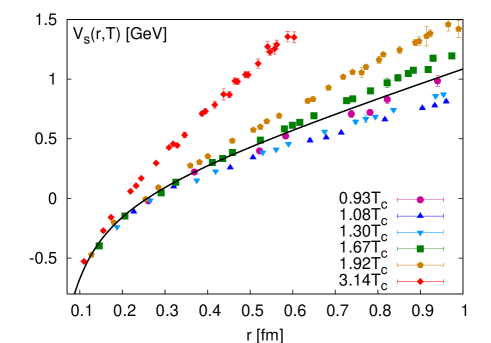
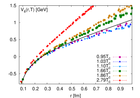
Let us first discuss the most prominent features of the spatial potential at finite temperatures and compare it to the usual zero temperature potential. Note that for the zero temperature lattices, of course, timelike and spatial Wilson loops are identical. In Figure 1 we show the spatial potential calculated for and at a few selected values of the temperature. We have subtracted the renormalization constant determined at zero temperature in Ref. eos_paper to make the comparison between different temperatures easier. Figure 1 shows that below the spatial Wilson loop shows very little change with temperature, while above the transition temperature a strong temperature dependence is seen. Only at very short distances the spatial potential remains, within errors, temperature independent also above . For temperatures close to the transition temperature the spatial potential falls below the zero temperature potential. The effect is more pronounced for than for which might indicate that this is a cut-off effect. As the temperature increases the slope of the spatial potential at large distances, i.e. the spatial string tension, clearly increases in agreement with observations made previously in pure gauge theories. This will be discussed in more detail in the next section.
We find no evidence of string breaking occurring in the high temperature spatial potentials. This, however, may not be too surprising as it is known from studies of the heavy quark potential at zero temperature that smeared Wilson loops at numerically accessible perimeters are not well suited for studying string breaking. Polyakov loop correlation functions have been found to perform much better in this respect deTar . Therefore one might want to also analyze spatial Polyakov loop correlation functions to get more sensitive to string breaking effects in spatial potentials.
IV Spatial string tension
In order to extract the spatial string tension from the large distance behavior of the spatial pseudo-potentials we have to rely on fits. However, the choice of an appropriate fit Ansatz is less obvious than at zero temperature. At zero and low temperatures the (pseudo-) potential is usually well described by
| (6) |
The term, in dimensions, may arise from two contributions, from Coulombic perturbative gluon exchange at small distances, approximately fm, and from string fluctuations relevant at distances fm. The later is often referred to as the Lüscher term. In fact, in the proportionality factor of the string fluctuation term, , is a universal constant,
| (7) |
that only depends on the space-time dimensionality Luescher . As dimensional reduction manifests itself as temperature increases one should expect that the contribution arising from string fluctuations should gradually turn from to . In fact, finite temperature corrections to the string fluctuation term have been calculated previously deForcrand and have been found to be of relevance for the analysis of the temperature dependence of the (conventional) heavy quark potential Kaczmarek . At the same time and for the same reason, the Coulombic term due to perturbative gluon exchange is expected to change from a behavior appropriate in 4 dimensions to a logarithmic dependence in an effectively 3 dimensional theory. It is this gradual change in the short and intermediate distance part of the pseudo-potential that is responsible for ambiguities in the fit Ansatz. We will discuss in the following our strategy to deal with this ambiguity.
From our data, we could not clearly disentangle a term from a behavior. In fact, addition of the term to the form of Eq. (6) only makes the fit very noisy. Similarly we could not restrict the fit intervals to such large distances where terms of whatever origin, Coulombic or string fluctuations, could be safely neglected. We therefore have fitted our data to Eq.(6) with 3 free parameters. We note that this is not too severe a restriction as we are not interested in a detailed description of the -dependence of the pseudo-potentials but rather want to get control over its large distance behavior.
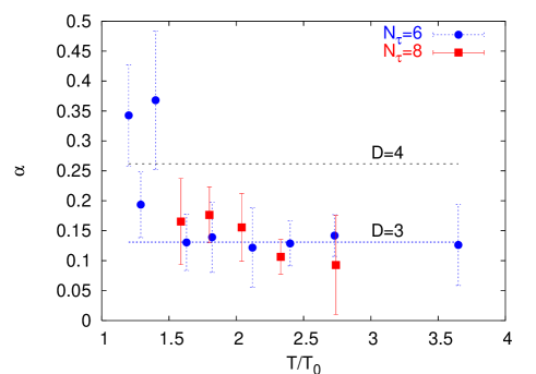
On our finer lattices ( and ) we observe that the coefficient of the term, i.e. , decreases with increasing temperature and approaches at high temperatures. This is shown in Figure 2. The fit results for are somewhat dependent on the fit range. We have adopted to choose a minimum separation between and times .
At sufficiently large distances the Coulombic term will not be seen, with only string fluctuations contributing. Fixing the value of to the coefficient of the Lüscher term, , may describe the potential at large distances. This Ansatz was fitted to the potential at distances greater than . For small temperatures, , with fixed to the values of coming from these 2 parameter fits are systematically larger than those coming from the 3 parameter fits. At high temperatures, however, the spatial string tension obtained from two parameter fits with and three parameter fits agree within statistical errors.
The values of the spatial string tension for different are summarized in Table 1. For and the string tension has been determined from 3 parameter fits. For the case we used mostly two parameter fits with different values of . The errors on the spatial string tension shown in the table are predominantly systematic due to the choice of the fit form and fit interval. The temperature dependence of the spatial string tension is shown in Figure 3.
For temperatures the spatial string tension is close to the zero temperature string tension and is linearly rising with temperature for This is expected if dimensional reduction holds at these temperature values. We will discuss this in more detail in the next section. It is possible that also the rapid drop in the coefficient of the Coulomb term for is related to the onset of the 3-dimensional physics reflected in the linear rise of the spatial string tension in this temperature region.
| 3.150 | 0.367(18) | 0.535(36) | 3.43 | 0.441(1) | 0.156(5) | 3.53 | 0.458(4) | 0.0905(7) |
|---|---|---|---|---|---|---|---|---|
| 3.210 | 0.396(9) | 0.577(33) | 3.46 | 0.482(3) | 0.123(3) | 3.57 | 0.501(3) | 0.0722(11) |
| 3.240 | 0.417(8) | 0.458(27) | 3.47 | 0.511(3) | 0.103(7) | 3.585 | 0.520(13) | 0.0695(29) |
| 3.277 | 0.449(5) | 0.406(21) | 3.49 | 0.537(5) | 0.102(5) | 3.76 | 0.756(8) | 0.0486(12) |
| 3.335 | 0.500(3) | 0.254 (10) | 3.51 | 0.571(10) | 0.101(7) | 3.82 | 0.858(12) | 0.0435(6) |
| 3.351 | 0.517(3) | 0.244 (12) | 3.54 | 0.615(6) | 0.100(5) | 3.92 | 0.974(9) | 0.0375(6) |
| 3.382 | 0.556(3) | 0.203(13) | 3.57 | 0.668(4) | 0.084(4) | 4.00 | 1.110(10) | 0.0357(6) |
| 3.410 | 0.626(5) | 0.195(8) | 3.63 | 0.775(7) | 0.087(2) | 4.08 | 1.304(28) | 0.0319(7) |
| 3.460 | 0.723(4) | 0.181(5) | 3.69 | 0.867(8) | 0.078(2) | |||
| 3.490 | 0.806(8) | 0.167(6) | 3.76 | 1.008(10) | 0.067(2) | |||
| 3.510 | 0.856(15) | 0.165(4) | 3.82 | 1.144(15) | 0.0610(6) | |||
| 3.540 | 0.922(9) | 0.152(6) | 3.92 | 1.298(11) | 0.0544(5) | |||
| 3.570 | 1.002(7) | 0.139(5) | 4.08 | 1.738(37) | 0.0465(7) | |||
| 3.630 | 1.163(10) | 0.135(5) | ||||||
| 3.690 | 1.300(12) | 0.126(6) | ||||||
| 3.760 | 1.513(15) | 0.111(5) | ||||||
| 3.820 | 1.688(24) | 0.104(3) | ||||||
| 3.920 | 1.947(17) | 0.094(2) | ||||||
V Comparison with the prediction of dimensionally reduced theory
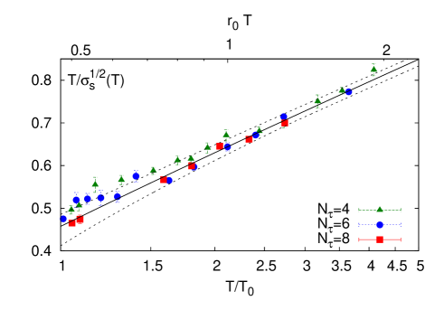
As has been discussed in Section II we expect that at high temperatures the spatial string tension should be given by . At temperatures several orders of magnitude larger than the transition temperature, when the static electric field can be integrated out, the effective theory is just a pure SU(3) gauge theory. The proportionality coefficient is just a constant and has been determined to be teper , corroborating an earlier value of bielefeld . In the interesting temperature range of a few times , however, will depend on the mass and coupling of the field and thus on the temperature. In the light of the approximate decoupling of the 3d scalar and gauge fields we expect that the dependence of the coefficient on these parameters should be weak and its value should be close to the pure gauge value given above. Indeed, the calculations of the string tension in 3-dimensional adjoint Higgs models show only a weak dependence on the parameters of the scalar sector and its value is close to the pure gauge value hart . Unfortunately, the statistical accuracy of the spatial string tension calculated in the 3d adjoint Higgs model is significantly lower than in the pure gauge case and no continuum extrapolation has been performed. For the relevant case of three quark flavors and temperatures of about the value of is about lower than the pure gauge value at fixed lattice spacing corresponding to . The analysis of Ref. hart also suggests that a possible temperature dependence of is less than . Therefore we use an averaged value in our analysis, where the indicated uncertainty also includes possible temperature dependence in it.
The gauge coupling of the effective 3d theory has been calculated to 2-loop accuracy mikko
| (8) | |||||
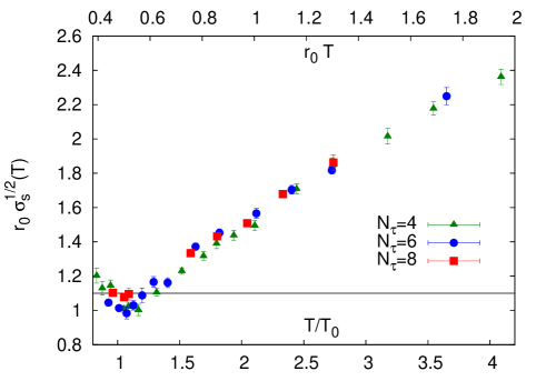
Here is the QCD coupling in scheme, and are the coefficients of the universal 2-loop beta function, and is the renormalization scale. The coefficients and can be found in Ref. mikko . In our case . The coupling depends on the renormalization scale at any fixed order of perturbation theory. Of course, the dependence on gets weaker and weaker as we go to higher orders of the perturbative expansion. In practice, however, we have to deal with the scale dependence of the effective coupling. Following Ref. mikko we fix the scale using the principle of minimum sensitivity, i.e. we require that the derivative of the 1-loop expression for vanishes at , and vary the scale in the interval . For 3-flavor QCD we find the value . To specify and thus completely we need to know the value of , or more precisely the ratio . Since the temperature has been set by the Sommer parameter this means that we need to specify . This can be done in principle by calculating the parameter at several lattice spacings and fitting it by the modified 2-loop Ansatz alton to determine . One then may use lattice perturbation theory to calculate . This has been done in SU(3) gauge theory capitani as well as in 2-flavor QCD with Wilson fermions goeckeler . Unfortunately, the perturbative calculations needed for this have not been performed for the p4fat3 action. On the other hand we can express the temperature in physical units using the Sommer parameters fm obtained from quarkonium splitting as input gray . Furthermore, using the same physical input the running coupling constant has been calculated on the lattice in 2+1 flavor QCD within the so-called scheme mason , giving . This corresponds to if we use the 3-loop relation york between the coupling in the -scheme and the -scheme. Using the 2-loop beta function we can determine the coupling entering Eq. (8) at the given scale thus specifying the gauge coupling of the effective 3d theory for different temperatures. Combining the value of from above and we finally get the corresponding prediction for the spatial string tension in the dimensionally reduced theory. In Figure 4 we show our results for compared with the prediction coming from the dimensionally reduced theory as discussed above. This is shown as a solid line with its uncertainty shown as a band (dashed lines). There are three sources of uncertainty in the dimensional reduction prediction. The first is the uncertainty in the value of . This is the dominant source of the error at high temperatures, . The second source of error is the scale dependence of , which is the most important one at low temperatures, . Finally there is an error in coming from the value of . This, however, is significantly smaller than the previous two in the entire temperature range.
Figure 4 seems to suggest that dimensional reduction works down to temperatures surprisingly close to the transition temperature. In order to see whether this picture is self-consistent one has to calculate other spatial correlation functions. In particular, one has to verify that the largest correlation length of operators built from quarks is sufficiently small to justify integrating out the Matsubara modes of quarks. In Ref. gavai this problem has been studied in 4-flavor QCD, using lattices with the standard staggered formulation. The analysis performed in that paper suggests that the pion correlator gives the largest correlation length up to temperatures as high as . Note, however, that this may be due to large discretization errors in the screening masses when the standard staggered action is used on lattices. Indeed, for this action it has been noticed in Ref. gavai03 that the pion screening masses on lattices may come close to a value of . Recent preliminary calculations with improved (p4fat3) staggered fermions mukherjee ; mscr_unpub give large values for this quantity, for and for , already on lattices with and . Thus the value of the pion screening mass is larger than the smallest glueball screening mass for which was estimated to be gavai and larger than the Debye screening mass estimated in mD2+1f . This indeed would suggest that in QCD dimensional reduction may work down to temperatures as low as also in the case of 2+1 flavor.
VI Conclusions
In this paper we have calculated the spatial string tension in 2+1 flavor QCD with a physical strange quark mass and light quark masses of corresponding to a pion mass of about MeV. The spatial string tension calculated at different lattice spacings agree reasonably well with each other. We have compared the results of our calculation with the prediction of dimensionally reduced effective theory and have found remarkably good agreement down to temperatures close to the transition temperature. This is similar to the observation made in SU(3) gauge theory mikko . There are three sources of uncertainty when comparing the data on the spatial string tension the scale dependence of the 3d gauge coupling, the uncertainty in the value of coefficient and the uncertainty in . The uncertainties from the last two sources could be reduced by calculating the lattice beta function for the p4fat3 action perturbatively and through a more precise calculation of the string tension of the 3d adjoint Higgs model.
Let us finally note that the spatial string tension has been recently studied also in 2 flavor QCD using Wilson fermions and significantly larger quark masses bornyakov ; maezawa . In Ref. bornyakov the spatial string tension has been calculated only up to and no temperature dependence has been found in this temperature interval. The results of Ref. maezawa , obtained on lattices with temporal extent qualitatively agree with ours, but the drop of the string tension close to is significantly larger. It remains to be seen to what extent these discrepancies are due to larger quark mass, cutoff effects or limited statistics, as calculations with Wilson fermions are numerically more demanding.
Acknowledgements
EL and JL wish to thank Y. Schröder for helpful discussions. This work has been supported in part by contracts DE-AC02-98CH1-0886 and DE-FG02-92ER40699 with the U.S. Department of Energy, by the Bundesministerium für Bildung und Forschung under grant 06BI401, the Gesellschaft für Schwerionenforschung by contract BILAER and the Deutsche Forschungsgemeinschaft under grant GRK 881. Calculations reported here were carried out using the QCDOC supercomputers of the RIKEN-BNL Research Center and the U.S. DOE, apeNEXT supercomputer at Bielefeld University, and the BlueGene/L (NYBlue) at the New York Center for Computational Sciences at Stony Brook University/Brookhaven National Laboratory which is supported by the U.S. Department of Energy under Contract No. DE-AC02-98CH10886 and by the State of New York.
References
- (1) C. Bernard et al., [MILC Coll.], Phys. Rev. D 71 (2005) 034504.
- (2) Y. Aoki et al., Nature 443 (2006) 675.
- (3) M. Cheng et al., Phys. Rev. D 74 (2006) 054507.
- (4) C. X. Zhai and B. M. Kastening, Phys. Rev. D 52 (1995) 7232.
- (5) P. Arnold and C. X. Zhai, Phys. Rev. D 51 (1995) 1906.
- (6) F. Karsch, A. Patkós and P. Petreczky, Phys. Lett. B 401 (1997) 69.
- (7) J.-P. Blaizot, E. Iancu and A. Rebhan, Phys. Rev. D 63 (2001) 065003.
- (8) J. O. Andersen et al., Phys. Rev. D 66 (2002) 085016.
- (9) A. Linde, Phys. Lett. B 96 (1980) 289.
- (10) C. DeTar, Phys. Rev. D 32 (1985) 276.
- (11) E. Manousakis and J. Polonyi, Phys. Rev. Lett. 58 (1987) 847.
- (12) G. S. Bali et al., Phys. Rev. Lett. 71 (1993) 3059.
- (13) F. Karsch, E. Laermann and M. Lütgemeier, Phys. Lett. B 346 (1995) 94.
- (14) G. Boyd et al., Nucl. Phys. B 469 (1996) 419.
- (15) M. Laine and Y. Schröder, JHEP 0503 (2005) 067; Y. Schröder and M. Laine, PoS LAT2005 (2006) 180.
- (16) R. Gavai and S. Gupta, Phys. Rev. Lett. 85 (2000) 2068.
- (17) T. Umeda, PoS LAT2006 (2006) 151 J. Liddle, PoS LAT2007 (2007) 204; F. Karsch, Nucl. Phys. A 783 (2007) 13.
- (18) T. Appelquist and R. Pisarski, Phys. Rev. D 23 (1981) 2305.
- (19) E. Braaten and A. Nieto, Phys. Rev. D 51 (1995) 6990.
- (20) K. Kajantie et al., Nucl. Phys. B 503 (1997) 357.
- (21) F. Karsch et al, Phys.Lett. B 442 (1998) 291.
- (22) P. Giovannangeli, Phys. Lett. B 585 (2004) 144
- (23) K. Kajantie et al., Phys. Rev. D 67 (2003) 105008.
- (24) B. Lucini and M. Teper, Phys. Rev. D 66 (2002) 097502.
- (25) A. Cucchieri, F. Karsch and P. Petreczky, Phys.Rev.D 64 (2001) 036001.
- (26) S. Datta and S. Gupta, Phys. Rev. D 67 (2003) 054503.
- (27) A. Hart and O. Philipsen, Nucl. Phys.B 572 (2000) 243. A. Hart. O. Philipsen and M. Laine, Nucl. Phys. B 586 (2000) 443.
- (28) M. Laine and M. Vepsäläinen, JHEP 0402 (2004) 004.
- (29) M. Cheng et al., Phys. Rev. D 77 (2008) 014511.
- (30) F. Karsch, E. Laermann and A. Peikert, Phys. Lett. B 478 (2000) 447.
- (31) R. Sommer, Nucl. Phys. B 411 (1994) 839.
- (32) A. Gray et al., Phys. Rev. D 72 (2005) 094507.
- (33) B. Bolder et al., Phys. Rev. D 63 (2001) 074504.
- (34) M. Creutz, Quarks, Gluons, and Lattices, Cambridge University press.
- (35) C. E. DeTar et al., Phys. Rev. D 59 (1999) 031501.
- (36) M. Lüscher, K. Symanzik and P. Weisz, Nucl. Phys. B 173 (1980) 365; M. Lüscher, Nucl. Phys. B 180 (1981) 317.
- (37) P. de Forcrand et al., Phys. Lett. B 160 (1985) 137.
- (38) O. Kaczmarek et al., Phys. Rev. D 62 (2000) 034021.
- (39) C. Allton, Nucl. Phys. B (Proc. Suppl.) 53 (1997) 867.
- (40) S. Capitani et al., [ALPHA Coll.], Nucl. Phys. B 544 (1998) 669.
- (41) M. Göckeler et al., Phys. Rev. D 73 (2006) 014513.
- (42) Q. Mason et al., Phys. Rev. Lett. 95 (2005) 052002.
- (43) Y. Schröder, Phys. Lett. B 447 (1999) 321.
- (44) R. V. Gavai and S. Gupta, Phys. Rev. D 67 (2003) 034501.
- (45) S. Mukherjee, PoS LAT2007 (2007) 210.
- (46) S. Datta et al (RBC-Bielefeld Coll.), in preparation
- (47) K. Petrov [RBC-Bielefeld Coll.], PoS LAT2007 (2007) 217; O. Kaczmarek, PoS CPOD07 (2007) 043.
- (48) V.G. Bornyakov and E.V. Lushchevskaya, arXiv:0706.3125
- (49) Y. Maezawa et al., [WHOT-QCD Coll.], Phys. Rev. D 75 (2007) 074501.