Gale duality and Koszul duality

Abstract.

Given a hyperplane arrangement in an affine space equipped with a linear functional, we define two finite-dimensional, noncommutative algebras, both of which are motivated by the geometry of hypertoric varieties. We show that these algebras are Koszul dual to each other, and that the roles of the two algebras are reversed by Gale duality. We also study the centers and representation categories of our algebras, which are in many ways analogous to integral blocks of category $\mathcal{O}$.

1. Introduction

In this paper we define and study a class of finite-dimensional graded algebras which are related to the combinatorics of hyperplane arrangements and to the geometry of hypertoric varieties. The categories of representations of these algebras are similar in structure to the integral blocks of category ${\cal O}$, originally introduced by Bernstein-Gelfand-Gelfand [BGG76]. Our categories share many important properties with such blocks, including a highest weight structure, a Koszul grading, and a relationship with the geometry of a symplectic variety. As with category ${\cal O}$, there is a nice interpretation of Koszul duality in our setting, and there are interesting families of functors between our categories. In this paper we take a combinatorial approach, analogous to that taken by Stroppel in her study of category ${\cal O}$ [Str03]. In a subsequent paper [BLPWa] we will take an approach to these categories more analogous to the classical perspective on category ${\cal O}$; we will realize them as categories of modules over an infinite dimensional algebra, and as a certain category of sheaves on a hypertoric variety, related by a localization theorem extending that of Beilinson-Bernstein [BB81].

1.1.

To define our algebras, we take as our input what we call a polarized arrangement ${\cal V}=(V,\eta,\xi)$, consisting of a linear subspace $V$ of a coordinate vector space ${\mathbb{R}}^{I}$, a vector $\eta\in{\mathbb{R}}^{I}/V$, and a covector $\xi\in V^{*}$. It is convenient to think of these data as describing an affine space $V_{\eta}\subseteq{\mathbb{R}}^{I}$ given by translating $V$ away from the origin by $\eta$, together with an affine linear functional on $V_{\eta}$ given by $\xi$ and a finite hyperplane arrangement ${\cal H}$ in $V_{\eta}$, whose hyperplanes are the restrictions of the coordinate hyperplanes in ${\mathbb{R}}^{I}$.

If ${\cal V}$ is rational, meaning that $V$, $\eta$, and $\xi$ are all defined over ${\mathbb{Q}}$, then we may associate to ${\cal V}$ a hyperkähler orbifold $\mathfrak{M}_{\cal H}$ called a hypertoric variety. The hypertoric variety depends only on the arrangement ${\cal H}$ (that is, on $V$ and $\eta$). It is defined as a hyperkähler quotient of the quaternionic vector space ${\mathbb{H}}^{n}$ by an $(n-\operatorname{dim}V)$-dimensional real torus determined by $V$, where the quotient parameter is specified by $\eta$. By fixing one complex structure on $\mathfrak{M}_{\cal H}$ we obtain an algebraic symplectic variety which carries a natural hamiltonian action of an algebraic torus with Lie algebra $V^{*}_{\mathbb{C}}$, and $\xi$ determines a one-dimensional subtorus. The definitions and results of this paper do not require any knowledge of hypertoric varieties (indeed, they will hold even if ${\cal V}$ is not rational, in which case there are no varieties in the picture). They will, however, be strongly motivated by hypertoric geometry, and we will take every opportunity to point out this motivation. The interested reader can learn more about hypertoric varieties in the survey [Pro08].

Given a polarized arrangement ${\cal V}$, we give combinatorial definitions of two quadratic algebras, which we denote by $A=A({\cal V})$ and $B=B({\cal V})$. If ${\cal V}$ is rational, both rings have geometric interpretations. The ${\mathbb{C}}^{*}$-action on $\mathfrak{M}_{\cal H}$ given by $\xi$ determines a lagrangian subvariety $\mathcal{X}\subset\mathfrak{M}_{\cal H}$, consisting of all points $x$ for which $\lim_{\lambda\to\infty}\lambda\cdot x$ exists. In this case, $B$ is isomorphic to the direct sum of the cohomology rings of all pairwise intersections of components of $\mathcal{X}$, equipped with a convolution product (Proposition 4.10). On the other hand, we will show in a forthcoming paper [BLPWa] that $A$ is the endomorphism algebra of a projective generator of a category of modules over a quantization of the structure sheaf of $\mathfrak{M}_{\cal H}$ which are supported on $\mathcal{X}$. This construction is motivated by geometric representation theory: the analogous category of modules on $T^{*}(G/B)$, the cotangent bundle of a flag variety, is equivalent to a regular block of category ${\cal O}$ for the Lie algebra $\mathfrak{g}$.

1.2.

There are two forms of duality lurking in this picture, one coming from combinatorics and the other from ring theory. We define the Gale dual of a polarized arrangement ${\cal V}=(V,\eta,\xi)$ as the triple

$${\cal V}^{\vee}=(V^{\perp},-\xi,-\eta),$$

where $V^{\perp}\subseteq({\mathbb{R}}^{I})^{*}$ is the space of linear forms on ${\mathbb{R}}^{I}$ that vanish on $V$. On the other hand, to any quadratic algebra $E$ we may associate its quadratic dual algebra $E^{!}$. We show that the algebras $A$ and $B$ are dual to each other in both of these senses:

Theorem (A).

There are ring isomorphisms $A({\cal V})^{!}\cong A({\cal V}^{\vee})$ and $A({\cal V}^{\vee})\cong B({\cal V})$.

We prove the following three facts about the rings $A$ and $B$, all of which are analogous to results about category ${\cal O}$ and the geometry of the Springer resolution [Spa76, Irv85, Bru08, Stra, SW].

Theorem (B).

1. The algebras $A$ and $B$ are quasi-hereditary and Koszul (and thus are Koszul dual).

2. If ${\cal V}$ is rational, then the center of $B$ is canonically isomorphic to the cohomology ring of $\mathfrak{M}_{\cal H}$.

3. There is a canonical bijection between indecomposible projective-injective $B$-modules and compact chambers of the hyperplane arrangement ${\cal H}$; if ${\cal V}$ is rational, these are in bijection with the set of all irreducible projective lagrangian subvarieties of $\mathfrak{M}_{{\cal H}}$.

Part (2) of Theorem (B) is analogous to a result of [Bru08, Stra], which says that the center of a regular block of parabolic category ${\cal O}$ for $\mathfrak{g}=\mathfrak{sl}_{n}$ is isomorphic to the cohomology of a Springer fiber. Note that the cohomology of the hypertoric variety $\mathfrak{M}_{\cal H}$ is independent of both parameters $\eta$ and $\xi$ [Kon00, HS02, Pro08]. This leads us to ask to what extent the algebras themselves depend on $\eta$ and $\xi$. It turns out that the algebras for polarized arrangements with the same underlying vector space $V$ may not be isomorphic or Morita equivalent, but they are derived Morita equivalent.

Theorem (C).

The bounded derived category of graded modules over $A({\cal V})$ or $B({\cal V})$ depends only on the subspace $V\subset{\mathbb{R}}^{I}$.

The functors that realize these equivalences are analogues of twisting and shuffling functors on category ${\cal O}$.

1.3.

The paper is structured as follows. In Section 2, we lay out the combinatorics and linear algebra of polarized arrangements, introducing definitions and constructions upon which we will rely throughout the paper. Section 3 is devoted to the algebra $A$, and contains a proof of the first isomorphism of Theorem (A). In Section 4 we turn to the algebra $B$; in it we complete the proof of Theorem (A), as well as part (2) of Theorem (B). Section 5 begins with a general overview of quasi-hereditary and Koszul algebras, culminating in the proofs of parts (1) and (3) of Theorem (B). In Section 6 we prove Theorem (C), and along the way we study Ringel duality, Serre functors, and mutations of exceptional collections of $A$-modules.

Let ${\cal H}^{\vee}$ be the hyperplane arrangement associated to ${\cal V}^{\vee}$. The relationship between the hypertoric varieties $\mathfrak{M}_{\cal H}$ and $\mathfrak{M}_{{\cal H}^{\vee}}$ implied by our results is a special case of a duality relating pairs of symplectic algebraic varieties. This duality, which we call symplectic duality, will be explored in a more general context in future papers [BLPWa, BLPWb]. Other examples of symplectic dual pairs include Springer resolutions for Langlands dual groups and certain pairs of moduli spaces of instantons on surfaces. These examples all appear as the Higgs branches of the moduli space of vacua for mirror dual 3-d $\mathcal{N}=4$ super-conformal field theories, or as the Higgs and Coulomb branches of a single such theory. For hypertoric varieties, this was shown by Strassler and Kapustin [KS99]. We anticipate that our results on symplectic duality will ultimately be related to the structure of these field theories.

Acknowledgments. The authors would like to thank Jon Brundan, Michael Falk, Davide Gaiotto, Sergei Gukov, Christopher Phan, Catharina Stroppel, and Edward Witten for invaluable conversations.

T.B. was supported in part by NSA grant H98230-08-1-0097. A.L. was supported in part by a Clay Liftoff Fellowship. N.P. was supported in part by NSF grant DMS-0738335. B.W. was supported by a Clay Liftoff Fellowship and an NSF Postdoctoral Research Fellowship. T.B. would like to thank the Institute for Advanced Studies of the Hebrew University, Jerusalem, and Reed College for their hospitality.

2. Linear programming

2.1. Polarized arrangements

Let $I$ be a finite set.

Definition 2.1.

A polarized arrangement indexed by $I$ is a triple ${\cal V}=(V,\eta,\xi)$ consisting of

• a vector subspace $V\subset{\mathbb{R}}^{I}$,

• a vector $\eta\in{\mathbb{R}}^{I}/V$, and

• a covector $\xi\in V^{*}=({\mathbb{R}}^{I})^{*}/V^{\perp}$,

such that

1. every lift of $\eta$ to ${\mathbb{R}}^{I}$ has at least $|I|-\operatorname{dim}V$ non-zero entries, and

2. every lift of $\xi$ to $({\mathbb{R}}^{I})^{*}$ has at least $\operatorname{dim}V$ non-zero entries.

(Note that for $V$ fixed, a generic $\eta$ will satisfy (a), and a generic $\xi$ will satisfy (b).) If $V$, $\eta$, and $\xi$ are all defined over ${\mathbb{Q}}$, then ${\cal V}$ is called rational.

Associated to a (not necessarily rational) polarized arrangement ${\cal V}=(V,\eta,\xi)$ is an arrangement ${\cal H}$ of $|I|$ hyperplanes in the affine space

$$V_{\eta}=\{x\in{\mathbb{R}}^{I}\mid\eta=x+V\},$$

whose $i^{\text{th}}$ hyperplane is given by

$$H_{i}=\{x\in V_{\eta}\mid x_{i}=0\}.$$

Note that $H_{i}$ could be empty if $V$ is contained in the coordinate hyperplane $\{x_{i}=0\}$. In that case we refer to $i$ as a loop of ${\cal V}$, since it represents a loop in the matroid associated to $V$.

For any subset $S\subset I$, we let

$$H_{S}=\bigcap_{i\in S}H_{i}$$

be the flat spanned by the set $S$. Condition (a) implies that ${\cal H}$ is simple, meaning that $\operatorname{codim}H_{S}=|S|$ whenever $H_{S}$ is nonempty. Observe that $\xi$ may be regarded as an affine-linear functional on $V_{\eta};$ it does not have well-defined values, but it may be used to compare any pair of points. Condition (b) implies that $\xi$ is generic with respect to the arrangement, in the sense that it is not constant on any positive-dimensional flat $H_{S}$.

2.2. Boundedness and feasibility

Given a sign vector $\alpha\in\{\pm 1\}^{I}$, let

$$\Delta_{\alpha}=V_{\eta}\cap\{x\in{\mathbb{R}}^{I}\mid\alpha(i)x_{i}\geq 0\;\text{for all $i$}\}$$

and

$$\Sigma_{\alpha}=V\cap\{x\in{\mathbb{R}}^{I}\mid\alpha(i)x_{i}\geq 0\;\text{for all $i$}\}.$$

If $\Delta_{\alpha}$ is nonempty, it is the closed chamber of the arrangement ${\cal H}$ where the defining equations of the hyperplanes are replaced by inequalities according to the signs in $\alpha$. The cone $\Sigma_{\alpha}$ is the corresponding chamber of the central arrangement given by translating the hyperplanes of ${\cal H}$ to the origin. It is always nonempty, as it contains $0$. If $\Delta_{\alpha}$ is nonempty, then $\Sigma_{\alpha}$ is the recession cone of $\Delta_{\alpha}$ — the set of direction vectors of rays contained in $\Delta_{\alpha}$ (see [Zie95, §1.5]). Note that $\Sigma_{\alpha}$ is independent of $\eta$, so even if $\Delta_{\alpha}=\varnothing$, it is possible to change $\eta$ (in terms of ${\cal H}$, this corresponds to translating the hyperplanes) to obtain a nonempty $\Delta_{\alpha}$, and then take its cone of unbounded directions.

We now define subsets ${\cal F},{\cal B},{\cal P}\subset\{\pm 1\}^{I}$ as follows. First we let

$${\cal F}=\{\alpha\in\{\pm 1\}^{I}\mid\Delta_{\alpha}\neq\varnothing\}.$$

Elements of ${\cal F}$ are called feasible. It is clear that ${\cal F}$ depends only on $V$ and $\eta$. Next, we let

$${\cal B}=\{\alpha\in\{\pm 1\}^{I}\mid\xi(\Sigma_{\alpha})\,\text{is bounded above}\}.$$

Elements of ${\cal B}$ are called bounded, and it is clear that ${\cal B}$ depends only on $V$ and $\xi$. Elements of the intersection

$${\cal P}:={\cal F}\cap{\cal B}=\{\alpha\in\{\pm 1\}^{I}\mid\xi(\Delta_{\alpha})\,\text{is nonempty and bounded above}\}$$

are called bounded feasible; here $\xi(\Delta_{\alpha})$ is regarded as a subset of the affine line. Our use of these terms comes from linear programming, where we consider $\alpha$ as representing the linear program “find the maximum of $\xi$ on the polyhedron $\Delta_{\alpha}$”.

Example 2.2.

Let $I=\{1,2,3,4\}$, and let ${\cal V}=(V,\eta,\xi)$ be the polarized arrangement where

$$V=\{(y,y,x,x+y)\mid(x,y)\in{\mathbb{R}}^{2}\},$$

$\eta$ is the image of $(-1,0,0,-2)$ in ${\mathbb{R}}^{4}/V$, and $\xi$ is the image of $(2,0,1,0)\in({\mathbb{R}}^{4})^{*}$ in $V^{*}=({\mathbb{R}}^{4})^{*}/V^{\bot}$. In terms of the $(x,y)$ coordinates on $V_{\eta}$, the inequalities defining the positive sides of the four hyperplanes are $y\geq 1$, $y\geq 0$, $x\geq 0$, and $x+y\geq 2$. The functional $\xi$, up to an additive constant, is $\xi(x,y)=x+2y$. See Figure 1, where we label all of the feasible regions with the appropriate sign vectors. The bounded feasible regions are shaded. Note that besides the five unbounded feasible regions pictured, there is one more unbounded sign vector, namely $+-++$, which is infeasible.

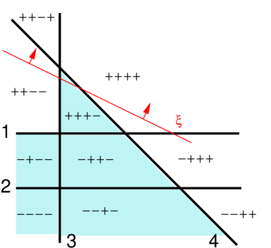
Figure 1. Example of bounded and feasible chambers

2.3. Gale duality

Here we introduce one of the two main dualities of this paper.

Definition 2.3.

The Gale dual ${\cal V}^{\vee}$ of a polarized arrangement ${\cal V}=(V,\eta,\xi)$ is given by the triple $(V^{\perp},-\xi,-\eta)$. We denote by ${\cal F}^{\vee}$, ${\cal B}^{\vee}$, and ${\cal P}^{\vee}$ the feasible, bounded, and bounded feasible sign vectors for ${\cal V}^{\vee}$, and we denote by $V^{\bot}_{-\xi}$ the affine space for the corresponding hyperplane arrangement ${\cal H}^{\vee}$.

This definition agrees with the notion of duality in linear programming: the linear programs for ${\cal V}$ and ${\cal V}^{\vee}$ and a fixed sign vector $\alpha$ are dual to each other. The following key result is a form of the strong duality theorem of linear programming.

Theorem 2.4.

${\cal F}^{\vee}={\cal B}$, $\,{\cal B}^{\vee}={\cal F}$, and therefore ${\cal P}^{\vee}={\cal P}$.

Proof.

It is enough to show that $\alpha=(+1,\dots,+1)$ is feasible for ${\cal V}$ if and only if it is bounded for ${\cal V}^{\vee}$. The Farkas lemma [Zie95, 1.8] says that exactly one of the following statements holds:

1. there exists a lift of $\eta$ to ${\mathbb{R}}^{I}$ which lies in ${\mathbb{R}}^{I}_{\geq 0}$,

2. there exists $c\in V^{\perp}\subset({\mathbb{R}}^{I})^{*}$ which is positive on ${\mathbb{R}}^{I}_{\geq 0}$ and negative on $\eta$.

Statement (1) is equivalent to $\alpha\in{\cal F}$, while a vector $c$ satisfying (2) lies in $\Sigma^{\vee}_{\alpha}$, so $c(\eta)<0$ means that $-\eta$ is not bounded above on $\Sigma^{\vee}_{\alpha}$. ∎

Example 2.5.

Continuing with polarized arrangement ${\cal V}$ of Example 2.2, we have

$$V^{\vee}=V^{\perp}=\{(X+Y,-X,Y,-Y)\mid(X,Y)\in{\mathbb{R}}^{2}\}.$$

So in $(X,Y)$ coordinates, the inequalities defining the positive sides of the four hyperplanes are, in order, $X+Y\geq 2$, $X\leq 0$, $Y\geq 1$, $Y\leq 0$ (the fact that these are the same as for ${\cal V}$ up to sign and reordering is a coincidence). The covector $\xi^{\vee}=-\eta$ gives the function $(X,Y)\mapsto X-Y$. Figure 2 shows the feasible and bounded feasible regions for ${\cal V}^{\vee}$.

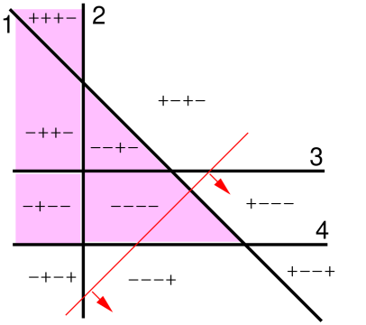
Figure 2. Bounded and feasible chambers for the Gale dual arrangement

2.4. Restriction and deletion

We define two operations which reduce the number of hyperplanes in a polarized arrangement as follows. First, consider a subset $S$ of $I$ such that $V+{\mathbb{R}}^{I\smallsetminus S}={\mathbb{R}}^{I}$. Since $\eta$ is assumed to be generic, this condition is equivalent to saying that $H_{S}\neq\varnothing$. Consider the natural isomorphism

$$i:{\mathbb{R}}^{I\smallsetminus S}/(V\cap{\mathbb{R}}^{I\smallsetminus S})\longrightarrow{\mathbb{R}}^{I}/V$$

induced by the inclusion of ${\mathbb{R}}^{I\smallsetminus S}$ into ${\mathbb{R}}^{I}$. We define a new polarized arrangement ${\cal V}^{S}=(V^{S},\xi^{S},\eta^{S})$, indexed by the set $I\smallsetminus S$, as follows:

$$V^{S} :=V\cap{\mathbb{R}}^{I\smallsetminus S}\subset{\mathbb{R}}^{I\smallsetminus S}$$

$$\xi^{S} :=\xi|_{V^{S}}$$

$$\eta^{S} :=i^{-1}(\eta).$$

The arrangement ${\cal V}^{S}$ is called the restriction of ${\cal V}$ to $S$, since the associated hyperplane arrangement is isomorphic to the hyperplane arrangement obtained by restricting to the subspace $H_{S}$.

Dually, suppose that $S\subset I$ is a subset such that ${\mathbb{R}}^{S}\cap V=\{0\}$, and let

$$\pi\colon{\mathbb{R}}^{I}\to{\mathbb{R}}^{I\smallsetminus S}$$

be the coordinate projection, which restricts to an isomorphism

$$\pi|_{V}:V\longrightarrow\pi(V).$$

We define another polarized arrangement ${\cal V}_{S}=(V_{S},\eta_{S},\xi_{S})$, also indexed by $I\smallsetminus S$, as follows:

$$V_{S} =\pi(V)\subset{\mathbb{R}}^{I\smallsetminus S}$$

$$\eta_{S} =\pi(\eta)$$

$$\xi_{S} =\xi\circ\pi|_{V}^{-1}.$$

The arrangement ${\cal V}_{S}$ is called the deletion of $S$ from ${\cal V}$, since the associated hyperplane arrangement is obtained by removing the hyperplanes $\{H_{i}\}_{i\in S}$ from the arrangement associated to ${\cal V}$. The following lemma is an easy consequence of the definitions.

Lemma 2.6.

$({\cal V}^{S})^{\vee}$ is equal to $({\cal V}^{\vee})_{S}$.

Example 2.7.

We continue with Examples 2.2 and 2.5. The deletion ${\cal V}_{\{3,4\}}$ is not defined, since ${\mathbb{R}}^{\{3,4\}}\cap V^{\bot}={\mathbb{R}}\cdot(0,0,-1,1)\neq 0$; this can be seen in Figure 1 because removing the hyperplanes $3$ and $4$ leaves hyperplanes whose normal vectors do not span. Dually, the restriction $({\cal V}^{\vee})^{\{3,4\}}$ is not defined, since $V^{\bot}+{\mathbb{R}}^{\{1,2\}}\neq{\mathbb{R}}^{4}$. This can be seen geometrically because $H_{\{3,4\}}=V^{\bot}_{-\xi}\cap{\mathbb{R}}^{\{1,2\}}$ is empty.

On the other hand, we can form the deletion ${\cal V}_{\{4\}}$; it gives an arrangement of three lines in a plane, with the first two parallel. On the dual side, $({\cal V}^{\vee})^{\{4\}}$ is an arrangement of two points on a line; the third hyperplane is a loop or empty hyperplane, since in the original arrangement ${\cal V}^{\vee}$ the hyperplanes $H_{3}$ and $H_{4}$ are parallel.

2.5. The adjacency relation

Define a relation $\leftrightarrow$ on $\{\pm 1\}^{I}$ by saying

$$\alpha\leftrightarrow\beta$$

if and only if $\alpha$ and $\beta$ differ in exactly one entry; if $\alpha,\beta\in{\cal F}$, this means that $\Delta_{\alpha}$ and $\Delta_{\beta}$ are obtained from each other by flipping across a single hyperplane. We will write $\alpha\overset{i}{\leftrightarrow}\beta$ to indicate that $\alpha$ and $\beta$ differ in the $i^{\text{th}}$ component of $\{\pm 1\}^{I}$. We will also denote this by $\beta=\alpha^{i}$. The following lemma says that an infeasible neighbor of a bounded feasible sign vector is feasible for the Gale dual system.

Lemma 2.8.

Suppose that $\alpha\notin{\cal F}$, $\beta\in{\cal P}$, and $\alpha\leftrightarrow\beta$. Then $\alpha\in{\cal F}^{\vee}$.

Proof.

Suppose that $\alpha\overset{i}{\leftrightarrow}\beta$. The fact that $\beta\in{\cal P}\subseteq{\cal F}$ tells us that $\Delta_{\beta}\neq\varnothing$, while $\Delta_{\alpha}=\varnothing$, thus

$$H_{i}\cap\Delta_{\beta}=\Delta_{\alpha}\cap\Delta_{\beta}=\varnothing.$$

From this we can conclude that

$$\Sigma_{\alpha}=\Sigma_{\beta}\cap\{x_{i}=0\}\subset\Sigma_{\beta}.$$

The fact that $\beta\in{\cal P}\subset{\cal B}$, tells us that $\xi(\Sigma_{\beta})$ is bounded above, thus so is $\xi(\Sigma_{\alpha})$. This in turn tells us that $\alpha\in{\cal B}$, which is equal to ${\cal F}^{\vee}$ by Theorem 2.4. ∎

2.6. Bases and the partial order

Let ${\mathbb{B}}$ be the set of subsets $b\subset I$ of order $\operatorname{dim}V$ such that $H_{b}\neq\varnothing$. Such a subset is called a basis for the matroid associated to ${\cal V}$, and in fact this property depends only on the subspace $V\subset{\mathbb{R}}^{I}$. A set $b$ is a basis if and only if the composition $V\hookrightarrow{\mathbb{R}}^{I}\twoheadrightarrow{\mathbb{R}}^{b}$ is an isomorphism, which is equivalent to saying that we have a direct sum decomposition ${\mathbb{R}}^{I}=V\oplus{\mathbb{R}}^{b^{c}}$, where we put $b^{c}=I\smallsetminus b$. We have a bijection

$$\mu:{\mathbb{B}}\to{\cal P}$$

taking $b$ to the unique sign vector $\alpha$ such that $\xi$ attains its maximum on $\Delta_{\alpha}$ at the point $H_{b}$.

The covector $\xi$ induces a partial order $\leq$ on ${\mathbb{B}}\cong{\cal P}$. It is the transitive closure of the relation $\preceq$, where $b_{1}\prec b_{2}$ if $|b_{1}\cap b_{2}|=|b_{1}|-1=\operatorname{dim}V-1$ and $\xi(H_{b_{1}})<\xi(H_{b_{2}})$. The first condition means that $H_{b_{1}}$ and $H_{b_{2}}$ lie on the same one-dimensional flat, so $\xi$ cannot take the same value on these two points.

Let ${\mathbb{B}}^{\vee}$ denote the set of bases of ${\cal V}^{\vee}$. We have a bijection $b\mapsto b^{c}$ from ${\mathbb{B}}$ to ${\mathbb{B}}^{\vee}$, since ${\mathbb{R}}^{I}=V\oplus{\mathbb{R}}^{b^{c}}$ if and only if ${\mathbb{R}}^{I}=V^{\bot}\oplus{\mathbb{R}}^{b}$. The next result says that this bijection is compatible with the equality ${\cal P}={\cal P}^{\vee}$ and the bijections $\mu\colon{\mathbb{B}}\to{\cal P}$ and $\mu^{\vee}\colon{\mathbb{B}}^{\vee}\to{\cal P}^{\vee}$.

Lemma 2.9.

For all $b\in{\mathbb{B}}$, $\mu(b)=\mu^{\vee}(b^{c})$.

Proof.

Let $b\in{\mathbb{B}}$. It will be enough to show that $\mu(b)=\alpha$ if and only if

1. the projection of $\alpha$ to $\{\pm 1\}^{b^{c}}$ is feasible for the restriction ${\cal V}^{b}$, and

2. the projection of $\alpha$ to $\{\pm 1\}^{b}$ is bounded for the deletion ${\cal V}_{b^{c}}$,

since Theorem 2.4 and Lemma 2.6 tell us that these conditions are interchanged by dualizing and swapping $b$ with $b^{c}$.

Note that ${\cal V}^{b}$ represents the restriction of the arrangement to $H_{b}$, which is a point. All of the remaining hyperplanes are therefore loops, whose positive and negative sides are either all of $H_{b}$ or empty. Condition (1) just says then that $H_{b}$ lies in the chamber $\Delta_{\alpha}$. Given that, in order for $H_{b}$ to be the $\xi$-maximum on $\Delta_{\alpha}$, it is enough that when all the hyperplanes not passing through $H_{b}$ are removed from the arrangement, the chamber containing $\alpha$ is bounded. But this is exactly the statement of condition (2), which completes the proof. ∎

The following lemma demonstrates that this bijection is compatible with our partial order.

Lemma 2.10.

Under the bijection $b\mapsto b^{c}$, the partial order on ${\mathbb{B}}^{\vee}$ is the opposite of the partial order on ${\mathbb{B}}$. That is, $b_{1}\leq b_{2}$ if and only if $b_{1}^{c}\geq b_{2}^{c}$.

Proof.

It will be enough to show that the generating relations $\prec$ are reversed. So take bases $b_{1}$, $b_{2}$ with $|b_{1}\cap b_{2}|=|b_{1}|-1$. Then there exist $i_{1}\in b_{1}$ and $i_{2}\in b_{2}$ such that $b_{2}=b_{1}\cup\{i_{2}\}\smallsetminus\{i_{1}\}$. We need to show that $\xi(H_{b_{1}})<\xi(H_{b_{2}})$ holds if and only if $\xi^{\vee}(H^{\vee}_{b^{c}_{1}})>\xi^{\vee}(H^{\vee}_{b^{c}_{2}})$. This reduces to the (easy) case where $|I|=2$ by replacing ${\cal V}$ with the polarized arrangement ${\cal V}^{b_{1}\cap b_{2}}_{(b_{1}\cup b_{2})^{c}}$ obtained by restricting to the one-dimensional flat spanned by $H_{b_{1}}$ and $H_{b_{2}}$ and then deleting all hyperplanes but $H_{i_{1}}$ and $H_{i_{2}}$. ∎

For $b\in{\mathbb{B}}$, define

$${\cal B}_{b}=\{\alpha\in\{\pm 1\}^{I}\mid\alpha(i)=\mu(b)(i)\,\,\text{for all $i\in b$}\}.$$

Note that ${\cal B}_{b}\subset{\cal B}$, and ${\cal B}_{b}$ depends only on $V$ and $\xi$. Geometrically, the feasible sign vectors in ${\cal B}_{b}$ are those such that $\Delta_{\alpha}$ lies in the “negative cone” defined by $\xi$ with vertex $H_{b}$. Dually, we define

$${\cal F}_{b}=\{\alpha\in\{\pm 1\}^{I}\mid\alpha(i)=\mu(b)(i)\,\,\text{for all $i\notin b$}\}={\cal B}^{\vee}_{b^{c}}$$

to be the set of sign vectors such that $H_{b}\in\Delta_{\alpha}$. In particular, ${\cal F}_{b}\subset{\cal F}$. We will need the following lemma in Section 5.

Lemma 2.11.

If $\mu(a)\in{\cal B}_{b}$, then $a\leq b$.

Proof.

Let $C$ be the negative cone of $\mu(b)$. Then $\mu(a)\in{\cal B}_{b}$ means that $H_{a}\in C$. Let $C^{\prime}$ be the smallest face of $C$ on which $H_{a}$ lives. We will prove the lemma by induction on $d=\operatorname{dim}C^{\prime}$. If $d=0$, then $a=b$ and we are done. Otherwise, there is a one-dimensional flat which is contained in $C^{\prime}$ and passes through $H_{a}$. Following it in the $\xi$-positive direction, it must leave $C^{\prime}$, since $C^{\prime}$ is $\xi$-bounded. The point where it exits will be $H_{c}$ for some basis $c$, and $a<c$ by construction. But $H_{c}$ lies on a face of $C$ of smaller dimension, so the inductive hypothesis gives $c\leq b$. ∎

Example 2.12.

We continue with Examples 2.2 and 2.5. Figure 3 gives Hasse diagrams for the partial orders on ${\mathbb{B}}$ and ${\mathbb{B}}^{\vee}$.

Figure 3. Partial order on ${\mathbb{B}}$ and ${\mathbb{B}}^{\vee}$

3. The algebra $A$

3.1. Definition of $A$

Fix a polarized arrangement ${\cal V}$, and consider the quiver $Q=Q({\cal V})$ with vertex set ${\cal F}$ and arrows $\{(\alpha,\beta)\mid\alpha\leftrightarrow\beta\}$. Note in particular that there is an arrow from $\alpha$ to $\beta$ if and only if there is an arrow from $\beta$ to $\alpha$. Let $P(Q)$ be the algebra of real linear combinations of paths in the quiver $Q$, generated by pairwise orthogonal idempotents $\{e_{\alpha}\mid\alpha\in{\cal F}\}$ along with edge paths $\{p(\alpha,\beta)\mid\alpha\leftrightarrow\beta\}$. We use the following notation: if $\alpha_{1}\leftrightarrow\alpha_{2}\leftrightarrow\dots\leftrightarrow\alpha_{k}$ is a path in the quiver, then we write

$$p(\alpha_{1},\alpha_{2},\dots,\alpha_{k}):=p({\alpha_{1},\alpha_{2}})\cdot p({\alpha_{2},\alpha_{3}})\cdot\ldots\cdot p({\alpha_{k-1},\alpha_{k}}).$$

Let $t_{i}\in V^{*}$ be the restriction to $V$ of the $i^{\text{th}}$ coordinate function on ${\mathbb{R}}^{I}$.

Definition 3.1.

We define $A=A({\cal V})$ to be the quotient of $P(Q)\otimes_{\mathbb{R}}\operatorname{Sym}V^{*}$ by the two-sided ideal generated by the following relations:

1. If $\alpha\in{\cal F}\smallsetminus{\cal P}$, then $e_{\alpha}=0$.
   

2. If four distinct elements $\alpha,\beta,\gamma,\delta\in{\cal F}$ satisfy $\alpha\leftrightarrow\beta\leftrightarrow\gamma\leftrightarrow\delta\leftrightarrow\alpha$, then

   $$p(\alpha,\beta,\gamma)=p(\alpha,\delta,\gamma).$$

3. If $\alpha,\beta\in{\cal F}$ and $\alpha\overset{i}{\leftrightarrow}\beta$, then

   $$p(\alpha,\beta,\alpha)=t_{i}e_{\alpha}.$$

We put a grading on this algebra by letting $\deg(e_{\alpha})=0$ for all $\alpha\in{\cal F}$, $\deg(p(\alpha,\beta))=1$ for all $\alpha\leftrightarrow\beta$, and $\deg(t_{i})=2$ for all $i\in I$.

Let $Q_{\cal P}$ be the subquiver of $Q$ consisting of the vertices that lie in ${\cal P}$ and all arrows between them. The following lemma tells us that $A$ is quadratic, meaning that $A$ is generated over $A_{0}$ by $A_{1}$, and that the only nontrivial relations are in degree 2.

Lemma 3.2.

The natural map $P(Q_{\cal P})\to A$ is surjective, and the kernel is generated in degree two.

Proof.

For any $\alpha\in{\cal F}$, define the set

$$I_{\alpha}:=\{i\in I\mid\Delta_{\alpha}\cap H_{i}\neq\varnothing\}=\{i\in I\mid\alpha^{i}\in{\cal F}\};$$

it indexes the codimension one faces of $\Delta_{\alpha}$. Then the $t_{i}$ for $i\in I_{\alpha}$ are normal vectors to those faces, and therefore span $V^{*}$. Thus for any $w\in V^{*}$, the corresponding element $w=\sum_{\alpha\in{\cal F}}we_{\alpha}$ of $A$ can be written in terms of paths $p(\alpha,\beta,\alpha)$, using the relation A3. So $A$ is a quotient of the full path algebra $P(Q)$, and then by the relation A1 it is also quotient of $P(Q_{\cal P})$. The relations for this presentation are generated by those of A2 (where the right side is understood to be $0$ if $\delta\notin{\cal P}$) along with linear relations among the various $p(\alpha,\beta,\alpha)$ coming from the relations among the covectors $t_{i}\in V^{*}$. ∎

Remark 3.3.

The upshot of Lemma 3.2 is that we could have given a presentation of $A$ that was more efficient than the one given in Definition 3.1, in the sense that it would have used fewer generators, all in degrees 0 and 1. The trade-off would have been that the relations A2 and A3 would each have needed to be split into cases, depending on whether or not $\beta$ is bounded. Furthermore, the map from $\operatorname{Sym}V^{*}$ to $A$ would have been less apparent in this picture.

Remark 3.4.

In a subsequent paper [BLPWa] we will show that, when ${\cal V}$ is rational, the category of right $A$-modules is equivalent to a category of modules over a quantization of the structure sheaf of the hypertoric variety $\mathfrak{M}_{\cal H}$. In the special case where $\mathfrak{M}_{\cal H}\cong T^{*}X$ is the cotangent bundle of a projective variety $X$, these are just $\mathcal{D}$-modules on $X$ (microlocalized to $T^{*}X$) whose characteristic varieties are contained in the conormal variety to a certain stratification of the base. More generally, the sheaves will be supported on the relative core of $\mathfrak{M}_{\cal H}$ (see Section 4.2), a lagrangian subvariety of $\mathfrak{M}_{\cal H}$ defined by $\xi$.

Remark 3.5.

The quiver $Q$ has appeared in the literature before; it is the Cayley graph of the Deligne groupoid of ${\cal H}$ [Par00]. Indeed, let $\tilde{A}({\cal V})$ be the quotient of $P(Q)\otimes_{\mathbb{R}}\operatorname{Sym}({\mathbb{R}}^{I})^{*}$ by the relations A1, A2, and $\tilde{\rm A}3$, where $\tilde{\rm A}3$ is obtained from A3 by replacing $t_{i}\in V^{*}$ with the $i^{\text{th}}$ coordinate function on ${\mathbb{R}}^{I}$. Let the Deligne semi-groupoid be the groupoid generated by paths in $Q$. Then $\tilde{A}({\cal V})$ is the quotient by $\{e_{\alpha}\mid\alpha\in{\cal F}\smallsetminus{\cal P}\}$ of the semi-groupoid algebra of the Deligne semi-groupoid, and

$$A\cong\tilde{A}\otimes_{\operatorname{Sym}({\mathbb{R}}^{I})^{*}}\operatorname{Sym}V^{*}\cong A\otimes_{\operatorname{Sym}V^{\perp}}{\mathbb{R}}.$$

3.2. Taut paths

We next establish a series of results that allow us to understand the elements of $A$ more explicitly. Though we do not need these results for the remainder of Section 3, they will be used in Sections 4 and 5.

Definition 3.6.

For a sequence $\alpha_{1},\dots,\alpha_{k}$ of elements of $\{\pm 1\}^{I}$ and an index $i\in I$, define

$$\theta_{i}(\alpha_{1},\dots,\alpha_{k})=\big{|}\{1<j<k\mid\alpha_{j}(i)\neq\alpha_{j+1}(i)=\alpha_{1}(i)\}\big{|}.$$

This counts the number of times the sequence crosses the $i^{\text{th}}$ hyperplane and returns to the original side.

Definition 3.7.

We say that a path $\alpha_{1}\leftrightarrow\alpha_{2}\leftrightarrow\dots\leftrightarrow\alpha_{k}$ in $Q$ is taut if it has minimal length among all paths from $\alpha_{1}$ to $\alpha_{k}$. This is equivalent to saying that the sign vectors $\alpha_{1}$ and $\alpha_{k}$ differ in exactly $k-1$ entries.

Proposition 3.8.

Let $\alpha_{1}\leftrightarrow\alpha_{2}\leftrightarrow\dots\leftrightarrow\alpha_{k}$ be a path in $Q$. Then there is a taut path

$$\alpha_{1}=\beta_{1}\leftrightarrow\beta_{2}\leftrightarrow\dots\leftrightarrow\beta_{d}=\alpha_{k}$$

such that

$$p(\alpha_{1},\dots,\alpha_{k})=p(\beta_{1},\dots,\beta_{d})\cdot\prod_{i\in I}t_{i}^{\theta_{i}}$$

in the algebra $A$, where $\theta_{i}=\theta_{i}(\alpha_{1},\alpha_{2},\dots,\alpha_{k})$.

Proof.

We can represent paths in the quiver geometrically by topological paths in the affine space $V_{\eta}$ in which ${\cal H}$ lives. Let $\phi\colon[0,1]\to V_{\eta}$ be a piecewise linear path with the property that for any $t\in[0,1]$, the point $\phi(t)$ lies in at most one hyperplane $H_{i}$, and the endpoints $\phi(0)$ and $\phi(1)$ lie in no hyperplanes. Such a path determines an element $p(\phi)=p(\gamma_{1},\dots,\gamma_{r})$ in the algebra $A$, where $\Delta_{\gamma_{1}},\dots,\Delta_{\gamma_{r}}$ are the successive chambers visited by $\phi$. We define $\theta(\phi)=\theta(\gamma_{1},\dots,\gamma_{r})$.

To represent our given element $p(\alpha_{1},\dots,\alpha_{k})$ as $p(\phi)$ for a path $\phi$, we choose points $x_{1},\dots,x_{k}$ with $x_{j}\in\Delta_{\alpha_{j}}$ and let $\phi$ be the concatenation of the line segments $\overline{x_{j}x_{j+1}}$. By choosing the points $x_{j}$ generically we can assume that for every $1<j<k$ the line segment $\overline{x_{1}x_{j}}$ only passes through one hyperplane at a time, the plane containing $x_{1}$, $x_{j}$, and $x_{j+1}$ contains no point which lies in more than two hyperplanes, and any line through $x_{j+1}$ contained in this plane contains at most one point which is in two hyperplanes.

Given such points $x_{i}$, we construct a piecewise linear homotopy $\phi_{t}$ from $\phi=\phi_{0}$ to a straight-line path $\phi_{1}$ from $x_{1}$ to $x_{k}$, by contracting the points $x_{2},\dots,x_{k-1}$ one at a time along a straight line segment to $x_{1}$. The sequence of chambers visited by the path changes only a finite number of times, and at each step it can change in two possible ways. First, when the line segment $\overline{x_{j}x_{j+1}}$ passes through the intersection of two hyperplanes, a sequence $\alpha\leftrightarrow\beta\leftrightarrow\gamma$ with $\alpha\neq\gamma$ is replaced by $\alpha\leftrightarrow\delta\leftrightarrow\gamma$ with $\delta\neq\beta$. The quiver relation A2  implies that the corresponding element in the algebra $A$ does not change.

Second, when the point $x_{j}$ passes through a hyperplane $H_{i}$, either the sequence of chambers visited by the path is left unchanged, or a loop $\alpha\leftrightarrow\beta\leftrightarrow\alpha$ is replaced by $\alpha$. In the latter case, the element of the algebra is multiplied by $t_{i}$, by relation A3  in the definition of the algebra $A$. This is also the only change which affects the numbers $\theta_{j}(\phi_{t})$; it decreases $\theta_{i}$ by one and leaves the other $\theta_{j}$ alone.

Thus $p(\phi)=p(\phi_{1})\cdot\prod_{i\in I}t_{i}^{\theta_{i}}$, and $\phi_{1}$ represents a taut path, since a line segment cannot cross any hyperplane more than once. ∎

Corollary 3.9.

Let

$$\alpha=\alpha_{1}\leftrightarrow\alpha_{2}\leftrightarrow\dots\leftrightarrow\alpha_{d}=\beta$$

and

$$\alpha=\beta_{1}\leftrightarrow\beta_{2}\leftrightarrow\dots\leftrightarrow\beta_{d}=\beta$$

be two taut paths between fixed elements $\alpha,\beta\in{\cal P}$. Then

$$p(\alpha_{1},\dots,\alpha_{k})=p(\beta_{1},\dots,\beta_{d}).$$

Proof.

The proof of Proposition 3.8 shows that we can write $p(\alpha_{1},\dots,\alpha_{k})=p(\phi_{1})$ and $p(\beta_{1},\dots,\beta_{d})=p(\phi_{2})$, where $\phi_{1}$ and $\phi_{2}$ are both straight-line paths from a point of $\Delta_{\alpha_{1}}$ to a point of $\Delta_{\alpha_{k}}$. These endpoints can be chosen arbitrarily from a dense open subset of $\Delta_{\alpha_{1}}\times\Delta_{\alpha_{k}}$, so we can take $\phi_{1}=\phi_{2}$. ∎

Corollary 3.10.

Consider an element

$$a=p\cdot\prod_{i\in I}t_{i}^{d_{i}}\in e_{\alpha}Ae_{\beta},$$

where $p$ is represented by a taut path from $\alpha$ to $\beta$ in $Q$. Suppose that $\gamma\in{\cal F}$ satisfies $\gamma(i)=\alpha(i)$ whenever $\alpha(i)=\beta(i)$ and $d_{i}=0$. Then $a$ can be written as an ${\mathbb{R}}$-linear combination of elements represented by paths in $Q$ all of which pass through $\gamma$.

In particular, if $\gamma\in{\cal F}\smallsetminus{\cal P}$, then $a=0$.

Proof.

Applying Proposition 3.8 and Corollary 3.9 we see that the composition of taut paths from $\alpha$ to $\gamma$ and from $\gamma$ to $\beta$ is equal in $A$ to $p\cdot\prod_{i\in I}t_{i}^{d^{\prime}_{i}}$, where $d^{\prime}_{i}$ is $1$ if $\alpha(i)=\beta(i)\neq\gamma(i)$ and is $0$ otherwise. The result follows since $d_{i}\geq d^{\prime}_{i}$ for all $i$ and for any $i$ with $d_{i}>d^{\prime}_{i}$ we can express $e_{\beta}t_{i}$ as a combination of paths $p(\beta,\beta^{\prime},\beta)$, as in Lemma 3.2. ∎

3.3. Quadratic duality

We conclude this section by establishing the first part of Theorem (A), namely that the algebras $A({\cal V})$ and $A({\cal V}^{\vee})$ are quadratic duals of each other. First we review the definition of quadratic duality. See [PP05] for more about quadratic algebras.

Let $R={\mathbb{R}}\{e_{\alpha}\mid\alpha\in{\cal I}\}$ be a ring spanned by finitely many pairwise orthogonal idempotents, and let $M$ be an $R$-bimodule. Let $T_{R}(M)$ be the tensor algebra of $M$ over $R$, and let $W$ be a sub-bimodule of $M\otimes_{R}M=T_{R}(M)_{2}$. For shorthand, we will write $M_{\alpha\beta}=e_{\alpha}Me_{\beta}$ and $W_{\alpha\beta}=e_{\alpha}We_{\beta}$. To this data is associated a quadratic algebra

$$E=T_{R}(M)\,\Big{/}\,T_{R}(M)\cdot W\cdot T_{R}(M).$$

The quadratic dual $E^{!}$ of $E$ is defined as the quotient

$$E^{!}=T_{R}(M^{*})\,\Big{/}\,T_{R}(M^{*})\cdot W^{\perp}\cdot T_{R}(M^{*}),$$

where $M^{*}$ is the vector space dual of $M$, and

$$W^{\perp}\subset M^{*}\otimes_{R}M^{*}\cong\big{(}M\otimes_{R}M\big{)}^{*}$$

is the space of elements that vanish on $W$. Note that dualizing $M$ interchanges the left and right $R$-actions, so that $(M_{\alpha\beta})^{*}=(M^{*})_{\beta\alpha}$. It is clear from this definition that there is a natural isomorphism $E^{!!}\cong E$.

As we saw in Lemma 3.2, the algebra $A({\cal V})$ is quadratic, where we take ${\cal I}={\cal P}$ and

$$M={\mathbb{R}}\{\,p(\alpha,\beta)\mid\alpha,\beta\in{\cal P}\,\,\text{such that}\,\,\alpha\leftrightarrow\beta\}.$$

The relations of type A2 from Definition 3.1 lie in $W_{\alpha\gamma}$, while relations of type A3 lie in $W_{\alpha\alpha}$. Since ${\cal P}^{\vee}={\cal P}$, the algebra $A({\cal V}^{\vee})$ for the Gale dual polarized arrangement has the same base ring $R$. The degree one generating sets are also canonically isomorphic, since the adjacency relations on ${\cal P}$ and ${\cal P}^{\vee}$ are the same. However, in order to keep track of which algebra is which, we will denote the generators of $A({\cal V}^{\vee})$ by $p^{\vee}(\alpha,\beta)$ and their span by $M^{\vee}$.

We want to show that $A({\cal V})$ and $A({\cal V}^{\vee})$ are quadratic dual rings, so we must define a perfect pairing

$$M\otimes M^{\vee}\to{\mathbb{R}}$$

to identify $M^{\vee}$ with $M^{*}$. An obvious way to do this would be to make $\{p^{\vee}(\alpha,\beta)\}$ the dual basis to $\{p(\alpha,\beta)\}$, but this does not quite give us what we need. Instead, we need to twist this pairing by a sign. Choose a subset $X$ of edges in the underlying undirected graph of $Q$ with the property that for any square $\alpha\leftrightarrow\beta\leftrightarrow\gamma\leftrightarrow\delta\leftrightarrow\alpha$ of distinct elements, an odd number of the edges of the square are in $X$. The existence of such an $X$ follows from the fact that our graph is a subgraph of the edge graph of an $n$-cube. Define a pairing $\langle\,,\rangle$ by putting

$$\langle\,p(\alpha,\beta),\,p^{\vee}(\beta,\alpha)\,\rangle=\begin{cases}-1&\text{if}\,\{\alpha,\beta\}\in X\\ 1&\text{if}\,\{\alpha,\beta\}\notin X\end{cases}$$

and

$$\langle\,p(\alpha,\beta),\,p(\delta,\gamma)\,\rangle=0$$

unless $\alpha=\gamma$ and $\beta=\delta$.

Theorem 3.11.

The above pairing induces an isomorphism $A({\cal V}^{\vee})\cong A({\cal V})^{!}$.

Proof.

Let $W\subset(M\otimes_{R}M)_{2}$ and $W^{\vee}\subset(M^{\vee}\otimes_{R}M^{\vee})_{2}$ be the spaces of relations of $A({\cal V})$ and $A({\cal V}^{\vee})$, respectively. We analyze each piece $W_{\alpha\gamma}$ and $W^{\vee}_{\gamma\alpha}$ for every pair $\alpha,\gamma\in{\cal P}$ which admit paths of length two connecting them. First consider the case $\alpha\neq\gamma$; they must differ in exactly two entries, so there are exactly two elements $\beta_{1},\beta_{2}$ in $\{\pm 1\}^{I}$ which are adjacent to both $\alpha$ and $\gamma$. Since we are assuming that there is a path from $\alpha$ to $\gamma$ in ${\cal P}$, at least one of the $\beta_{j}$ must be in ${\cal P}$.

If both $\beta_{1}$ and $\beta_{2}$ are in ${\cal P}$, then $e_{\alpha}M\otimes_{R}Me_{\gamma}$ is a two-dimensional vector space with basis $\{p(\alpha,\beta_{1})\otimes p(\beta_{1},\gamma),p(\alpha,\beta_{2})\otimes p(\beta_{2},\gamma)\}$, while $e_{\gamma}M\otimes_{R}Me_{\alpha}$ has a basis $\{p^{\vee}(\gamma,\beta_{1})\otimes p^{\vee}(\beta_{1},\alpha),p^{\vee}(\gamma,\beta_{2})\otimes p^{\vee}(\beta_{2},\alpha)\}$. Then the relation A2 gives

$$W_{\alpha\gamma}={\mathbb{R}}\{p(\alpha,\beta_{1})\otimes p(\beta_{1},\gamma)-p(\alpha,\beta_{2})\otimes p(\beta_{2},\gamma)\}\;\text{and}$$

$$W^{\vee}_{\gamma\alpha}={\mathbb{R}}\{p^{\vee}(\gamma,\beta_{1})\otimes p^{\vee}(\beta_{1},\alpha)-p^{\vee}(\gamma,\beta_{2})\otimes p^{\vee}(\beta_{2},\alpha)\},$$

and so $W^{\vee}_{\gamma\alpha}=(W_{\alpha\gamma})^{\perp}$ (this is where we use the signs in our pairing).

If $\beta_{1}\in{\cal P}$ and $\beta_{2}\notin{\cal P}$, then either $\beta_{2}\in{\cal F}\smallsetminus{\cal P}$ and $\beta_{2}\notin{\cal F}^{\vee}$ or $\beta_{2}\in{\cal F}^{\vee}\smallsetminus{\cal P}^{\vee}$ and $b_{2}\notin{\cal F}$. In the first case we get $W_{\alpha\gamma}=e_{\alpha}M\otimes_{R}Me_{\gamma}$ since $p(\alpha,\beta_{1},\gamma)=p(\alpha,\beta_{2},\gamma)=0$ in $A({\cal V})$ by relations A1 and A2. On the other hand $\beta_{2}\notin{\cal F}^{\vee}$ means that the relation A2 doesn’t appear on the dual side, so $W^{\vee}_{\gamma\alpha}=0=(W_{\alpha\gamma})^{\perp}$. The argument in the second case is the same, reversing the role of ${\cal V}$ and ${\cal V}^{\vee}$.

We have dealt with the case $\alpha\neq\gamma$, so suppose now that $\alpha=\gamma$. The vector space $e_{\alpha}M\otimes_{R}Me_{\alpha}$ has a basis consisting of the elements $p(\alpha,\alpha^{i})\otimes p(\alpha^{i},\alpha)$ where $i$ lies in the set

$$J_{\alpha}:=\{i\in I\mid\alpha^{i}\in{\cal P}\}.$$

(Recall that $\alpha^{i}$ is the element of $\{\pm 1\}^{I}$ which differs from $\alpha$ in precisely the $i^{\text{th}}$ entry.) Note that $J_{\alpha}$ is a subset of the set $I_{\alpha}$ defined in the proof of Lemma 3.2. Let $I^{\vee}_{\alpha}$ and $J^{\vee}_{\alpha}$ be the corresponding sets for ${\cal V}^{\vee}$, and note that $J^{\vee}_{\alpha}=J_{\alpha}$.

Using this basis we can identify $W_{\alpha\alpha}$ with a subspace of ${\mathbb{R}}^{J_{\alpha}}$, which we compute as follows. Given a covector $w\in({\mathbb{R}}^{I})^{*}\cong{\mathbb{R}}^{I}$, its image in $V^{*}$ is $\sum_{i\in I}w_{i}t_{i}$, so the relations among the $t_{i}$ in $\operatorname{Sym}(V^{*})$ are given by $V^{\bot}\subset({\mathbb{R}}^{I})^{*}\cong{\mathbb{R}}^{I}$. If $\sum_{i\in I}w_{i}t_{i}=0$ and $w_{i}=0$ for $i\notin I_{\alpha}$, then multiplying by $e_{\alpha}$ and using relation A1 and A3 gives

$$\sum_{i\in J_{\alpha}}w_{i}p(\alpha,\alpha^{i},\alpha)=\sum_{i\in I_{\alpha}}w_{i}p(\alpha,\alpha^{i},\alpha)=0.$$

Thus $W_{\alpha\alpha}$ is the projection of $V^{\perp}\cap{\mathbb{R}}^{I_{\alpha}}$ onto ${\mathbb{R}}^{J_{\alpha}}$. Alternatively, we can first project $V^{\perp}$ onto ${\mathbb{R}}^{I_{\alpha}^{c}\cup J_{\alpha}}$ and then intersect with ${\mathbb{R}}^{J_{\alpha}}$.

On the dual side, the space $W^{\vee}_{\alpha\alpha}$ of relations among loops at $\alpha$ is identified with a vector subspace of ${\mathbb{R}}^{J^{\vee}_{\alpha}}={\mathbb{R}}^{J_{\alpha}}$, namely the projection of $V\cap{\mathbb{R}}^{I^{\vee}_{\alpha}}$ onto ${\mathbb{R}}^{J^{\vee}_{\alpha}}$. This is the orthogonal complement of $W_{\alpha\alpha}$, since Lemma 2.8 implies that $I_{\alpha}\smallsetminus J_{\alpha}=I\smallsetminus I^{\vee}_{\alpha}$. Note that the signs we added to the pairing do not affect this, since we always have

$$\langle p(\alpha,\beta),p^{\vee}(\beta,\alpha)\rangle\cdot\langle p(\beta,\alpha),p^{\vee}(\alpha,\beta)\rangle=1.\qed$$

4. The algebra $B$

4.1. Combinatorial definition

In this section we define our second algebra $B({\cal V})$ associated to the polarized arrangement ${\cal V}=(V,\eta,\xi)$. Consider the polynomial ring ${\mathbb{R}}[u_{i}]_{i\in I}=\operatorname{Sym}{\mathbb{R}}^{I}$. We give it a grading by putting $\deg u_{i}=2$ for all $i$. For any subset $S\subset I$, let $u_{S}=\prod_{i\in S}u_{i}$.

Definition 4.1.

Given a subset $\Delta\subset V_{\eta}$, define graded rings

$$\tilde{R}_{\Delta}:=\operatorname{Sym}{\mathbb{R}}^{I}\big{/}\left\langle u_{S}\mid S\subset I\,\,\text{such that}\,\,H_{S}\cap\Delta=\varnothing\right\rangle$$

and

$$R_{\Delta}:=\tilde{R}_{\Delta}\otimes_{\operatorname{Sym}V}{\mathbb{R}},$$

where the map from $\operatorname{Sym}V$ to $\operatorname{Sym}{\mathbb{R}}^{I}$ is induced by the inclusion $V\hookrightarrow{\mathbb{R}}^{I}$, and the map $\operatorname{Sym}(V)\to{\mathbb{R}}$ is the graded map which kills $V$. We use the conventions that $u_{\varnothing}=1$ and $H_{\varnothing}=V_{\eta}$, which means that $R_{\Delta}=0$ if and only if $\Delta=\varnothing$. Notice that if $\Delta_{1}\subset\Delta_{2}$, then we have natural quotient maps $\tilde{R}_{\Delta_{2}}\to\tilde{R}_{\Delta_{1}}$ and $R_{\Delta_{2}}\to R_{\Delta_{1}}$.

There are only certain subsets that will interest us, and for each of these subsets we introduce simplified notation for the corresponding ring. We put

(1) $$\tilde{R}_{\cal H}=\tilde{R}_{V_{\eta}},$$

and for any $\alpha,\beta,\gamma,\delta\in{\cal F}$,

(2) $$\tilde{R}_{\alpha}=\tilde{R}_{\Delta_{\alpha}},\,\,\,\tilde{R}_{\alpha\beta}=\tilde{R}_{\Delta_{\alpha}\cap\Delta_{\beta}},\,\,\,\tilde{R}_{\alpha\beta\gamma}=\tilde{R}_{\Delta_{\alpha}\cap\Delta_{\beta}\cap\Delta_{\gamma}},\,\,\,\text{and}\,\,\,\tilde{R}_{\alpha\beta\gamma\delta}=\tilde{R}_{\Delta_{\alpha}\cap\Delta_{\beta}\cap\Delta_{\gamma}\cap\Delta_{\delta}}.$$

Finally, we let $R_{\cal H}$, $R_{\alpha}$. $R_{\alpha\beta}$, $R_{\alpha\beta\gamma}$, and $R_{\alpha\beta\gamma\delta}$ denote the tensor products of these rings with ${\mathbb{R}}$ over $\operatorname{Sym}(V)$.

Lemma 4.2.

The ring $\tilde{R}_{\cal H}$ is a free $\operatorname{Sym}(V)$-module of total rank $|{\mathbb{B}}|$, the number of bases of the matroid of $V$. For any intersection $\Delta$ of chambers of ${\cal H}$, the ring $\tilde{R}_{\Delta}$ is a free $\operatorname{Sym}(V)$-module of total rank $|{\mathbb{B}}_{\Delta}|$, where ${\mathbb{B}}_{\Delta}=\left|\{b\in{\mathbb{B}}\mid H_{b}\subset\Delta\}\right|$.

Proof.

Both of these rings are the face rings of shellable simplicial complexes, namely the matroid complex of ${\cal V}$ and the dual of the face lattice of $\Delta$, respectively. This implies that they are free over the symmetric algebra of some subspace of ${\mathbb{R}}^{I}$, with bases parametrized by the top-dimensional simplices, which are in bijection with ${\mathbb{B}}$ and ${\mathbb{B}}_{\Delta}$, respectively. The fact that the rings are free over $\operatorname{Sym}(V)$ specifically follows from the fact that $V$ projects isomorphically onto ${\mathbb{R}}^{b}$ for any basis $b$. ∎

As we will see in the next section, when the arrangement ${\cal V}$ is rational, the rings of Equations (1) and (2) can be interpreted as equivariant cohomology rings of algebraic varieties with torus actions, while their tensor products with ${\mathbb{R}}$ are the corresponding ordinary cohomology rings. (In particular, we will give a topological interpretation of Lemma 4.2 in Remark 4.9.) However, our main theorems will all be proved in a purely algebraic setting.

For $\alpha,\beta\in{\cal P}$, let

$$d_{\alpha\beta}=\big{|}\{i\in I\mid\alpha(i)\neq\beta(i)\}\big{|}.$$

If the intersection $\Delta_{\alpha}\cap\Delta_{\beta}$ is nonempty, then $d_{\alpha\beta}$ is equal to its codimension inside of $V_{\eta}$. For $\alpha,\beta,\gamma\in{\cal P}$, let

$$S(\alpha\beta\gamma)=\{i\in I\mid\alpha(i)=\gamma(i)\neq\beta(i)\}.$$

If $\alpha,\beta$, and $\gamma$ are all feasible, then $S(\alpha\beta\gamma)$ is the set of hyperplanes that are crossed twice by the composition of a pair of taut paths from $\alpha$ to $\beta$ and $\beta$ to $\gamma$.

Definition 4.3.

Given a polarized arrangement ${\cal V}$, let

$$B=B({\cal V}):=\bigoplus_{(\alpha,\beta)\in{\cal P}\times{\cal P}}R_{\alpha\beta}[-d_{\alpha\beta}].$$

We define a product operation

$$\star\colon B\otimes B\to B$$

via the composition

$$\lx@xy@svg{\hbox{\raise 0.0pt\hbox{\kern 22.07845pt\hbox{\ignorespaces\ignorespaces\ignorespaces\hbox{\vtop{\kern 0.0pt\offinterlineskip\halign{\entry@#!@&&\entry@@#!@\cr&&&&\crcr}}}\ignorespaces{\hbox{\kern-22.07845pt\raise 0.0pt\hbox{\hbox{\kern 0.0pt\raise 0.0pt\hbox{\hbox{\kern 3.0pt\raise 0.0pt\hbox{$\textstyle{R_{\alpha\beta}\otimes R_{\beta\gamma}\ignorespaces\ignorespaces\ignorespaces\ignorespaces}$}}}}}}}\ignorespaces\ignorespaces\ignorespaces\ignorespaces{}{\hbox{\lx@xy@droprule}}\ignorespaces{\hbox{\kern 46.07845pt\raise 0.0pt\hbox{\hbox{\kern 0.0pt\raise 0.0pt\hbox{\lx@xy@tip{1}\lx@xy@tip{-1}}}}}}{\hbox{\lx@xy@droprule}}{\hbox{\lx@xy@droprule}}{\hbox{\kern 46.07845pt\raise 0.0pt\hbox{\hbox{\kern 0.0pt\raise 0.0pt\hbox{\hbox{\kern 3.0pt\raise 0.0pt\hbox{$\textstyle{R_{\alpha\beta\gamma}\otimes R_{\alpha\beta\gamma}\ignorespaces\ignorespaces\ignorespaces\ignorespaces}$}}}}}}}\ignorespaces\ignorespaces\ignorespaces\ignorespaces{}{\hbox{\lx@xy@droprule}}\ignorespaces{\hbox{\kern 120.71696pt\raise 0.0pt\hbox{\hbox{\kern 0.0pt\raise 0.0pt\hbox{\lx@xy@tip{1}\lx@xy@tip{-1}}}}}}{\hbox{\lx@xy@droprule}}{\hbox{\lx@xy@droprule}}{\hbox{\kern 120.71696pt\raise 0.0pt\hbox{\hbox{\kern 0.0pt\raise 0.0pt\hbox{\hbox{\kern 3.0pt\raise 0.0pt\hbox{$\textstyle{R_{\alpha\beta\gamma}\ignorespaces\ignorespaces\ignorespaces\ignorespaces}$}}}}}}}\ignorespaces\ignorespaces\ignorespaces\ignorespaces{}{\hbox{\lx@xy@droprule}}\ignorespaces\ignorespaces\ignorespaces{\hbox{\kern 157.92522pt\raise 5.80556pt\hbox{{}\hbox{\kern 0.0pt\raise 0.0pt\hbox{\hbox{\kern 3.0pt\hbox{\hbox{\kern 0.0pt\raise-0.30556pt\hbox{$\scriptstyle{\cdot u_{S(\alpha\beta\gamma)}}$}}}\kern 3.0pt}}}}}}\ignorespaces{\hbox{\kern 198.03624pt\raise 0.0pt\hbox{\hbox{\kern 0.0pt\raise 0.0pt\hbox{\lx@xy@tip{1}\lx@xy@tip{-1}}}}}}{\hbox{\lx@xy@droprule}}{\hbox{\lx@xy@droprule}}{\hbox{\kern 168.03624pt\raise 0.0pt\hbox{\hbox{\kern 0.0pt\raise 0.0pt\hbox{\hbox{\kern 3.0pt\raise 0.0pt\hbox{$\textstyle{}$}}}}}}}{\hbox{\kern 198.03624pt\raise 0.0pt\hbox{\hbox{\kern 0.0pt\raise 0.0pt\hbox{\hbox{\kern 3.0pt\raise 0.0pt\hbox{$\textstyle{R_{\alpha\gamma}}$}}}}}}}\ignorespaces}}}}\ignorespaces, \textstyle{R_{\alpha\beta}\otimes R_{\beta\gamma}\ignorespaces\ignorespaces\ignorespaces\ignorespaces} \textstyle{R_{\alpha\beta\gamma}\otimes R_{\alpha\beta\gamma}\ignorespaces\ignorespaces\ignorespaces\ignorespaces} \textstyle{R_{\alpha\beta\gamma}\ignorespaces\ignorespaces\ignorespaces\ignorespaces} \scriptstyle{\cdot u_{S(\alpha\beta\gamma)}} \textstyle{R_{\alpha\gamma}} \textstyle{R_{\alpha\beta}\otimes R_{\beta\gamma}\ignorespaces\ignorespaces\ignorespaces\ignorespaces} \textstyle{R_{\alpha\beta\gamma}\otimes R_{\alpha\beta\gamma}\ignorespaces\ignorespaces\ignorespaces\ignorespaces} \textstyle{R_{\alpha\beta\gamma}\ignorespaces\ignorespaces\ignorespaces\ignorespaces} \scriptstyle{\cdot u_{S(\alpha\beta\gamma)}} \textstyle{R_{\alpha\gamma}}$$

where the first map is the tensor product of the natural quotient maps, the second is multiplication in $R_{\alpha\beta\gamma}$, and the third is induced by multiplication by the monomial $u_{S(\alpha\beta\gamma)}$. To see that the third map is well-defined, it is enough to observe that

$$\Delta_{\alpha}\cap\Delta_{\beta}\cap\Delta_{\delta}=\Delta_{\alpha}\cap\Delta_{\beta}\cap H_{S(\alpha\beta\delta)}.$$

(All tensor products above are taken over ${\mathbb{R}}$, and the product is identically zero on $R_{\alpha\beta}\otimes R_{\delta\gamma}$ if $\delta\neq\beta$.)

Proposition 4.4.

The operation $\star$ makes $B$ into a graded ring.

Proof.

The map $x\otimes y\otimes z\mapsto(x\star y)\star z$ from $R_{\alpha\beta}\otimes R_{\beta\gamma}\otimes R_{\gamma\delta}$ to $R_{\alpha\delta}$ can also be computed by multiplying the images of $x$, $y$, and $z$ in $R_{\alpha\beta\gamma\delta}$, and then mapping into $R_{\alpha\delta}$ by multiplication by $u_{S(\alpha\beta\gamma)}u_{S(\alpha\gamma\delta)}$. As a result, associativity of $\star$ follows from the identity $u_{S(\alpha\beta\gamma)}u_{S(\alpha\gamma\delta)}=u_{S(\beta\gamma\delta)}u_{S(\alpha\beta\delta)}$. This easy to verify by hand: the power to which the variable $u_{i}$ appears on either side is $\theta_{i}(\alpha,\beta,\gamma,\delta)$ (recall Definition 3.6). The fact that the product is compatible with the grading follows from the identity

$$d_{\alpha\beta}+d_{\beta\gamma}-d_{\alpha\gamma}=2\,\big{|}S(\alpha\beta\gamma)\big{|}$$

for all $\alpha,\beta,\gamma\in{\cal P}$. ∎

Remark 4.5.

The graded vector space $\tilde{B}:=\bigoplus_{(\alpha,\beta)\in{\cal P}\times{\cal P}}\tilde{R}_{\alpha\beta}[-d_{\alpha\beta}]$ can be made into a graded ring in exactly the same way. There is a natural ring homomorphism

$$\zeta:\operatorname{Sym}{\mathbb{R}}^{I}\hookrightarrow\bigoplus_{\alpha\in{\cal P}}\operatorname{Sym}{\mathbb{R}}^{I}\twoheadrightarrow\bigoplus_{\alpha\in{\cal P}}\tilde{R}_{\alpha\alpha}\hookrightarrow\tilde{B}$$

making $\tilde{B}$ into an algebra over $\operatorname{Sym}{\mathbb{R}}^{I}$, and we have

$$B\cong\tilde{B}\otimes_{\operatorname{Sym}{\mathbb{R}}^{I}}\operatorname{Sym}({\mathbb{R}}^{I}/V)\cong\tilde{B}\otimes_{\operatorname{Sym}V}{\mathbb{R}}.$$

(compare to Remark 3.5). In [BLP⁺] we construct a canonical deformation of any quadratic algebra, and the algebras $\tilde{A}$ and $\tilde{B}$ are the canonical deformations of $A$ and $B$, respectively.

4.2. Toric varieties

We next explain how the ring $B({\cal V})$ arises from the geometry of toric and hypertoric varieties in the case where ${\cal V}$ is rational. We begin by using the data in ${\cal V}$ to define a collection of toric varieties, which are lagrangian subvarieties of an algebraic symplectic orbifold $\mathfrak{M}_{\cal H}$, the hypertoric variety determined by the arrangement ${\cal H}$.

Let ${\cal V}=(V,\eta,\xi)$ be a rational polarized arrangement. The vector space $V$ inherits an integer lattice $V_{\mathbb{Z}}:=V\cap{\mathbb{Z}}^{I}$, and the dual vector space $V^{*}$ inherits a dual lattice which is a quotient of $({\mathbb{Z}}^{I})^{*}\subset({\mathbb{R}}^{I})^{*}$. Consider the compact tori

$$T^{I}:=({\mathbb{R}}^{I})^{*}/({\mathbb{Z}}^{I})^{*}\twoheadrightarrow V^{*}/V^{*}_{\mathbb{Z}}=:T.$$

For every feasible chamber $\alpha\in{\cal F}$, the polyhedron $\Delta_{\alpha}$ determines a toric variety with an action of the complexification $T_{\mathbb{C}}$. The construction that we give below is originally due to Cox [Cox97].

Let $T^{I}_{\mathbb{C}}$ be the complexification of $T^{I}$, and let ${\mathbb{C}}^{I}_{\alpha}$ be the representation of $T^{I}_{\mathbb{C}}$ in which the $i^{\text{th}}$ coordinate of $T^{I}_{\mathbb{C}}$ acts on the $i^{\text{th}}$ coordinate of ${\mathbb{C}}^{I}_{\alpha}$ with weight $\alpha(i)\in\{\pm 1\}$. Let

$$G=\ker(T_{\mathbb{C}}^{I}\twoheadrightarrow T_{\mathbb{C}}),$$

and let

$$Z_{\alpha}\,\,=\,\,{\mathbb{C}}_{\alpha}^{I}\,\,\smallsetminus\bigcup_{\begin{subarray}{c}S\subset I\,\,\text{such that}\\ H_{S}\cap\Delta_{\alpha}=\varnothing\end{subarray}}\{z\in{\mathbb{C}}^{I}\mid z_{i}=0\,\text{ for all }i\in S\},$$

which is acted upon by $T^{I}_{\mathbb{C}}$ and therefore by $G$. The toric variety $X_{\alpha}$ associated to $\Delta_{\alpha}$ is defined to be the quotient

$$X_{\alpha}=Z_{\alpha}/G,$$

and it inherits an action of the quotient torus $T_{\mathbb{C}}=T^{I}_{\mathbb{C}}/G$. The action of the compact subgroup $T\subset T_{\mathbb{C}}$ is hamiltonian with respect to a natural symplectic structure on $X$, and $\Delta_{\alpha}$ is the moment polyhedron. If $\Delta_{\alpha}$ is compact, then $X_{\alpha}$ is projective. More generally, $X_{\alpha}$ is projective over the affine toric variety whose coordinate ring is the semi-group ring of the semi-group $\Sigma_{\alpha}\cap V_{\mathbb{Z}}$. Since the polyhedron $\Delta_{\alpha}$ is simple by our assumption on $\eta$, the toric variety $X_{\alpha}$ has at worst finite quotient singularities.

Now let

$$\widetilde{\mathcal{X}}=\coprod_{\alpha\in{\cal P}}X_{\alpha}$$

be the disjoint union of the toric varieties associated to the bounded feasible sign vectors, that is, to the chambers of ${\cal H}$ on which $\xi$ is bounded above. We will define a quotient space $\mathcal{X}$ of $\widetilde{\mathcal{X}}$ which, informally, is obtained by gluing the components of $\tilde{\mathcal{X}}$ together along the toric subvarieties corresponding to the faces at which the corresponding polyhedra intersect.

More precisely, let ${\mathbb{C}}^{I}$ be the standard coordinate representation of $T^{I}_{\mathbb{C}}$, and let

$${\mathbb{H}}^{I}={\mathbb{C}}^{I}\times({\mathbb{C}}^{I})^{*}$$

be the product of ${\mathbb{C}}^{I}$ with its dual. For every $\alpha\in\{\pm 1\}^{I}$, ${\mathbb{C}}^{I}_{\alpha}$ can be found in a unique way as a subrepresentation of ${\mathbb{H}}^{I}$. Then

$$\mathcal{X}:=\left(\,\bigcup_{\alpha\in{\cal P}}Z_{\alpha}\right)\Big{/}\,G,$$

where the union is taken inside of ${\mathbb{H}}^{I}$. Then $T_{\mathbb{C}}$ acts on $\mathcal{X}$, and we have a $T_{\mathbb{C}}$-equivariant projection

$$\pi:\widetilde{\mathcal{X}}\to\mathcal{X}.$$

The restriction of this map to each $X_{\alpha}$ is obviously an embedding. As a result, any face of a polyhedron $\Delta_{\alpha}$ corresponds to a $T$-invariant subvariety which is itself a toric variety for a subtorus of $T_{\mathbb{C}}$.

The singular variety $\mathcal{X}$ sits naturally as a closed subvariety of the hypertoric variety $\mathfrak{M}_{\cal H}$, which is defined as an algebraic symplectic quotient of ${\mathbb{H}}^{I}$ by $G$ (or, equivalently, as a hyperkähler quotient of ${\mathbb{H}}^{I}$ by the compact form of $G$). See [Pro08] for more details. The subvariety $\mathcal{X}$ is lagrangian, and is closely related to two other lagrangian subvarieties of $\mathfrak{M}_{\cal H}$ which have appeared before in the literature. The projective components of $\mathcal{X}$ (the components whose corresponding polyhedra are compact) form a complete list of irreducible projective lagrangian subvarieties of $\mathfrak{M}_{\cal H}$, and their union is called the core of $\mathfrak{M}_{\cal H}$. On the other hand, we can consider the larger subvariety $\mathcal{X}_{\mathrm{ext}}=(\bigcup_{\alpha\in{\cal F}}Z_{\alpha})/G$, where the union is taken over all feasible chambers, not just the bounded ones. This larger union was called the extended core in [HP04]; it can also be described as the zero level of the moment map for the hamiltonian $T_{\mathbb{C}}$-action on $\mathfrak{M}_{\cal H}$.

Our variety $\mathcal{X}$, which sits in between the core and the extended core, will be referred to as the relative core of $\mathfrak{M}_{\cal H}$ with respect to the ${\mathbb{C}}^{\times}$-action defined by $\xi$. It may be characterized as the set of points $x\in\mathfrak{M}_{\cal H}$ such that $\lim_{\lambda\to\infty}\lambda\cdot x$ exists.

Example 4.6.

Suppose that ${\cal H}$ consists of $n$ points in a line. Then $\mathfrak{M}_{\cal H}$ is isomorphic to the minimal resolution of ${\mathbb{C}}^{2}/{\mathbb{Z}}_{n}$, and its core is equal to the exceptional fiber of this resolution, which is a chain of $n-1$ projective lines. The extended core is larger; it includes two affine lines attached to the projective lines at either end of the chain. The relative core lies half-way in between, containing exactly one of the two affine lines. This reflects the fact that $\xi$ is bounded above on exactly one of the two unbounded chambers of ${\cal H}$.

For this example, the category of ungraded right $B$-modules is equivalent to the category of perverse sheaves on $\mathbb{P}^{n-1}$ which are constructible for the Schubert stratification. This in turn is equivalent to a regular block of parabolic category ${\cal O}$ for $\mathfrak{g}=\mathfrak{sl_{n}}$ and the parabolic $\mathfrak{p}$ whose associated Weyl group is $S_{1}\times S_{n-1}$ [Strb, 1.1].

The core, relative core, and extended core of $\mathfrak{M}_{\cal H}$ are all $T$-equivariant deformation retracts of $\mathfrak{M}_{\cal H}$, which allows us to give a combinatorial description of their ordinary and equivariant cohomology rings [Kon00, HS02, Pro08].

Theorem 4.7.

There are natural isomorphisms

$$H^{*}_{T}(\mathcal{X})\,\,\cong\,\,H^{*}_{T}(\mathfrak{M}_{\cal H})\,\,\cong\,\,\tilde{R}_{\cal H}$$

and

$$H^{*}(\mathcal{X})\,\,\cong\,\,H^{*}(\mathfrak{M}_{\cal H})\,\,\cong\,\,R_{\cal H}.$$

We have a similar description of the ordinary and equivariant cohomology of the toric components $X_{\alpha}$ and their intersections. For $\alpha,\beta,\gamma\in{\cal P}$, let

$$X_{\alpha\beta}=X_{\alpha}\cap X_{\beta}\,\,\,\text{and}\,\,\,X_{\alpha\beta\gamma}=X_{\alpha}\cap X_{\beta}\cap X_{\gamma},$$

where the intersections are taken inside of $\mathcal{X}$.

Theorem 4.8.

There are natural isomorphisms

$$H^{*}_{T}(X_{\alpha\beta})\cong\tilde{R}_{\alpha\beta},\,\,\,H^{*}_{T}(X_{\alpha\beta\gamma})\cong\tilde{R}_{\alpha\beta\gamma},$$

$$H^{*}(X_{\alpha\beta})\cong R_{\alpha\beta},\,\,\,H^{*}(X_{\alpha\beta\gamma})\cong R_{\alpha\beta\gamma}.$$

Under these isomorphisms and the isomorphisms of Theorem 4.7, the pullbacks along the inclusions $X_{\alpha\beta\gamma}\to X_{\alpha\beta}$ and $X_{\alpha\beta}\to\mathcal{X}$ are the natural maps induced by the identity map on $\operatorname{Sym}{\mathbb{R}}^{I}$.

Proof.

The existence of these isomorphisms is well-known, but in order to pin down the maps between them, we carefully explain exactly how our isomorphisms arise. Since the action of $G$ on $Z_{\alpha}\cap Z_{\beta}$ is locally free, we have

$$H^{*}_{T}(X_{\alpha\beta})=H^{*}_{T^{I}_{\mathbb{C}}/G}((Z_{\alpha}\cap Z_{\beta})/G)\cong H^{*}_{T^{I}_{\mathbb{C}}}(Z_{\alpha}\cap Z_{\beta}).$$

A result of Buchstaber and Panov [BP02, 6.35 & 8.9] computes the equivariant cohomology of the complement of any union of equivariant subspaces of a vector space with a torus action in which the generalized eigenspaces are all one-dimensional. Applied to $Z_{\alpha}\cap Z_{\beta}$, this gives the ring $\tilde{R}_{\alpha\beta}$. More precisely, the restriction map

$$\operatorname{Sym}{\mathbb{R}}^{I}=H^{*}_{T}({\mathbb{C}}^{I}_{\alpha}\cap{\mathbb{C}}^{I}_{\beta})\to H^{*}_{T^{I}_{\mathbb{C}}}(Z_{\alpha}\cap Z_{\beta})$$

is surjective, with kernel equal to the defining ideal of $\tilde{R}_{\alpha\beta}$. (Note that our torus $T^{I}_{\mathbb{C}}$ is of larger dimension than the affine space ${\mathbb{C}}^{I}_{\alpha}\cap{\mathbb{C}}^{I}_{\beta}$. The “extra” coordinates in $T^{I}_{\mathbb{C}}$ act trivially, and correspond to the variables $u_{i}$ with $\Delta_{\alpha}\cap\Delta_{\beta}\subset H_{i}$, which do not appear in the relations of $\tilde{R}_{\alpha\beta}$).

The identification of $H^{*}_{T}(X_{\alpha\beta\gamma})$ with $\tilde{R}_{\alpha\beta\gamma}$ follows similarly, and the computation of the pullback by $X_{\alpha\beta\gamma}\to X_{\alpha\beta}$ follows because the restriction

$$\operatorname{Sym}{\mathbb{R}}^{I}\cong H^{*}_{T^{I}_{\mathbb{C}}}({\mathbb{C}}^{I}_{\alpha}\cap{\mathbb{C}}^{I}_{\beta})\to H^{*}_{T^{I}_{\mathbb{C}}}({\mathbb{C}}^{I}_{\alpha}\cap{\mathbb{C}}^{I}_{\beta}\cap{\mathbb{C}}^{I}_{\gamma})\cong\operatorname{Sym}{\mathbb{R}}^{I}$$

is the identity map.

The restriction $H^{*}_{T}(\mathcal{X})\to H^{*}_{T}(X_{\alpha\beta})$ is computed by a similar argument: the proof of [Pro08, 3.2.2] uses an isomorphism $H^{*}_{T}(\mathcal{X})\cong H^{*}_{T^{I}_{\mathbb{C}}}(U)$, where $U\subset{\mathbb{C}}^{I}$ is an open set, and the restriction $\operatorname{Sym}{\mathbb{R}}^{I}\cong H^{*}_{T^{I}_{\mathbb{C}}}({\mathbb{C}}^{I})\to H^{*}_{T^{I}_{\mathbb{C}}}(U)$ is surjective. ∎

Remark 4.9.

With these descriptions of $\tilde{R}_{\cal H}$ and $\tilde{R}_{\alpha\beta}$ as equivariant cohomology rings, Lemma 4.2 is a consequence of the equivariant formality of the varieties $\mathfrak{M}_{\cal H}$ and $X_{\alpha\beta}$, and the fact that we have bijections $\mathfrak{M}_{\cal H}^{T}\leftrightarrow{\mathbb{B}}$ and $X_{\alpha\beta}^{T}\leftrightarrow{\mathbb{B}}_{\Delta_{\alpha\beta}}$.

4.3. A convolution interpretation of $B$

For ${\cal V}$ rational, Theorem 4.8 gives isomorphisms

$$B\cong\bigoplus_{(\alpha,\beta)\in{\cal P}\times{\cal P}}H^{*}(X_{\alpha\beta})[-d_{\alpha\beta}]\,\,\cong\,\,H^{*}(\widetilde{\mathcal{X}}\times_{\pi}\widetilde{\mathcal{X}})$$

and

$$\tilde{B}\cong\bigoplus_{(\alpha,\beta)\in{\cal P}\times{\cal P}}H^{*}_{T}(X_{\alpha\beta})[-d_{\alpha\beta}]\,\,\cong\,\,H_{T}^{*}(\widetilde{\mathcal{X}}\times_{\pi}\widetilde{\mathcal{X}}),$$

where the (ungraded) isomorphisms on the right follow from the fact that

$$\widetilde{\mathcal{X}}\times_{\pi}\widetilde{\mathcal{X}}=\coprod_{(\alpha,\beta)\in{\cal P}\times{\cal P}}X_{\alpha\beta}.$$

We next show how to use these isomorphisms to interpret the product $\star$ geometrically.

The components $X_{\alpha\beta}$ of $\widetilde{\mathcal{X}}\times_{\pi}\widetilde{\mathcal{X}}$ all have orientations coming from their complex structure, but we will twist these orientations by a combinatorial sign. For each $\alpha,\beta\in{\cal P}$, we give $X_{\alpha\beta}$ $(-1)^{n}$ times the complex orientation, where $n$ is the number of $i\in I$ with $\alpha(i)=\beta(i)=-1$. Geometrically, these are the indices for which the polytope $\Delta_{\alpha}\cap\Delta_{\beta}$ lies on the negative side of the hyperplane $H_{i}$. We use a similar rule to orient the components $X_{\alpha\beta\gamma}$ of $\widetilde{\mathcal{X}}\times_{\pi}\widetilde{\mathcal{X}}\times_{\pi}\widetilde{\mathcal{X}}$.

Let

$$p_{12},p_{13},p_{23}:\widetilde{\mathcal{X}}\times_{\pi}\widetilde{\mathcal{X}}\times_{\pi}\widetilde{\mathcal{X}}\longrightarrow\widetilde{\mathcal{X}}\times_{\pi}\widetilde{\mathcal{X}}$$

denote the natural projections. Note that these maps are proper; they are finite disjoint unions of closed immersions of toric subvarieties.

Proposition 4.10.

The product operations on $B({\cal V})$ and $\tilde{B}({\cal V})$ are given by

$$a\star b=({p_{13}})_{*}\big{(}p_{12}^{*}(a)\cup p_{23}^{*}(b)\big{)},$$

where ${p_{13}}_{*}$ is the Gysin pushforward relative to the given twisted orientations.

Proof.

For an approach to defining the Gysin pushforward in equivariant cohomology, see Mihalcea [Mih06]. It is only defined there for maps between projective varieties, but it is easily extended to general proper maps to smooth varieties, using the Poincaré duality isomorphism between cohomology and Borel-Moore homology.

For any $\alpha,\beta,\gamma\in{\cal P}$, consider the diagram

where the horizontal maps on the left are restrictions, the middle maps are the natural isomorphisms induced by taking the quotient by $G$, the right-hand maps are the isomorphisms of Theorem 4.8, and the first three vertical maps are Gysin pushforwards. (We give the intersections of the ${\mathbb{C}}^{I}_{\alpha}$ and the $Z_{\alpha}$ orientations compatible with those on the corresponding toric varieties.) Our proposition is the statement that the square on the right commutes. Since the left and middle squares commute, it will be enough to show that the left Gysin map is given by multiplication by $u_{S(\alpha\beta\gamma)}$. Indeed, this map is multiplication by the equivariant Euler class of the normal bundle of ${\mathbb{C}}^{I}_{\alpha}\cap{\mathbb{C}}^{I}_{\gamma}$ in ${\mathbb{C}}^{I}_{\alpha}\cap{\mathbb{C}}^{I}_{\beta}\cap{\mathbb{C}}^{I}_{\gamma}$. If these spaces were given the complex orientation, this would be the product of the $T^{I}_{\mathbb{C}}$-weights of the quotient representation, which is $\prod_{i\in S(\alpha\beta\gamma)}\alpha(i)u_{i}$. But each eigenspace with $\alpha(i)=-1$ has been given the anti-complex orientation, so the signs disappear and we are left with multiplication by $u_{S(\alpha\beta\gamma)}$, as required. ∎

Remark 4.11.

This convolution product is similar to one defined by Ginzburg [CG97] on the Borel-Moore homology of a fiber product $Y\times_{\pi}Y$ for a map $\pi:Y\to X$ where $Y$ is smooth. The Ginzburg ring is different from ours, however: it uses the intersection product in $Y\times Y$, whereas our cup product takes place in the fiber product $Y\times_{\pi}Y$. Ginzburg’s convolution product is graded and associative without degree shifts or twisted orientations, while our product requires these modifications.

Remark 4.12.

The fact that each component $X_{\alpha}$ of $\mathcal{X}$ can be thought of as an irreducible lagrangian subvariety of the hypertoric variety $\mathfrak{M}_{\cal H}$ allows us to interpret the cohomology groups of their intersections as Floer cohomology groups. From this perspective, $B$ can be understood as an Ext-algebra in the Fukaya category of $\mathfrak{M}_{\cal H}$. This description should be related to the description in Remark 3.4 by taking homomorphisms to the canonical coisotropic brane, as described by Kapustin and Witten [KW07].

Remark 4.13.

Stroppel and the the fourth author considered an analogous convolution algebra using the components of a Springer fiber for a nilpotent matrix with two Jordan blocks (along with some associated non-projective varieties of the same dimension) in place of the toric varieties $X_{\alpha}$ [SW]. They show that right modules over this algebra are equivalent to a block of parabolic category ${\cal O}$ for a maximal parabolic of $\mathfrak{sl}_{n}$. Thus the category of right $B$-modules can be thought of as an analogue of Bernstein-Gelfand-Gelfand’s category ${\cal O}$ in a combinatorial (rather than Lie-theoretic) context. In Sections 5 and 6, we will show that this category shares many important properties with category ${\cal O}$.

4.4. $A$ and $B$

We now state and prove the first main theorem of this section, which, along with Theorem 3.11, comprises Theorem (A) from the Introduction.

Theorem 4.14.

There is a natural isomorphism $A({\cal V}^{\vee})\cong B({\cal V})$ of graded rings.

Proof.

We define a map $\phi\colon A({\cal V}^{\vee})\to B({\cal V})$ by

• sending the idempotent $e_{\alpha}$ to the unit element $1_{\alpha\alpha}\in R_{\alpha\alpha}$ for all $\alpha\in{\cal P}$,

• sending $p(\alpha,\beta)$ to the unit $1_{\alpha\beta}\in R_{\alpha\beta}$ for all $\alpha,\beta\in{\cal P}$ with $\alpha\leftrightarrow\beta$, and

• sending $t_{i}\in(V^{\bot})^{*}\cong{\mathbb{R}}^{I}/V$ to $\zeta(u_{i})$.

To show that this is a homomorphism, we need to check that these elements satisfy the relations A2  and A3  from Definition 3.1 (for ${\cal V}^{\vee}$). In order to check that relation A2  holds, suppose that $\alpha,\beta,\gamma,\delta\in{\cal F}^{\vee}$ are distinct and satisfy $\alpha\leftrightarrow\beta\leftrightarrow\gamma\leftrightarrow\delta\leftrightarrow\alpha$, and $\alpha,\gamma\in{\cal P}^{\vee}={\cal P}$. Since they are distinct, we must have $\alpha\overset{i}{\leftrightarrow}\beta\overset{j}{\leftrightarrow}\gamma\overset{i}{\leftrightarrow}\delta\overset{j}{\leftrightarrow}\alpha$ for some $i,j\in I$ with $i\neq j$. It follows that $S(\alpha\beta\gamma)=S(\alpha\delta\gamma)=\varnothing$.

There are two possibilities: first, if $\beta$ and $\delta$ also lie in ${\cal P}^{\vee}$, then

$$1_{\alpha\beta}\star 1_{\beta\gamma}=1_{\alpha\gamma}=1_{\alpha\delta}\star 1_{\delta\gamma},$$

so relation A2  is satisfied in $B$. The other possibility is that only one of $\beta$ and $\delta$ lies in ${\cal P}^{\vee}$, and the other is in ${\cal F}^{\vee}\smallsetminus{\cal P}^{\vee}={\cal B}\smallsetminus{\cal P}$. Suppose $\beta\in{\cal P}$ and $\delta\in{\cal B}\smallsetminus{\cal P}$. Then $e_{\delta}=0$ in $A({\cal V}^{\vee})$, hence the relation A2  tells us that

$$p(\alpha,\beta)p(\beta,\gamma)=p(\alpha,\delta)p(\delta,\gamma)=0.$$

On the other hand, the fact that $\delta\in{\cal B}\smallsetminus{\cal P}$ implies that $\Delta_{\alpha}\cap\Delta_{\gamma}=\varnothing$, hence we have $1_{\alpha\beta}\star 1_{\alpha\gamma}=0$ in $B({\cal V})$.

Now suppose that $\alpha\in{\cal P}^{\vee}$, $\beta\in{\cal F}^{\vee}$, and $\alpha\overset{i}{\leftrightarrow}\beta$. Relation A3  breaks into two cases, depending on whether or not $\beta\in{\cal P}^{\vee}$. If $\beta\in{\cal P}^{\vee}$, then we have

$$\phi(p(\alpha,\beta,\alpha))=1_{\alpha\beta}\star 1_{\beta\alpha},$$

which is equal to $u_{i}\in R_{\alpha\alpha}\subset B$ since $S(\alpha\beta\alpha)=\{i\}$. In other words, we have

$$\phi(p(\alpha\,b\,a))=1_{\alpha\alpha}\zeta(u_{i})=\phi(e_{\alpha})\phi(t_{i}),$$

as required. On the other hand, if $\beta\in{\cal F}^{\vee}\smallsetminus{\cal P}^{\vee}={\cal B}\smallsetminus{\cal P}$, then A3 gives the relation $t_{i}e_{\alpha}=0$ in $A({\cal V}^{\vee})$. In this case $H_{i}\cap\Delta_{\alpha}=\varnothing$, so $u_{i}$ goes to $0$ in $R_{\alpha\alpha}$, and $\phi(t_{i}e_{\alpha})=0$.

Thus we have a well-defined homomorphism

$$\phi:A({\cal V}^{\vee})\to B({\cal V}).$$

For each $i\in I$ and $\alpha\in{\cal P}$ we have $\phi(e_{\alpha}t_{i})=1_{\alpha\alpha}u_{i}$, which shows that the entire diagonal subring $\bigoplus_{\alpha}R_{\alpha\alpha}\subset B$ is contained in the image of $\phi$. Surjectivity then follows from the fact that for any $\beta\in{\cal P}$, multiplication by $1_{\alpha\beta}=\phi(p(\alpha,\beta))$ gives the natural quotient map $R_{\alpha\alpha}\to R_{\alpha\beta}$.

To show that $\phi$ is injective, we show that each block $e_{\alpha}A({\cal V}^{\vee})e_{\beta}$ has dimension no larger than the total dimension of $R_{\alpha\beta}$. By Proposition 3.8 and Corollary 3.9, we have a surjective map

$$\chi\colon{\mathbb{R}}[u_{i}]_{i\in I}\otimes_{\operatorname{Sym}V}{\mathbb{R}}=\operatorname{Sym}{\mathbb{R}}^{I}/V=\operatorname{Sym}(V^{\bot})^{*}\to e_{\alpha}A({\cal V}^{\vee})e_{\beta}$$

given by substituting $t_{i}$ for $u_{i}$ and multiplying by any taut path from $\alpha$ to $\beta$. It will be enough to show that if $H_{S}\cap\Delta_{\alpha}\cap\Delta_{\beta}=\varnothing$, then the monomial $u_{S}$ is in the kernel of $\chi$.

The condition $H_{S}\cap\Delta_{\alpha}\cap\Delta_{\beta}=\varnothing$ can be rephrased as $H_{S^{\prime}}\cap\Delta_{\alpha}=\varnothing$, where $S^{\prime}=S\cup\{i\in I\mid\alpha_{i}\neq\beta_{i}\}$. This is equivalent to saying that the projection $\bar{\alpha}$ of $\alpha$ to $\{\pm 1\}^{I\smallsetminus S^{\prime}}$ gives an infeasible sign vector for ${\cal V}^{S^{\prime}}$. By Theorem 2.4 and Lemma 2.6, this is equivalent to saying that $\bar{\alpha}$ is unbounded for the Gale dual arrangement $({\cal V}^{\vee})_{S^{\prime}}$ (note that $\bar{\alpha}$ cannot be infeasible for $({\cal V}^{\vee})_{S^{\prime}}$, since $\Delta_{\bar{\alpha}}^{\vee}\supset\Delta_{\alpha}^{\vee}$ and $\alpha\in{\cal P}={\cal P}^{\vee}$). The vanishing of $\chi(u_{S})$ in $A({\cal V}^{\vee})$ then follows from Corollary 3.10. ∎

Corollary 4.15.

We have $\tilde{A}({\cal V}^{\vee})\cong\tilde{B}({\cal V})$ as graded $\operatorname{Sym}({\mathbb{R}}^{I}/V)$-algebras.

Proof.

This follows from Theorem 4.14 and the last part of Remark 4.5. ∎

4.5. The center

In this section we state and prove a generalization of part (2) of Theorem (B), which gives a cohomological interpretation of the center of $B$. Recall the homomorphism

$$\zeta\colon\operatorname{Sym}{\mathbb{R}}^{I}\to\tilde{B}$$

defined in Remark 4.5.

Theorem 4.16.

The image of $\zeta$ is the center of $\tilde{B}$, which is isomorphic to $\tilde{R}_{{\cal H}}$ as a quotient of $\operatorname{Sym}{\mathbb{R}}^{I}$. The quotient homomorphism $\tilde{B}\to B$ induces a surjection of centers, and yields an isomorphism $Z(B)\cong R_{{\cal H}}$.

The proof of this theorem goes through several steps. We define extended rings $\tilde{B}_{\mathrm{ext}}$ and $B_{\mathrm{ext}}$ by putting

$$\tilde{B}_{\mathrm{ext}}:=\bigoplus_{(\alpha,\beta)\in{\cal F}\times{\cal F}}\tilde{R}_{\alpha\beta}[-d_{\alpha\beta}]\,\,\,\text{and}\,\,\,B_{\mathrm{ext}}:=\tilde{B}_{\mathrm{ext}}\otimes_{\operatorname{Sym}(V)}{\mathbb{R}}.$$

The difference between these rings and the original ones is that we now use all feasible sign vectors rather than just the bounded feasible ones. We define product operations $\star$ on the extended rings and a homomorphism $\zeta_{\mathrm{ext}}\colon\operatorname{Sym}{\mathbb{R}}^{I}\to Z(\tilde{B}_{\mathrm{ext}})$ exactly as before, replacing the set ${\cal P}$ with ${\cal F}$. The topological description or our rings given in Section 4.3 also carries over, replacing the relative core $\mathcal{X}$ with the extended core $\mathcal{X}_{\mathrm{ext}}$ (both defined in Section 4.2). Our strategy will be first to prove Theorem 4.16 with $\tilde{B}$ and $B$ replaced by $\tilde{B}_{\mathrm{ext}}$ and $B_{\mathrm{ext}}$, respectively, and then to show that the natural quotient homomorphisms $\tilde{B}_{\mathrm{ext}}\to\tilde{B}$ and $B_{\mathrm{ext}}\to B$ induce isomorphisms of centers.

We begin by constructing a chain complex whose homology is the center $Z(\tilde{B}_{\mathrm{ext}})$. Define the set

$$\mathfrak{D}=\{\Delta_{\alpha}\cap\Delta_{\beta}\mid\alpha,\beta\in{\cal F},\Delta_{\alpha}\cap\Delta_{\beta}\neq\varnothing\}.$$

It is the set of all faces of chambers of the arrangement ${\cal H}$. For any face $\Delta\in\mathfrak{D}$, let $\Delta^{\circ}$ denote its relative interior, that is, its interior as a subspace of its linear span. Then $\{\Delta^{\circ}\mid\Delta\in\mathfrak{D}\}$ is a decomposition of $V_{\eta}$ into disjoint cells. For an integer $d\geq 0$, let

$$\mathfrak{D}_{d}=\{\Delta\in\mathfrak{D}\mid\operatorname{dim}(\Delta)=d\}.$$

For a face $\Delta\in\mathfrak{D}$, its space of orientations is the one-dimensional vector space

$$\mathit{or}(\Delta):=H^{BM}_{\operatorname{dim}(\Delta)}(\Delta^{\circ};{\mathbb{R}}).$$

If $\operatorname{dim}(\Delta)=d$, there is a natural boundary map

$${\partial}_{\Delta}\colon\mathit{or}(\Delta)\to\!\!\!\!\!\bigoplus_{\,\,\,\,\,\,\,\,\Delta\,\supset\,\Sigma\,\in\,\mathfrak{D}_{d-1}}\!\!\!\!\!\mathit{or}(\Sigma).$$

Putting these together over all $\Delta$ makes $\bigoplus_{\Delta\in\mathfrak{D}_{d}}\mathit{or}(\Delta)$ into a chain complex, graded by the dimension of $\Delta$, which computes the Borel-Moore homology of $V_{\eta}$. Thus its homology is one-dimensional in degree $\operatorname{dim}V$ and zero in all other degrees.

We next define a chain complex $C_{{\scriptscriptstyle\bullet}}$ by putting

$$C_{d}=\bigoplus_{\Delta\in\mathfrak{D}_{d}}\tilde{R}_{\Delta}\otimes_{\mathbb{R}}\mathit{or}(\Delta),$$

with boundary operator

$$\tilde{R}_{\Delta}\otimes_{\mathbb{R}}\mathit{or}(\Delta)\to\!\!\!\!\!\bigoplus_{\,\,\,\,\,\,\,\,\Delta\,\supset\,\Sigma\,\in\,\mathfrak{D}_{d-1}}\tilde{R}_{\Sigma}\otimes_{\mathbb{R}}\mathit{or}(\Sigma)$$

induced by the natural maps $\mathit{or}(\Delta)\to\mathit{or}(\Sigma)$ and $\tilde{R}_{\Delta}\to\tilde{R}_{\Sigma}$ for $\Sigma\subset\Delta$.

Fix an orientation class $\Omega\in H^{BM}_{\operatorname{dim}V}(V;{\mathbb{R}})$. For any $\alpha\in{\cal F}$, let $\psi_{\alpha}\colon\tilde{R}_{\cal H}\to\tilde{R}_{\alpha}$ denote the natural quotient map, and let $\Omega_{\alpha}\in\mathit{or}(\Delta_{\alpha})$ be the restriction of $\Omega$ to $\Delta^{\circ}_{\alpha}$.

Lemma 4.17.

The complex $C_{{\scriptscriptstyle\bullet}}$ has homology only in degree $\operatorname{dim}V$, and we have an isomorphism $\tilde{R}_{\cal H}\cong H_{\operatorname{dim}V}(C_{\scriptscriptstyle\bullet})$ given by

$$x\mapsto\sum_{\alpha\in{\cal F}}\psi_{\alpha}(x)\otimes\Omega_{\alpha}.$$

Proof.

Since the terms of $C_{\scriptscriptstyle\bullet}$ are direct sums of quotients of $\operatorname{Sym}{\mathbb{R}}^{I}$ by monomial ideals and all of the entries of the differentials are, up to sign, induced by the identity map on $\operatorname{Sym}{\mathbb{R}}^{I}$, this complex splits into a direct sum of complexes of vector spaces, one for each monomial. Consider a monomial $m=\prod_{i\in S}u_{i}^{k_{i}}$, with all $k_{i}>0$, and let $C_{\scriptscriptstyle\bullet}^{m}\subset C_{\scriptscriptstyle\bullet}$ be the subcomplex consisting of all images of the monomial $m$. The lemma will follow if we can show that $H_{\operatorname{dim}V}(C^{m}_{\scriptscriptstyle\bullet})$ is a one-dimensional vector space if $H_{S}\neq\varnothing$ and zero if $H_{S}=\varnothing$.

We have

$$C_{d}^{m}=\bigoplus_{\begin{subarray}{c}\Delta\in\mathfrak{D}_{d}\\ H_{S}\cap\Delta\neq\varnothing\end{subarray}}\mathit{or}(\Delta).$$

In particular, if $H_{S}=\varnothing$ then $C_{\scriptscriptstyle\bullet}^{m}=0$. Assume now that $H_{S}\neq\varnothing$. There exists an open tubular neighborhood of $H_{S}$ in the affine space $V_{\eta}$ with the property that for all $\Delta\in\mathfrak{D}$, $\Delta\cap H_{S}\neq\varnothing$ if and only if $\Delta\cap U\neq\varnothing$. Then $C_{\scriptscriptstyle\bullet}^{m}$ is the complex computing the cellular Borel-Moore homology of $U$ using the decomposition by cells $\Delta\cap U$. It follows that $H_{k}(C_{\scriptscriptstyle\bullet}^{m})$ is one-dimensional if $k=\operatorname{dim}V$ and zero otherwise. ∎

Using Lemma 4.17, we can deduce the analogue of Theorem 4.16 for the extended algebras.

Proposition 4.18.

The image of $\zeta_{\mathrm{ext}}$ is the center of $\tilde{B}_{\mathrm{ext}}$, which is isomorphic to $\tilde{R}_{{\cal H}}$ as a quotient of $\operatorname{Sym}{\mathbb{R}}^{I}$. The quotient homomorphism $\tilde{B}_{\mathrm{ext}}\to B_{\mathrm{ext}}$ induces a surjection of centers, and yields an isomorphism $Z(B_{\mathrm{ext}})\cong R_{{\cal H}}$.

Proof.

Consider an element $z$ in the center of $\tilde{B}_{\mathrm{ext}}$. Since $z$ commutes with the idempotent $1_{\alpha\alpha}$ for all $\alpha\in{\cal F}$, $z$ must be a sum of diagonal terms, that is, $z=\sum_{\alpha\in{\cal F}}z_{\alpha}$ for some collection of elements $z_{\alpha}\in R_{\alpha}=R_{\alpha\alpha}$. For all $\alpha,\beta\in{\cal F}$, let

$$\psi_{\alpha\beta}:\tilde{R}_{\alpha}\to\tilde{R}_{\alpha\beta}$$

be the natural quotient homomorphism. The fact that $z$ commutes with $1_{\alpha\beta}$ may be translated to the equation

$$\psi_{\alpha\beta}(z_{\alpha})=\psi_{\beta\alpha}(z_{\beta})\in\tilde{R}_{\alpha\beta}=\tilde{R}_{\beta\alpha}.$$

On the other hand, since the elements $1_{\alpha\beta}$ for $\alpha\leftrightarrow\beta$ generate $\tilde{B}_{\mathrm{ext}}$ as a ring, these conditions completely characterize $Z(\tilde{B}_{\mathrm{ext}})$. That is, we have an isomorphism

(3) $$Z(\tilde{B}_{\mathrm{ext}})\cong\left\{(z_{\alpha})\in\bigoplus_{\alpha\in{\cal F}}\tilde{R}_{\alpha}\hskip 3.0pt\Big{|}\hskip 3.0pt\psi_{\alpha\beta}(z_{\alpha})=\psi_{\beta\alpha}(z_{\beta})\,\,\,\text{for all}\,\,\,\alpha\leftrightarrow\beta\in{\cal F}\right\}.$$

Now consider an element $y=\sum_{\alpha\in{\cal F}}y_{\alpha}\otimes\Omega_{\alpha}\in C_{\operatorname{dim}V}$. Suppose that $\alpha,\beta\in{\cal F}$ satisfy $\alpha\leftrightarrow\beta$, and let $\Omega_{\alpha\beta}$ be the orientation of $\Delta_{\alpha}\cap\Delta_{\beta}$ induced by $\partial(\Omega_{\alpha})$. The $\alpha\beta$ component of the differential applied to $y$ is $(\psi_{\alpha\beta}(y_{a})-\psi_{\beta\alpha}(y_{b}))\otimes\Omega_{\alpha\beta}$, thus $(y_{\alpha})$ represents an element of the center $Z(\tilde{B}_{\mathrm{ext}})$ if and only if $y$ is a cycle. This implies that $\zeta_{\mathrm{ext}}$ induces an isomorphism

$$\tilde{R}_{\cal H}\cong H_{\operatorname{dim}V}(C_{\scriptscriptstyle\bullet})\cong Z(\tilde{B}_{\mathrm{ext}}),$$

which proves the first half of the proposition.

Let $\widehat{C}_{\scriptscriptstyle\bullet}$ be the complex of free $\operatorname{Sym}V$-modules with $\widehat{C}_{k}=C_{k}$ for $0\leq k\leq\operatorname{dim}V$ and $\widehat{C}_{\operatorname{dim}V+1}=\ker(\partial_{\operatorname{dim}V})\cong\tilde{R}_{\cal H}$. We have shown that $\widehat{C}_{\scriptscriptstyle\bullet}$ is acyclic, thus so is $\widehat{C}_{\scriptscriptstyle\bullet}\otimes_{\operatorname{Sym}(V)}{\mathbb{R}}$. Now an argument identical to the one above gives isomorphisms

$$R_{\cal H}\cong H_{\operatorname{dim}V}(\widehat{C}_{\scriptscriptstyle\bullet})\cong Z(B_{\mathrm{ext}})$$

compatible with the quotient maps $\tilde{R}_{\cal H}\to R_{\cal H}$ and $Z(\tilde{B}_{\mathrm{ext}})\to Z(B_{\mathrm{ext}})$. ∎

Remark 4.19.

The formula (3) for the center of $\tilde{B}_{\mathrm{ext}}$ still holds if we impose the condition $\psi_{\alpha\beta}(z_{\alpha})=\psi_{\beta\alpha}(z_{\beta})$ for all $\alpha,\beta\in{\cal F}$, regardless of whether or not $\alpha\leftrightarrow\beta$. We may re-express this in fancier language by writing

(4) $$Z(\tilde{B}_{\mathrm{ext}})\cong\varprojlim_{\Delta\in\mathfrak{D}}\tilde{R}_{\Delta}.$$

Identical arguments for $B_{\mathrm{ext}}$, $\tilde{B}$, and $B$ give us isomorphisms

(5) $$Z(B_{\mathrm{ext}})\cong\varprojlim_{\Delta\in\mathfrak{D}}R_{\Delta},\,\,\,\,\,\,\,\,\,Z(\tilde{B})\cong\varprojlim_{\Delta\in\mathfrak{D}({\cal P})}\tilde{R}_{\Delta},\,\,\,\,\,\,\,\,\,\text{and}\,\,\,\,\,\,Z(B)\cong\varprojlim_{\Delta\in\mathfrak{D}({\cal P})}R_{\Delta},$$

where

$$\mathfrak{D}({\cal P}):=\{\Delta\in\mathfrak{D}\mid\Delta\subset\Delta_{\alpha}\;\text{for some}\;\alpha\in{\cal P}\}.$$

For any $\Sigma\in\mathfrak{D}$, let $\mathfrak{D}(\Sigma)=\{\Delta\in\mathfrak{D}\mid\Delta\subset\Sigma\}$ be the set of its faces, and let $\mathfrak{D}^{c}(\Sigma)=\{\Delta\in\mathfrak{D}(\Sigma)\mid\Delta\;\text{is compact}\,\}$.

Lemma 4.20.

For any $\Sigma\in\mathfrak{D}$ and any $\mathfrak{D}_{0}$ such that $\mathfrak{D}^{c}(\Sigma)\subset\mathfrak{D}_{0}\subset\mathfrak{D}(\Sigma)$, the restrictions

(6) $$\varprojlim_{\Delta\in\mathfrak{D}(\Sigma)}\!\!\tilde{R}_{\Delta}\to\!\!\varprojlim_{\Delta\in\mathfrak{D}_{0}}\!\!\tilde{R}_{\Delta}\;\;\;\;\text{and}\;\;\;\;\varprojlim_{\Delta\in\mathfrak{D}(\Sigma)}\!\!R_{\Delta}\to\!\!\varprojlim_{\Delta\in\mathfrak{D}_{0}}\!\!R_{\Delta}$$

are isomorphisms.

Proof.

If $\Sigma$ is compact (in particular if $\operatorname{dim}\Sigma=0$) the statement is trivial. So we can assume that $\Sigma$ is not compact and, by induction, that the statement is true for all proper faces of $\Sigma$. First we show that the lemma holds for $\mathfrak{D}_{0}=\mathfrak{D}(\Sigma)\smallsetminus\{\Sigma\}$. Let $C_{\scriptscriptstyle\bullet}^{\Sigma}$ be the subcomplex of $C_{\scriptscriptstyle\bullet}$ consisting of the summands $\tilde{R}_{\Delta}\otimes_{\mathbb{R}}\mathit{or}(\Delta)$ with $\Delta\in\mathfrak{D}(\Sigma)$. As in the proof of Lemma 4.17, the complex $C_{\scriptscriptstyle\bullet}^{\Sigma}$ splits into a direct sum of complexes $C^{\Sigma,m}_{\scriptscriptstyle\bullet}:=C_{\scriptscriptstyle\bullet}^{\Sigma}\cap C_{\scriptscriptstyle\bullet}^{m}$ for each monomial $m$. The summand $C^{\Sigma,m}_{\scriptscriptstyle\bullet}$ is a cellular complex computing the Borel-Moore homology of a tubular neighborhood of $H_{S}\cap\Sigma$ in $\Sigma$, where $S$ is the support of $m$. Since $\Sigma$ is itself non-compact, such a neighborhood (when nonempty) is always homeomorphic to a non-compact polyhedron with at least one vertex, and therefore has trivial Borel-Moore homology. It follows that each $C^{\Sigma,m}_{\scriptscriptstyle\bullet}$ is acyclic, and thus so is $C_{\scriptscriptstyle\bullet}^{\Sigma}$.

The fact that the first map of (6) is an isomorphism for $\mathfrak{D}_{0}=\mathfrak{D}(\Sigma)\smallsetminus\{\Sigma\}$ now follows from the fact that the target is isomorphic to the kernel of the boundary map $C^{\Sigma}_{\operatorname{dim}V-1}\to C^{\Sigma}_{\operatorname{dim}V-2}$. The second isomorphism follows analogously, since $C^{\Sigma}_{\scriptscriptstyle\bullet}$ is an acyclic complex of free $\operatorname{Sym}(V)$-modules, which implies that $C^{\Sigma}_{\scriptscriptstyle\bullet}\otimes_{\operatorname{Sym}(V)}{\mathbb{R}}$ is an acyclic complex of vector spaces.

Finally, to prove the Lemma for a general $\mathfrak{D}_{0}$ containing $\mathfrak{D}^{c}(\Sigma)$, pick an ordering $\Delta_{1},\dots,\Delta_{r}$ of the faces in $\mathfrak{D}(\Sigma)\smallsetminus\mathfrak{D}_{0}$ so that their dimension is nonincreasing, and let $\mathfrak{D}_{j}=\mathfrak{D}_{0}\cup\{\Delta_{1},\dots,\Delta_{j}\}$. Then for $1\leq j\leq r$ all of the proper faces of any $\Delta_{j}$ already lie in $\mathfrak{D}_{j-1}$, so an argument identical to the one above shows that

$$\varprojlim_{\Delta\in\mathfrak{D}_{j}}\!\tilde{R}_{\Delta}\to\!\!\varprojlim_{\Delta\in\mathfrak{D}_{j-1}}\!\!\!\tilde{R}_{\Delta}\;\;\text{and}\;\;\varprojlim_{\Delta\in\mathfrak{D}_{j}}\!R_{\Delta}\to\!\!\varprojlim_{\Delta\in\mathfrak{D}_{j-1}}\!\!\!R_{\Delta}$$

are isomorphisms. ∎

We are now ready to prove Theorem 4.16.

Proof of Theorem 4.16.

By Equations (4) and (5) and Lemma 4.20, we have

$$Z(\tilde{B}_{\mathrm{ext}})\,\,\,\cong\,\,\,\varprojlim_{\Delta\in\mathfrak{D}}\tilde{R}_{\Delta}\,\,\,\cong\,\,\,\varprojlim_{\Delta\in\mathfrak{D}({\cal P})}\tilde{R}_{\Delta}\,\,\,\cong\,\,\,Z(\tilde{B})$$

and

$$Z(B_{\mathrm{ext}})\,\,\,\cong\,\,\,\varprojlim_{\Delta\in\mathfrak{D}}{R}_{\Delta}\,\,\,\cong\,\,\,\varprojlim_{\Delta\in\mathfrak{D}({\cal P})}{R}_{\Delta}\,\,\,\cong\,\,\,Z(B).$$

Since all of these isomorphisms fit into a commutative diagram

the theorem is proved. ∎

5. The representation category

We begin with a general discussion of highest weight categories, quasi-hereditary algebras, self-dual projectives, and Koszul algebras. With the background in place, we analyze our algebras $A({\cal V})$ and $B({\cal V})$ in light of these definitions.

5.1. Highest weight categories

Let $\mathcal{C}$ be an abelian, artinian category enriched over ${\mathbb{R}}$ with simple objects $\{L_{\alpha}\mid\alpha\in{\cal I}\}$, projective covers $\{P_{\alpha}\mid\alpha\in{\cal I}\}$, and injective hulls $\{I_{\alpha}\mid\alpha\in{\cal I}\}$. Let $\leq$ be a partial order on the index set ${\cal I}$.

Definition 5.1.

We call $\mathcal{C}$ highest weight with respect to this partial order if there is a collection of objects $\{V_{\alpha}\mid\alpha\in{\cal I}\}$ and epimorphisms $P_{\alpha}\overset{\Pi_{\alpha}}{\to}V_{\alpha}\overset{\pi_{\alpha}}{\to}L_{\alpha}$ such that for each $\alpha\in{\cal I}$, the following conditions hold:

1. The object $\ker\pi_{\alpha}$ has a filtration such that each sub-quotient is isomorphic to $L_{\beta}$ for some $\beta<\alpha$.

2. The object $\ker\Pi_{\alpha}$ has a filtration such that each sub-quotient is isomorphic to $V_{\gamma}$ for some $\gamma>\alpha$.

The objects $V_{\alpha}$ are called standard objects. Classic examples of highest weight categories in representation theory include the various integral blocks of parabolic category ${\cal O}$ [FM99, 5.1].

Suppose that ${\cal C}$ is highest weight with respect to a given partial order on ${\cal I}$. To simplify the discussion, we will assume that the endomorphism algebras of every simple object in ${\cal C}$ is just the scalar ring ${\mathbb{R}}$; this will hold for the categories we consider. For all $\alpha\in{\cal I}$, let $\mathcal{C}_{\not>\alpha}$ be the subcategory of objects whose composition series contain no simple objects $L_{\beta}$ with $\beta>\alpha$. By [CPS88, 3.2(b)], the standard object $V_{\alpha}$ is isomorphic to the projective cover of $L_{\alpha}$ in the subcategory $\mathcal{C}_{\not>\alpha}$. Dually, we define the costandard object $\Lambda_{\alpha}$ to be the the injective hull of $L_{\alpha}$ in $\mathcal{C}_{\not>\alpha}$.

Definition 5.2.

An object of ${\cal C}$ is called tilting if it admits a filtration with standard sub-quotients and one with costandard sub-quotients. An equivalent condition is that $T$ is tilting if and only if $\operatorname{Ext}^{i}(T,\Lambda_{\alpha})=0=\operatorname{Ext}^{i}(V_{\alpha},T)$ for all $i>0$ and $\alpha\in{\cal I}$. (The first condition is equivalent to the existence of a standard filtration, and the second to the existence of a costandard filtration.) For each $\alpha\in{\cal I}$, there is a unique indecomposible tilting module $T_{\alpha}$ with $V_{\alpha}$ as its largest standard submodule and $\Lambda_{\alpha}$ as its largest costandard quotient [Rin91].

We now have six important sets of objects of ${\cal C}$, all indexed by the set ${\cal I}$:

• the simples $\{L_{\alpha}\}$

• the indecomposable projectives $\{P_{\alpha}\}$

• The indecomposable injectives $\{I_{\alpha}\}$

• the standard objects $\{V_{\alpha}\}$

• the costandard objects $\{\Lambda_{\alpha}\}$

• the tilting objects $\{T_{\alpha}\}$.

Each of these six sets forms a basis for the Grothendieck group $K({\cal C})$, and thus each is a minimal set of generators of the bounded derived category $D^{b}(\mathcal{C})$. In particular, any exact functor from $D^{b}(\mathcal{C})$ to any other triangulated category is determined by the images of these objects and the morphisms between them and their shifts.

Let $\{M_{\alpha}\mid\alpha\in{\cal I}\}$ and $\{N_{\alpha}\mid\alpha\in{\cal I}\}$ be two sets of objects that form bases for $K({\cal C})$. We say that the second set is left dual to the first set (and that the first set is right dual to the second) if

$$\operatorname{Ext}^{i}\left(N_{\alpha},M_{\beta}\right)\cong\begin{cases}{\mathbb{R}}&\text{if $\alpha=\beta$ and $i=0$,}\\ 0&\text{otherwise}.\end{cases}$$

It is an easy exercise to check that if a dual set to $\{M_{\alpha}\}$ exists, then it is unique up to isomorphism. Note that dual sets descend to dual bases for $K({\cal C})$ under the Euler form

$$\big{\langle}[M],[N]\big{\rangle}:=\sum_{i=0}^{\infty}(-1)^{i}\operatorname{dim}\operatorname{Ext}^{i}(M,N).$$

Proposition 5.3.

The sets $\{P_{\alpha}\}$ and $\{I_{\alpha}\}$ are left and right (respectively) dual to $\{L_{\alpha}\}$, and the set $\{\Lambda_{\alpha}\}$ is right dual to $\{V_{\alpha}\}$.

Proof.

The first statement follows from the definition of projective covers and injective hulls. The second statement is shown in the proof of [CPS88, 3.11]. ∎

5.2. Quasi-hereditary algebras

We now study those algebras whose module categories are highest weight.

Definition 5.4.

An algebra is quasi-hereditary if its category ${\cal C}(E)$ of finitely generated right modules is highest weight with respect to some partial ordering of its simple modules.

Let $E$ be a finite-dimensional, quasi-hereditary ${\mathbb{R}}$-algebra with respect to a fixed partial order on the indexing set ${\cal I}$ of its simple modules. Let

$$P_{*}=\bigoplus_{\alpha\in{\cal I}}P_{\alpha},\,\,\,I_{*}=\bigoplus_{\alpha\in{\cal I}}I_{\alpha},\,\,\,\text{and}\,\,\,T_{*}=\bigoplus_{\alpha\in{\cal I}}T_{\alpha}$$

be the sums of the indecomposible projectives, injectives, and tilting modules, respectively. Let $D^{b}(E)=D^{b}({\cal C}(E))$ be the bounded derived category of finitely generated right $E$-modules.

Definition 5.5.

We say that $E$ is basic if the simple module $L_{\alpha}$ is one-dimensional for all $\alpha\in{\cal I}$. This is equivalent to requiring that the canonical homomorphism

$$E\to\operatorname{End}(P_{*})\cong\operatorname{End}(I_{*})^{\text{op}}$$

is an isomorphism.

Definition 5.6.

The endomorphism algebra $R(E):=\operatorname{End}(T_{*})$ is called the Ringel dual of $E$. It has simple modules indexed by ${\cal I}$, and it is quasi-hereditary with respect to the partial order on ${\cal I}$ opposite to the given one. If $E$ is basic, then the canonical homomorphism $E\to R(R(E))$ is an isomorphism [Rin91, Theorems 6 & 7]. The functor $\mathcal{R}:=\operatorname{RHom}^{\bullet}(-,T_{*})$ from $D^{b}(E)$ to $D^{b}(R(E))$ is called the Ringel duality functor.

Proposition 5.7.

Suppose that $E$ is basic. Up to automorphisms of $E$ and $R(E)$, $\mathcal{R}$ is the unique contravariant equivalence that satisfies any of the following conditions:

1. $\mathcal{R}$ sends tilting modules to projective modules,

2. $\mathcal{R}$ sends projective modules to tilting modules,

3. $\mathcal{R}$ sends standard modules to standard modules.

Proof.

We first prove statement (1). The Ringel duality functor is an equivalence because $D^{b}(E)$ is generated by $T_{*}$. Since $\mathcal{R}(T_{*})$ is equal to $R(E)$ as a right module over itself, it is clear that $\mathcal{R}$ takes tilting modules to projective modules. Suppose that $\mathcal{R}^{\prime}$ is another such equivalence. Since the indecomposable tilting modules $\{T_{\alpha}\}$ generate $K(E)$ and $\mathcal{R}^{\prime}$ induces an isomorphism on Grothendieck groups, $\mathcal{R}^{\prime}$ must take the tilting modules to the complete set of indecomposable projective $R(E)$-modules. Thus $\mathcal{R}^{\prime}(T_{*})$ is isomorphic to the direct sum of all indecomposable projective $R(E)$-modules, which is isomorphic to $R(E)$ as a right module over itself. Since any exact functor is determined by its values on sends a generator and on the endomorphisms of that generator, $\mathcal{R}^{\prime}$ can only differ from $\mathcal{R}$ in its isomorphism between $\operatorname{End}(T_{*})$ and $R(E)$. This is precisely the uniqueness statement we have claimed for (1).

Statement (2) follows by applying statement (1) to the adjoint functor.

As for Statement (3), it was shown in [Rin91, Theorem 6] that $\mathcal{R}$ takes standard modules to standard modules. Suppose that $\mathcal{R}^{\prime}$ is another such equivalence. For any $\alpha\in{\cal I}$, the projective module $P_{\alpha}$ has a standard filtration, therefore so does $\mathcal{R}^{\prime}(P_{\alpha})$. Furthermore, we have $\operatorname{Ext}^{i}(\mathcal{R}^{\prime}(V_{\beta}),\mathcal{R}^{\prime}(P_{\alpha}))=\operatorname{Ext}^{i}(P_{\alpha},V_{\beta})=0$ for all $i>0$ and $\beta\in{\cal I}$, thus $\mathcal{R}^{\prime}(P_{\alpha})$ has a costandard filtration as well, and is therefore tilting. Then part (2) tells us that $\mathcal{R}^{\prime}$ is the Ringel duality functor. ∎

5.3. Self-dual projectives and the double centralizer property

Suppose that our algebra $E$ is basic and quasi-hereditary, and that it is endowed with an anti-involution $\psi$, inducing an equivalence of categories ${\cal C}(E)\simeq{\cal C}(E^{\text{op}})$. We have another such equivalence given by taking the dual of the underlying vector space, and these two equivalences compose to a contravariant auto-involution $\operatorname{d}$ of ${\cal C}(E)$.

We will assume for simplicity that $\psi$ fixes all idempotents of $E$. The case where it gives a non-trivial involution on idempotents is also interesting, but requires a bit more care in the statements below, and will not be relevant to this paper. The following proposition follows easily from the fact that any contravariant equivalence takes projectives to injectives.

Proposition 5.8.

For all $\alpha\in{\cal I}$,

$$\operatorname{d}\!L_{\alpha}\cong L_{\alpha},\,\,\,\,\,\operatorname{d}\!P_{\alpha}\cong I_{\alpha},\,\,\,\,\,\operatorname{d}\!V_{\alpha}\cong\Lambda_{\alpha},\,\,\,\,\,\text{and}\,\,\,\,\,\operatorname{d}\!T_{\alpha}\cong T_{\alpha}.$$

Remark 5.9.

Proposition 5.8 has two important consequences. First, since $\operatorname{d}$ preserves simples, it acts trivially on the Grothendieck group of ${\cal C}(E)$. In particular, we have $[V_{\alpha}]=[\Lambda_{\alpha}]$, so by Proposition 5.3, the classes $[V_{\alpha}]$ are an orthonormal basis of the Grothendieck group.

Second, the isomorphism $T_{*}\cong\operatorname{d}\!T_{*}$ induces an anti-automorphism of $R(E)$ that fixes idempotents, and thus a duality functor on the Ringel dual category ${\cal C}(R(E))$.

The next proposition follows immediately from the definitions and the fact that all tilting modules are self-dual.

Proposition 5.10.

For all $\alpha\in{\cal I}$, the following are equivalent:

1. The projective module $P_{\alpha}$ is injective.

2. The projective module $P_{\alpha}$ is tilting.

3. The projective module $P_{\alpha}$ is self-dual, that is, $\operatorname{d}(P_{\alpha})=P_{\alpha}$.

We will later need the following easy lemma.

Lemma 5.11.

If $P_{\alpha}$ is self-dual, then the simple module $L_{\alpha}$ is contained in the socle of some standard module $V_{\beta}$.

Proof.

Suppose that the projective module $P_{\alpha}$ is self-dual. Since $P_{\alpha}$ is indecomposible, it is the injective hull of its socle. Since $P_{\alpha}$ is self-dual, its socle is isomorphic to its cosocle $L_{\alpha}$. Since $P_{\alpha}$ has a standard filtration, it has at least one standard module $V_{\beta}$ as a submodule. The functor that takes a module to its socle is left exact and $V_{\beta}$ is finite-dimensional (and therefore has a non-trivial socle), hence the socle of $V_{\beta}$ is a non-trivial submodule of the socle $L_{\alpha}$ of $P_{\alpha}$. Since $L_{\alpha}$ is simple, the socle of $V_{\beta}$ must be isomorphic to $L_{\alpha}$. ∎

Let ${\cal I}_{\operatorname{d}}=\{\alpha\in{\cal I}\mid\operatorname{d}(P_{\alpha})\cong P_{\alpha}\}$. Let

$$\mathsf{P}=\bigoplus_{\alpha\,\in\,{\cal I}_{\operatorname{d}}}P_{\alpha}\subset P_{*}$$

be the direct sum of all of the self-dual projective right $E$-modules, and consider its endomorphism algebra

(7) $$\mathsf{S}:=\operatorname{End}(\mathsf{P})\subset\operatorname{End}(P_{*})\cong E.$$

Definition 5.12.

An algebra is said to be symmetric if it is isomorphic to its vector space dual as a bimodule over itself. It is immediate from the definition that $\mathsf{S}$ is symmetric.

The next theorem, which we will need in Section 6.2, provides a motivation for studying self-dual projectives and their endomorphism algebras.

Theorem 5.13.

Suppose that the converse of Lemma 5.11 holds for the algebra $E$. Then the functor from right $E$-modules to right $\mathsf{S}$-modules taking a module $M$ to $\operatorname{Hom}_{E}(\mathsf{P},M)$ is fully faithful on projectives.

Proof.

Fix an index $\alpha\in{\cal I}_{\operatorname{d}}$, and let $L$ be the socle of the standard module $V_{\alpha}$. Then $L$ is a direct sum of simple modules, and the assumption above implies that the injective hull of $L$ is also projective; we denote this hull by $P$. Since $P$ is an injective module, the inclusion $L\hookrightarrow P$ extends to $V_{\alpha}$, and since the map is injective on the socle $L$, it must be injective on all of $V_{\alpha}$. Thus $P$ is the injective hull of $V_{\alpha}$. An application of [MS08, 2.6] gives the desired result. ∎

Remark 5.14.

The property attributed to the $\mathsf{S}$-$E$-bimodule $\mathsf{P}$ in Theorem 5.13 is known as the double centralizer property. See [MS08] for a more detailed treatment of this phenomenon.

5.4. Koszul algebras

To discuss the notion of Koszulity, we must begin to work with graded algebras and graded modules. Let $E=\bigoplus_{k\geq 0}E_{k}$ be a graded ${\mathbb{R}}$-algebra, and let $R=E_{0}$.

Definition 5.15.

A complex

$$\ldots\to P_{k}\rightarrow P_{k-1}\rightarrow\ldots\to P_{1}\rightarrow P_{0}$$

of graded projective right $E$-modules is called linear if $P_{k}$ is generated in degree $k$.

Definition 5.16.

The algebra $E$ is called Koszul if each every simple right $E$-module admits a linear projective resolution.

The notion of Koszulity gives us a second interpretation of quadratic duality.

Theorem 5.17.

[BGS96, 2.3.3, 2.9.1, 2.10.1] If $E$ is Koszul, then it is quadratic. Its quadratic dual $E^{!}$ is also Koszul, and is isomorphic to $Ext_{E}(R,R)^{\text{op}}$.

Remark 5.18.

In this case $E^{!}$ is also known as the Koszul dual of $E$.

Let $D(E)$ be the bounded derived category of graded right $E$-modules.

Theorem 5.19.

[BGS96, 1.2.6] If $E$ is Koszul, we have an equivalence of derived categories

$$D(E)\cong D(E^{!}).$$

We conclude this section with a discussion of Koszulity for quasi-hereditary algebras. Suppose that our graded algebra $E$ is quasi-hereditary. For all $\alpha\in{\cal I}$, there exists an idempotent $e_{\alpha}\in R$ such that $P_{\alpha}=e_{\alpha}E$, thus each projective module $P_{\alpha}$ inherits a natural grading. Let us assume that the grading of $E$ is compatible with the quasi-hereditary structure. In other words, we suppose that for all $\alpha\in{\cal I}$, the standard module $V_{\alpha}$ admits a grading that is compatible with the map $\Pi_{\alpha}:P_{\alpha}\to V_{\alpha}$ of Definition 5.1. It is not hard to check that each of $L_{\alpha},V_{\alpha},\Lambda_{\alpha},P_{\alpha}$, and $I_{\alpha}$ inherits a grading as a quotient of $E$, and that $T_{\alpha}$ admits a unique grading that is compatible with the inclusion of $V_{\alpha}$. Thus $R(E)=\operatorname{End}(T_{*})$ inherits a grading as well, and this grading is compatible with the quasi-hereditary structure [Zhu04].

Theorem 5.20.

[ÁDL03, 1] Let $E$ be a finite-dimensional graded algebra with a graded anti-automorphism that preserves idempotents. If $E$ is graded quasi-hereditary and each standard module admits a linear projective resolution, then $E$ is Koszul.

5.5. The algebra $A({\cal V})$

Let ${\cal V}=(V,\eta,\xi)$ be a polarized arrangement, and let $A=A({\cal V})$ be the associated quiver algebra. $A$ has a canonical anti-automorphism taking $p(\alpha,\beta)$ to $p(\beta,\alpha)$ for all $\alpha\leftrightarrow\beta$ in ${\cal P}$. Under the identification

$$A({\cal V})\,\,\cong\,\,B({\cal V}^{\vee})\,\,=\bigoplus_{(\alpha,\beta)\,\in\,{\cal P}\times{\cal P}}R^{\vee}_{\alpha\beta}[-d^{\vee}_{\alpha\beta}]$$

of Theorem 4.14, this corresponds identifying $R^{\vee}_{\alpha\beta}$ with $R^{\vee}_{\beta\alpha}$. Geometrically, it is given by swapping the left and right factors of the fiber product $\widetilde{\mathcal{X}}^{\vee}\times_{\mathcal{X}^{\vee}}\widetilde{\mathcal{X}}^{\vee}$. This anti-automorphism fixes the idempotents, and thus gives rise to a contravariant involution $\operatorname{d}$ of ${\cal C}(A)$ as in Section 5.3.

For all $\alpha\in{\cal P}$, let

$$L_{\alpha}=A/\langle e_{\beta}\mid\beta\neq\alpha\rangle$$

be the one-dimensional simple right $A$-module supported at the node $\alpha$, and let $P_{\alpha}=e_{\alpha}A$ denote the projective cover of $L_{\alpha}$. Since $L_{\alpha}$ is one-dimensional for each $\alpha$, $A$ is basic. Let $a=\mu^{-1}(\alpha)$ be the basis corresponding to the sign vector $\alpha$, and let

$$K_{>\alpha}=\sum_{i\in a}p(\alpha,\alpha^{i})\cdot A\subset P_{\alpha}$$

be the right-submodule of $P_{\alpha}$ generated by paths that begin at the node $\alpha$ and move to a node that is higher in the partial order given in Section 2.6. (Recall that $\alpha_{i}$ is the unique sign vector such that $\alpha\overset{i}{\leftrightarrow}\alpha^{i}$.) Let

$$V_{\alpha}=P_{\alpha}/K_{>\alpha},$$

and let

$$P_{\alpha}\to V_{\alpha}\to L_{\alpha}$$

be the natural projections.

Lemma 5.21.

The module $V_{\alpha}$ has a vector space basis consisting of a taut path from $\alpha$ to each element of ${\cal F}\cap{\cal B}_{a}$.

Proof.

Corollary 3.9 implies that such a collection of paths is linearly independent. Any taut path which terminates outside of ${\cal F}\cap{\cal B}_{a}$ must cross a hyperplane $H_{i}$ for some $i\in a$, and by Corollary 3.10 it can be replaced by a path which crosses this hyperplane first, thus it lies in $K_{>\alpha}$. It will therefore suffice to show that any path which is not taut will also have trivial image in $V_{\alpha}$. By Proposition 3.8, this is equivalent to showing that the positive degree part of $\operatorname{Sym}V$ acts trivially on $V_{\alpha}$, which follows from the fact that $V$ is spanned by $\{t_{i}\mid i\in a\}$. ∎

When ${\cal V}$ is rational, the modules $P_{\alpha},V_{\alpha},L_{\alpha}$ acquire natural geometric interpretations via the isomorphisms $A\cong B({\cal V}^{\vee})\cong H^{*}(\widetilde{\mathcal{X}}^{\vee}\times_{\mathcal{X}^{\vee}}\widetilde{\mathcal{X}}^{\vee})$ given by Theorem 4.14 and the results of Section 4.3. For each $\alpha\in{\cal P}={\cal P}^{\vee}$, we have a relative core component $X_{\alpha}^{\vee}\subseteq\mathcal{X}^{\vee}$. Let $y_{\alpha}\in X_{\alpha}^{\vee}$ be an arbitrary element of the dense toric stratum (in other words, an element whose image under the moment map lies in the interior of the polyhedron $\Delta_{\alpha}^{\vee}$), and let $x_{\alpha}=\lim_{\lambda\to\infty}\lambda\cdot y_{\alpha}\in X^{\vee}_{\alpha}$ be the toric fixed point whose image under the moment map is the $\xi^{\vee}$-maximum point of $\Delta_{\alpha}^{\vee}$.

Proposition 5.22.

If ${\cal V}$ is rational, then for any $\alpha\in{\cal P}$ we have module isomorphisms

$$P_{\alpha}\cong H^{*}(X_{\alpha}\times_{\mathcal{X}^{\vee}}\widetilde{\mathcal{X}}^{\vee}),\,\,\,\,V_{\alpha}\cong H^{*}(\{x_{\alpha}\}\times_{\mathcal{X}^{\vee}}\widetilde{\mathcal{X}}^{\vee}),\,\,\,\,\text{and}\,\,\,\,L_{\alpha}\cong H^{*}(\{y_{\alpha}\}\times_{\mathcal{X}^{\vee}}\widetilde{\mathcal{X}}^{\vee}),$$

where $A({\cal V})\cong B({\cal V}^{\vee})\cong H^{*}(\widetilde{\mathcal{X}}^{\vee}\times_{\mathcal{X}^{\vee}}\widetilde{\mathcal{X}}^{\vee})$ acts on the right by convolution.

Proof.

The first isomorphism is immediate from the definitions.

Restriction to the point $x_{\alpha}$ defines a surjection

$$P_{\alpha}\cong H^{*}(X^{\vee}_{\alpha}\times_{\mathcal{X}^{\vee}}\widetilde{\mathcal{X}}^{\vee})\to H^{*}(\{x_{\alpha}\}\times_{\mathcal{X}^{\vee}}\widetilde{\mathcal{X}}^{\vee}).$$

Note that $x_{\alpha}\in X^{\vee}_{\beta}$ if and only if $\alpha(i)=\beta(i)$ for all $i\notin a:=\mu^{-1}(\alpha)$, or in other words, if and only if $\beta\in{\cal F}_{a}\cap{\cal B}={\cal B}^{\vee}_{a}\cap{\cal F}^{\vee}$. The second isomorphism now follows from Lemma 5.21, using the fact that a taut path from $\alpha$ to $\beta$ in the algebra $A({\cal V})$ gives rise to the unit class $1_{\alpha\beta}\in H^{0}(X_{\alpha\beta})\subset B({\cal V}^{\vee})$.

The third isomorphism follows from the fact that $H^{*}(\{y_{\alpha}\}\times_{\mathcal{X}^{\vee}}\widetilde{\mathcal{X}}^{\vee})\cong H^{*}(\{y_{\alpha}\})$ is one-dimensional, $e_{\alpha}$ acts by the identity, and $e_{\beta}$ acts by zero for all $\beta\neq\alpha$. ∎

Theorem 5.23.

The algebra $A$ is quasi-hereditary with respect to the partial order on ${\cal P}$ given in Section 2.6, with the modules $\{V_{\alpha}\}$ as the standard modules. This structure is compatible with the grading on $A$.

Proof.

We must show that the modules $\{V_{\alpha}\mid\alpha\in{\cal P}\}$ satisfy the conditions of Definition 5.1. Condition (1) follows from Lemmas 5.21 and 2.11.

For condition (2), we define a filtration of $K_{>\alpha}=\ker\Pi_{\alpha}$ as follows. For $\gamma\in{\cal P}$, let $P_{\alpha}^{\gamma}\subset P_{\alpha}$ be the submodule generated by paths that pass through the node $\gamma$, and for any $\gamma\in{\cal P}$ let

$$P_{\alpha}^{\geq\gamma}=\sum_{\delta\geq\gamma}P_{\alpha}^{\delta}\,\,\,\text{and}\,\,\,P_{\alpha}^{>\gamma}=\sum_{\delta>\gamma}P_{\alpha}^{\delta}.$$

Note that $P_{\alpha}^{\geq\alpha}=P_{\alpha}$ and $P_{\alpha}^{>\alpha}=K_{>\alpha}$.

Then $P_{\alpha}^{\gamma}\subset K_{>\alpha}$ for all $\gamma>\alpha$, and these submodules form a filtration with sub-quotients

$$M_{\alpha}^{\gamma}:=P_{\alpha}^{\geq\gamma}/P_{\alpha}^{>\gamma}.$$

Let $g=\mu^{-1}(\gamma)\in{\mathbb{B}}$. If $\alpha$ is not in the negative cone ${\cal B}_{g}$, then there exists $i\in g$ such that $\alpha(i)\neq\gamma(i)$. It follows from Corollary 3.9 that $P_{\alpha}^{\gamma}=P_{\alpha}^{>\gamma}$, hence $M_{\alpha}^{\gamma}=0$. If $\alpha\in{\cal B}_{g}$, then composition with a taut path $p$ from $\alpha$ to $\gamma$ defines a map $P_{\gamma}\to P_{\alpha}^{\geq\gamma}$ which induces a map $V_{\gamma}\to M_{\alpha}^{\gamma}$. We will show that this induced map is an isomorphism. First, note that $M_{\alpha}^{\gamma}$ is spanned by the classes of paths which pass through $\gamma$. Using Proposition 3.8, such a path is equivalent to one which begins with a taut path from $\alpha$ to $\gamma$, and by Corollary 3.9 implies that this taut path can be taken to be $p$, so our map is surjective.

To see that it is injective, it will be enough to show that

$$\operatorname{dim}P_{\alpha}=\sum_{\alpha\in{\cal B}_{g}}\operatorname{dim}V_{\mu(g)}=|\{(\delta,g)\in{\cal P}\times{\mathbb{B}}\mid\alpha,\delta\in{\cal B}_{g}\}|.$$

Since surjectivity establishes one inequality, it is sufficient to show that we have equality when we sum over all $\alpha$, that is, that

$$\operatorname{dim}A=|\{(\alpha,\beta,g)\in{\cal P}\times{\cal P}\times{\mathbb{B}}\mid\alpha,\beta\in{\cal B}_{g}\}|.$$

By Theorem 4.14 and Lemma 4.2 we have

$$\operatorname{dim}A=\sum_{\alpha,\beta\in{\cal P}^{\vee}}\operatorname{dim}R^{\vee}_{\alpha\beta}=|\{(\alpha,\beta,g)\in{\cal P}\times{\cal P}\times{\mathbb{B}}\mid H^{\vee}_{g^{c}}\subset\Delta^{\vee}_{\alpha}\cap\Delta^{\vee}_{\beta}\}|.$$

Finally, we observe that for any basis $g\in{\mathbb{B}}$,

$$H^{\vee}_{g^{c}}\subset\Delta^{\vee}_{\alpha}\Leftrightarrow\alpha\in{\cal F}^{\vee}_{g^{c}}\Leftrightarrow\alpha\in{\cal B}_{g},$$

and the result follows. ∎

Theorem 5.24.

Let ${\cal V}$ be a polarized arrangement. The algebras $A({\cal V})$ and $B({\cal V})$ are Koszul, and Koszul dual to each other.

Proof.

By Theorems 3.11, 4.14, and 5.17, it is enough to prove that $A=A({\cal V})$ is Koszul. By Theorem 5.20, it is enough to show that each standard module $V_{\alpha}$ has a linear projective resolution.

Let $a=\mu^{-1}(\alpha)$ be the basis associated with the sign vector $\alpha$. For any subset $S\subset a$, let $\alpha^{S}$ be the sign vector that differs from $\alpha$ in exactly the indices in $S$. Thus, for example, $\alpha^{\varnothing}=\alpha$, and $\alpha^{\{i\}}=\alpha^{i}$ for all $i\in a$. (Note that the sign vectors that arise this way are exactly those in the set ${\cal F}_{a}$.) If $S=S^{\prime}\sqcup\{i\}\subset a$, then we have a map $\varphi_{S,i}:P_{\alpha^{S}}\to P_{\alpha^{S^{\prime}}}$ given by left multiplication by the element $p(\alpha^{S^{\prime}},\alpha^{S})$. We adopt the convention that $P_{\alpha^{S}}=0$ if $\alpha^{S}\notin{\cal P}$ and $\varphi_{S,i}=0$ if $i\notin S$.

Let

$$\Pi_{\alpha}=\bigoplus_{S\subset a}P_{\alpha^{S}}$$

be the sum of all of the projective modules associated to the sign vectors $\alpha^{S}$. This module is multi-graded by the abelian group ${\mathbb{Z}}^{a}={\mathbb{Z}}\{\epsilon_{i}\mid i\in a\}$, with the summand $P_{\alpha^{S}}$ sitting in multi-degree $\epsilon_{S}=\sum_{i\in S}\epsilon_{i}$. For each $i\in a$, we define a differential

$$\partial_{i}=\sum_{i\in S\subset a}\varphi_{S,i}$$

of degree $-\epsilon_{i}$. These differentials commute because of the relation (A2), and thus define a multi-complex structure on $\Pi_{\alpha}$. The total complex $\boldsymbol{\Pi}_{\alpha}^{\bullet}$ of this multi-complex is linear and projective; we claim that it is a resolution of the standard module $V_{\alpha}$. It is clear from the definition that $H^{0}(\boldsymbol{\Pi}_{\alpha}^{\bullet})\cong V_{\alpha}$, thus we need only show that our complex is exact in positive degrees.

We will use two important facts about filtered chain complexes and multi-complexes. Both are manifest from the theory of spectral sequences, but could also easily be proven by hand by any interested reader.

• If any one of the differentials in a multi-complex is exact, then the total complex is exact as well.

• If a chain complex $\mathbf{C}^{\bullet}$ has a filtration such that the associated graded $\widetilde{\mathbf{C}}^{\bullet}$ is exact at an index $i$, then $\mathbf{C}^{\bullet}$ is also exact at $i$.

As in the proof of Theorem 5.23, we may filter each projective module $P_{\alpha^{S}}$ by submodules of the form $P_{\alpha^{S}}^{\beta}$ for $\beta\geq\alpha^{S}$, which consists of paths from $\alpha_{S}$ that pass through the node $\beta$. We extend this filtration to all $\beta$ by defining $P^{\beta}_{\alpha^{S}}$ to be the sum of $P^{\beta^{\prime}}_{\alpha^{S}}$ over all $\beta^{\prime}\in{\cal P}$ for which $\beta^{\prime}\geq\alpha^{S}$ and $\beta^{\prime}\geq\beta$. It is easy to see that this filtration is compatible with the differentials, hence we obtain an associated graded multi-complex

$$\widetilde{\Pi}_{\alpha}^{\bullet}:=\bigoplus_{\beta}\,\,(\Pi_{\alpha}^{\bullet})^{\beta}/(\Pi_{\alpha}^{\bullet})^{>\beta}=\bigoplus_{\beta,S}M_{\alpha^{S}}^{\beta}.$$

Take $\beta\in{\cal P}$, and let $b=\mu^{-1}(\beta)$. We showed in the proof of Theorem 5.23 that $M_{\alpha^{S}}^{\beta}$ is non-zero if and only if $\alpha^{S}\in{\cal B}_{b}$, in which case it is isomorphic to $V_{\beta}$. If $\beta=\alpha$, then we have a non-zero summand only when $S=\varnothing$, so that summand sits in total degree zero. For $\beta\neq\alpha$, choose an element $i\in a\cap b^{c}$. This ensures that if $S=S^{\prime}\sqcup\{i\}$, then $\alpha^{S^{\prime}}\in{\cal B}_{b}$ if and only if $\alpha^{S}\in{\cal B}_{b}$. For such a pair $S$ and $S^{\prime}$, we have

$$M^{\beta}_{\alpha^{S}}\cong V_{\beta}\cong M^{\beta}_{\alpha^{S^{\prime}}},$$

and $\tilde{\partial}_{i}^{\beta}$ is the isomorphism given by left-composition with $p(\alpha^{S^{\prime}},\alpha^{S})$. Thus $\tilde{\partial}_{i}^{\beta}$ is exact in non-zero degree. By (*) we can conclude that the total complex $\widetilde{\boldsymbol{\Pi}}_{\alpha}^{\bullet}$ is exact in non-zero degree, and thus by (**) so is $\boldsymbol{\Pi}_{\alpha}^{\bullet}$. ∎

We next determine which projective $A$-modules are self-dual.

Theorem 5.25.

For all $\alpha\in{\cal P}$, the following are equivalent:

1. The projective $P_{\alpha}$ is injective.

2. The projective $P_{\alpha}$ is tilting.

3. The projective $P_{\alpha}$ is self-dual, that is, $\operatorname{d}(P_{\alpha})=P_{\alpha}$.

4. The simple $L_{\alpha}$ is contained in the socle of some standard module $V_{\beta}$.

5. The cone $\Sigma_{\alpha}\subset V$ has non-trivial interior.

6. The chamber $\Delta_{\alpha}^{\vee}\subset V^{\perp}_{-\xi}$ is compact.

Proof.

The implications $(1)\Leftrightarrow(2)\Leftrightarrow(3)$ were proved in Proposition 5.10. The fact that any of these implies $(4)$ was proven in Lemma 5.11.

$(4)\Rightarrow(5)$: Let $b=\mu^{-1}(\beta)\in{\mathbb{B}}$. By Lemma 5.21, $V_{\beta}$ is spanned as a vector space by taut paths $p_{\gamma}$ from $\beta$ to nodes $\gamma\in{\cal F}\cap{\cal B}_{b}$. The socle of $V_{\beta}$ is spanned by those $p_{\gamma}$ for which $\gamma$ is as far away from $\beta$ as possible. More precisely, if $i\notin b$ and $H_{i}$ meets $\Delta_{\gamma}$, then $H_{i}$ must separate $\Delta_{\gamma}$ from $\Delta_{\beta}$. This implies that any ray starting at the point $H_{b}$ and passing through an interior point $q$ of $\Delta_{\gamma}$ will not leave this chamber once it enters. It follows that the direction vector of this ray lies in $\Sigma_{\gamma}$. Since this holds for any $q$, $\Sigma_{\gamma}$ has nonempty interior.

$(5)\Rightarrow(6)$: The fact that $\Sigma_{\alpha}$ has non-empty interior implies that $\alpha$ is feasible for the polarized arrangement $(V,\eta^{\prime},\xi)$ for any $\eta^{\prime}\in{\mathbb{R}}^{I}/V$. Dually, $\alpha$ is bounded for $(V^{\bot},-\xi,-\eta^{\prime})$ for any covector $\eta^{\prime}$, and and thus $\Delta_{\alpha}^{\vee}$ is compact.

$(6)\Rightarrow(3)$: Assume that $\Delta^{\vee}_{\alpha}$ is compact. Then the ring $e_{\alpha}Ae_{\alpha}$, which is isomorphic to the subring $R^{\vee}_{\alpha}$ of $B^{\vee}$, is Gorenstein: there is an isomorphism

$$\int\colon(e_{\alpha}Ae_{\alpha})_{\operatorname{dim}\Delta^{\vee}_{\alpha}}\to{\mathbb{R}}$$

such that $\langle x,y\rangle=\int xy$ defines a perfect pairing on $e_{\alpha}Ae_{\alpha}$. If the arrangement is rational, this can be deduced from Poincaré duality for the ${\mathbb{Q}}$-smooth toric variety $X_{\Delta^{\vee}_{\alpha}}$. The general case can be deduced, for instance, from [Tim99, 2.5.1 & 2.6.2].

We extend this pairing to a pairing $\langle-,-\rangle:e_{\alpha}A\times Ae_{\alpha}\to{\mathbb{R}}$ by the same formula. We claim that this is again a perfect pairing. Assuming this claim, it defines an isomorphism $d(P_{\alpha})=(e_{\alpha}A)^{*}\cong Ae_{\alpha}=P_{\alpha}$ of right $A$-modules, since the right and left actions of $A$ on $e_{\alpha}A$ and $Ae_{\alpha}$ are adjoint under the pairing.

To prove the claim, take any non-zero element $x\in e_{\alpha}Ae_{\beta}$. It will be enough to show that for $p=p(\beta,\alpha)$ the map $\cdot p\colon e_{\alpha}Ae_{\beta}\to e_{\alpha}Ae_{\alpha}$ is injective, since then $xp\neq 0$, which implies that there exists $y\in e_{\alpha}Ae_{\alpha}$ so that $\int(xp)y=\int x(py)=\langle x,py\rangle$ is non-zero. Using Theorem 4.14, we need to show that multiplication by $1_{\beta\alpha}$ gives an injection from $1_{\alpha\alpha}B^{\vee}1_{\beta\beta}$ to $1_{\alpha\alpha}B^{\vee}1_{\alpha\alpha}$. Following the definition of the multiplication, we need to show that

$$\cdot u_{S(\alpha\beta\alpha)}\colon R^{\vee}_{\alpha\beta}\to R^{\vee}_{\alpha\alpha}$$

is injective. This can be deduced from the second statement of [Tim99, 2.4.3]. ∎

Remark 5.26.

The equivalence $(1)\Leftrightarrow(6)$ is part (3) of Theorem (B), keeping in mind that $A=A({\cal V})\cong B({\cal V}^{\vee})$. If ${\cal V}$ is rational, then the set of $\alpha\in{\cal P}$ for which $\Delta^{\vee}_{\alpha}$ is compact indexes the components of the core of the hypertoric variety $\mathfrak{M}_{{\cal H}^{\vee}}$ (Section 4.2), which is the set of all irreducible projective lagrangian subvarieties of $\mathfrak{M}_{{\cal H}^{\vee}}$.

Remark 5.27.

Theorems 5.23, 5.24, and 5.25 are all analogous to theorems that arise in the study of parabolic category ${\cal O}$ and other important categories in representation theory [MS08].

6. Derived equivalences

The purpose of this section is to show that the dependence of $A({\cal V})$ on the parameters $\xi$ and $\eta$ is relatively minor. Indeed, suppose that

$${\cal V}_{1}=(V,\eta_{1},\xi_{1})\,\,\,\text{ and }\,\,\,{\cal V}_{2}=(V,\eta_{2},\xi_{2})$$

are polarized arrangements with the same underlying linear subspace $V\subset{\mathbb{R}}^{I}$. Thus ${\cal V}_{1}$ and ${\cal V}_{2}$ are related by translations of the hyperplanes and a change of affine-linear functional on the affine space in which the hyperplanes live. The associated quiver algebras $A({\cal V}_{1})$ and $A({\cal V}_{2})$ are not necessarily isomorphic, nor even Morita equivalent. They are, however, derived Morita equivalent, as stated in Theorem (C) of the Introduction and proved in Theorem 6.13 of this section. That is, the triangulated category $D({\cal V})$ defined in Section 5.4 is an invariant of the subspace $V\subset{\mathbb{R}}^{I}$. Corresponding results for derived categories of ungraded and $dg$-modules can be obtained by similar reasoning.

6.1. Definition of the functors

We begin by restricting our attention to the special case in which $\xi_{1}=\xi_{2}=\xi$ for some $\xi\in V^{*}$. On the dual side, this means that $\eta^{\vee}_{1}=\eta^{\vee}_{2}=\eta^{\vee}=-\xi$, and therefore that the arrangements ${\cal H}_{1}^{\vee}$ and ${\cal H}_{2}^{\vee}$ that they define are the same; call this arrangement ${\cal H}^{\vee}$. Thus the sets ${\cal P}_{1}={\cal P}^{\vee}_{1}$ and ${\cal P}_{2}={\cal P}^{\vee}_{2}$ of bounded feasible chambers of ${\cal V}_{1}$ and ${\cal V}_{2}$ are both subsets of the set ${\cal F}^{\vee}$ of feasible chambers of this arrangement.

Our functor will be the derived tensor product with a bimodule $N$. We will give two equivalent descriptions of $N$, one on the A-side and one on the B-side, exploiting the isomorphism

$$A_{j}:=A({\cal V}_{j})\cong B({\cal V}_{j}^{\vee})=:B_{j}^{\vee}$$

of Theorem 4.14 for $j=1,2$. We begin with the B-side description, as it is the easier of the two to motivate. We define

$$N\,\,\,\,=\bigoplus_{(\alpha,\beta)\,\in\,{\cal P}_{1}\times{\cal P}_{2}}\!\!\!\!R^{\vee}_{\alpha\beta}[-d^{\vee}_{\alpha\beta}],$$

with the natural left $B^{\vee}_{1}$-action and right $B^{\vee}_{2}$-action given by the $\star$ operation.

When ${\cal V}_{1}$ and ${\cal V}_{2}$ are rational, we have a topological description of this module as in Section 4.3. The relative cores

$$\mathcal{X}^{\vee}_{j}=\bigcup_{\alpha\in{\cal P}_{j}}X^{\vee}_{\alpha}$$

sit inside the extended core

$$\mathcal{X}^{\vee}_{{\mathrm{ext}}}=\bigcup_{\alpha\in{\cal F}^{\vee}}X^{\vee}_{\alpha},$$

which depends only on ${\cal H}^{\vee}$ and is therefore the same for ${\cal V}_{1}^{\vee}$ and ${\cal V}_{2}^{\vee}$. We then have an (ungraded) isomorphism

$$N\,\,\,\cong\,\,\,H^{*}(\widetilde{\mathcal{X}}^{\vee}_{1}\times_{\mathcal{X}^{\vee}_{{\mathrm{ext}}}}\widetilde{\mathcal{X}}^{\vee}_{2})\,\,\,\,\cong\bigoplus_{(\alpha,\beta)\,\in\,{\cal P}_{1}\times{\cal P}_{2}}\!\!\!\!H^{*}(X^{\vee}_{\alpha\beta})[-d_{\alpha\beta}],$$

with the bimodule structure defined by the convolution operation of Section 4.3.

To formulate this definition on the A-side, rather than considering all feasible sign vectors we must consider all bounded sign vectors. Let $A_{{\mathrm{ext}}}({\cal V})$ be the algebra defined by the same relations as $A({\cal V})$, but without the feasibility restrictions. That is, we begin with a quiver $Q_{{\mathrm{ext}}}$ whose nodes are indexed by the set $\{\pm 1\}^{I}$ of all sign vectors, and let $A_{{\mathrm{ext}}}({\cal V})$ be the quotient of $P(Q_{{\mathrm{ext}}})\otimes_{\mathbb{R}}\operatorname{Sym}V^{*}$ by the following relations:

1. If $\alpha\in\{\pm 1\}^{I}\smallsetminus{\cal B}$, then $e_{\alpha}=0$.
   

2. If four distinct elements $\alpha,\beta,\gamma,\delta\in\{\pm 1\}^{I}$ satisfy $\alpha\leftrightarrow\beta\leftrightarrow\gamma\leftrightarrow\delta\leftrightarrow\alpha$, then

   $$p(\alpha,\beta,\gamma)=p(\alpha,\delta,\gamma).$$

3. If $\alpha,\beta\in\{\pm 1\}^{I}$ and $\alpha\overset{i}{\leftrightarrow}\beta$, then

   $$p(\alpha,\beta,\alpha)=t_{i}e_{\alpha}.$$

Note that since ${\cal B}_{1}={\cal B}_{2}$, we have $A_{{\mathrm{ext}}}({\cal V}_{1})=A_{{\mathrm{ext}}}({\cal V}_{2})$, which we will simply call $A_{{\mathrm{ext}}}$. Let

$$e_{\eta_{j}}=\sum_{\alpha\in{\cal P}_{j}}e_{\alpha}\in A_{{\mathrm{ext}}}.$$

Then $A_{j}$ is isomorphic to the subalgebra $e_{\eta_{j}}A_{{\mathrm{ext}}}\,e_{\eta_{j}}$ of $A_{{\mathrm{ext}}}$. Consider the graded vector space

$$N=e_{\eta_{1}}A_{{\mathrm{ext}}}\,e_{\eta_{2}},$$

which is a left $A_{1}$-module and a right $A_{2}$-module in the obvious way.

Recall the algebra $B_{\mathrm{ext}}({\cal V})$ introduced in Section 4.5. We have $B_{\mathrm{ext}}({\cal V}^{\vee}_{1})=B_{\mathrm{ext}}({\cal V}^{\vee}_{2})$, which we will simply call $B_{\mathrm{ext}}^{\vee}$. The following proposition is an easy extension of Theorem 4.14; its proof will be left to the reader.

Proposition 6.1.

The quiver algebra $A_{{\mathrm{ext}}}$ is isomorphic to the extended convolution algebra $B^{\vee}_{\mathrm{ext}}$. This isomorphism, along with the isomorphisms $A_{j}\cong B_{j}^{\vee}$ of Theorem 4.14, induces an equivalence between our two definitions of the bimodule $N$.

We define a functor $\Phi:D({\cal V}_{1})\to D({\cal V}_{2})$ by the formula

$$\Phi(M)=M\overset{L}{\otimes}_{A_{1}}N.$$

For $\alpha\in{\cal P}_{j}$, let $P_{\alpha}^{j}$ and $V_{\alpha}^{j}$ denote the corresponding projective module and standard module for $A_{j}$.

Proposition 6.2.

If $\alpha\in{\cal P}_{1}\cap{\cal P}_{2}$, then $\Phi(P_{\alpha}^{1})=P_{\alpha}^{2}$.

Proof.

An argument analogous to that given in Proposition 3.9 shows that the natural map

$$\Gamma:P_{\alpha}^{2}=e_{\alpha}A_{2}\to e_{\alpha}A_{1}\otimes_{A_{1}}e_{\eta_{1}}A_{{\mathrm{ext}}}\,e_{\eta_{2}}=P_{\alpha}^{1}\otimes_{A_{1}}N=\Phi(P_{\alpha}^{1})$$

taking $e_{\alpha}$ to $e_{\alpha}\otimes e_{\eta_{1}}e_{\eta_{2}}$ is an isomorphism. ∎

Remark 6.3.

Note that by Proposition 6.2 and the equivalence $(3)\Leftrightarrow(6)$ of Theorem 5.25, $\Phi$ takes self-dual projectives to self-dual projectives.

Consider a basis $b\in{\mathbb{B}}({\cal V}_{1})={\mathbb{B}}({\cal V}_{2})$, and recall that we have bijections

$${\cal P}_{1}\overset{\mu_{1}}{\longleftarrow}{\mathbb{B}}({\cal V}_{1})={\mathbb{B}}({\cal V}_{2})\overset{\mu_{2}}{\longrightarrow}{\cal P}_{2}.$$

Let $\nu:{\cal P}_{1}\to{\cal P}_{2}$ denote the composition. Recall also that the sets ${\cal B}_{b}\subset{\cal B}$, defined in Section 2.6, do not depend on $\eta$.

Lemma 6.4.

For any $\alpha\in{\cal P}_{1}$, the $A_{2}$-module $\Phi(P_{\alpha}^{1})$ has a filtration with standard subquotients. If $\alpha\in{\cal B}_{b}$ then the standard module $V_{\mu_{2}(b)}^{2}$ appears with multiplicity 1 in the associated graded, and otherwise it does not appear.

Proof.

As in the proof of Proposition 6.2, we have $\Phi(P_{\alpha}^{1})=e_{\alpha}A_{1}\otimes_{A_{1}}e_{\eta_{1}}A_{{\mathrm{ext}}}\,e_{\eta_{2}}$, thus we may represent an element of $\Phi(P_{\alpha}^{1})$ by a path in ${\cal B}$ that begins at $\alpha$ and ends at an element of ${\cal P}_{2}={\cal B}\cap{\cal F}_{2}$. For $\beta\in{\cal P}_{2}$, let $\Phi(P_{\alpha}^{1})_{\beta}$ be the submodule generated by those paths $p$ such that $\beta$ is the maximal element of ${\cal P}_{2}$ through which $p$ passes, and let

$$\Phi(P_{\alpha}^{1})_{>\beta}=\bigcup_{\gamma>\beta}\Phi(P_{\alpha}^{1})_{\gamma}\,\,\,\,\,\text{and}\,\,\,\,\,\Phi(P_{\alpha}^{1})_{\geq\beta}=\bigcup_{\gamma\geq\beta}\Phi(P_{\alpha}^{1})_{\gamma}.$$

We then obtain a filtration

$$\Phi(P_{\alpha}^{1})=\bigcup_{\beta}\,\Phi(P_{\alpha}^{1})_{\geq\beta}.$$

Suppose that $\beta=\mu_{2}(b)$; we claim that the quotient $\Phi(P_{\alpha}^{1})_{\geq\beta}\big{/}\Phi(P_{\alpha}^{1})_{>\beta}$ is isomorphic to $V_{\beta}^{2}$ if $\alpha\in{\cal B}_{b}$, and is trivial otherwise.

If $\alpha\in{\cal B}_{b}$, then we have a map

$$V_{\beta}^{2}\rightarrow\Phi(P_{\alpha}^{1})_{\geq\beta}\big{/}\Phi(P_{\alpha}^{1})_{>\beta}$$

given by pre-composition with any taut path from $\alpha$ to $\beta$, and an adaptation of the proof of Theorem 5.23 shows that it is an isomorphism. If $\alpha\notin{\cal B}_{b}$, then there exists $i\in b$ such that $\alpha(i)\neq\beta(i)$, and any path from $\alpha$ to $\beta$ will be equivalent to one that passes through $\beta^{i}>\beta$. Thus in this case the quotient is trivial. ∎

Proposition 6.5.

For all $\alpha\in{\cal P}_{1}$, we have $[\Phi(V_{\alpha}^{1})]=[V_{\nu(\alpha)}^{2}]$ in the Grothendieck group of (ungraded) right $A_{2}$-modules. Thus $\Phi$ induces an isomorphism of Grothendieck groups.

Proof.

For all $b\in{\mathbb{B}}$, we have

$$\sum_{\alpha\in{\cal B}_{b}}[\Phi(V_{\alpha}^{1})]=[\Phi(P_{\mu_{1}(b)}^{1})]=\sum_{\alpha\in{\cal B}_{b}}[V_{\nu(\alpha)}^{2}],$$

where the first equality follows from the proof of Theorem 5.23 and the second follows from Lemma 6.4. The first statement of the theorem then follows from induction on $b$. The second statement follows from the fact that the Grothendieck group of modules over a quasi-hereditary algebra is freely generated by the classes of the standard modules. ∎

Remark 6.6.

We emphasize that $\Phi(V_{\beta}^{1})$ and $V_{\nu(\beta)}^{2}$ are not isomorphic as modules; Proposition 6.5 says only that they have the same class in the Grothendieck group. In fact, the next proposition provides an explicit description of $\Phi(V_{\beta}^{1})$ as a module.

Proposition 6.7.

$\Phi(V_{\alpha}^{1})$ is the quotient of $\Phi(P_{\alpha}^{1})$ by the submodule generated by all paths which cross the hyperplane $H_{i}$ for some $i\in\mu_{1}^{-1}(\alpha)$. In particular, $\mathrm{Tor}_{k}^{A_{1}}(V_{\alpha}^{1},N)=0$ for all $k>0$.

Proof.

It is clear that if we take a projective resolution of $V_{\alpha}^{1}$ and tensor it with $N$, the degree zero cohomology of the resulting complex will be this quotient. Thus we need only show that the complex is exact in positive degree, that is, that it is a resolution of $V_{\alpha}^{1}\otimes N$. The proof of this fact is identical to the proof of Lemma 6.4. ∎

Corollary 6.8.

If a right $A_{1}$-module $M$ admits a filtration by standard modules, then $\mathrm{Tor}_{k}^{A_{1}}(M,N)=0$ for all $k>0$, and thus $\Phi(M)=M\otimes_{A_{1}}N$.

Remark 6.9.

Though we will not need this fact, it is interesting to note that $\Phi$ takes the exceptional collection $\{V_{\alpha}^{1}\}$ to the mutation of $\{V_{\nu(\alpha)}^{2}\}$ with respect to a linear refinement of our partial order. (See [Bez06] for definitions of exceptional collections and mutations.) We leave the proof as an exercise to the reader.

6.2. Ringel duality and Serre functors

In this section we pass to an even further special case; we still require that $\xi_{1}=\xi_{2}$, and we will now assume in addition that $\eta_{1}=-\eta_{2}$. Rather than referring to ${\cal V}_{1}$ and ${\cal V}_{2}$, we will write

$${\cal V}=(V,\eta,\xi)\,\,\,\text{and}\,\,\,\bar{\cal V}=(V,-\eta,\xi),$$

and we will refer to $\bar{\cal V}$ as the reverse of ${\cal V}$. Let $A=A({\cal V})$, $\bar{A}=A(\bar{\cal V})$, and let

$$\Phi^{-}:D({\cal V})\to D(\bar{\cal V})\,\,\,\text{and}\,\,\,\Phi^{+}:D(\bar{\cal V})\to D({\cal V})$$

be the functors constructed above.

Theorem 6.10.

The algebras $A$ and $\bar{A}$ are Ringel dual, and the Ringel duality functor is $\operatorname{d}\circ\,\Phi^{-}=\Phi^{-}\!\circ\operatorname{d}$. In particular, $\Phi^{-}$ sends projectives to tiltings, tiltings to injectives, and standards to costandards.

Proof.

Using the B-side description of the functor $\Phi^{-}$, we find that for any $\alpha\in{\cal P}$,

$$\Phi^{-}(P_{\alpha})=\bigoplus_{\bar{\beta}\in\bar{\cal P}}R^{\vee}_{\alpha\bar{\beta}}[-d_{\alpha\bar{\beta}}].$$

The polyhedron $\Delta^{\vee}_{\alpha\bar{\beta}}$ is always compact, thus $R^{\vee}_{\alpha\bar{\beta}}$ is Gorenstein and $\Phi^{-}(P_{\alpha})$ is self-dual. We showed in Lemma 6.4 that $\Phi^{-}(P_{\alpha})$ admits a filtration with standard subquotients, with $\bar{V}_{\nu(\alpha)}$ as its largest standard submodule, from which we can conclude that $\Phi^{-}(P_{\alpha})$ is isomorphic to $\bar{T}_{\nu(\alpha)}$. Thus $\operatorname{d}\circ\,\Phi^{-}$ is a contravariant functor that sends projective modules to tilting modules; by Proposition 5.7, it will now be sufficient to show that $\Phi^{-}$ is an equivalence.

For all $\alpha,\beta\in{\cal P}$, the functor $\Phi^{-}$ induces a map $\operatorname{Hom}(P_{\alpha},P_{\beta})\to\operatorname{Hom}(\bar{T}_{\nu(\alpha)},\bar{T}_{\nu(\beta)})$. We will show that this map is an isomorphism by first showing it to be injective and then comparing dimensions. By the double centralizer property (Remark 5.14), there exists a self-dual projective $P_{\alpha^{\prime}}$ and a map $P_{\alpha^{\prime}}\to P_{\alpha}$ such that composition with this map defines an injection from $\operatorname{Hom}(P_{\alpha},P_{\beta})$ to $\operatorname{Hom}(P_{\alpha^{\prime}},P_{\beta})$. On the other hand, the injective hull of $P_{\beta}$ is the same as the injective hull of its socle. Since $P_{\beta}$ has a standard filtration, each simple summand of this socle lies in the socle of some standard module. Then the implication $(4)\Rightarrow(3)$ of Theorem 5.25 tells us that the injective hull of $P_{\beta}$ is isomorphic to some self-dual projective $P_{\beta^{\prime}}$.

Now consider the commutative diagram below, in which the vertical arrow on the left is injective.

To prove injectivity of the top horizontal arrow, it is enough to show injectivity of the bottom horizontal arrow, which follows from Proposition 6.2.

Next we need to prove that the two Hom-spaces on the top of the diagram have the same dimension. Since standards and costandards are dual sequences (Proposition 5.3), we have

$$\operatorname{Ext}^{i}(T_{\alpha},T_{\beta})=0\,\,\,\text{for all $i>0$}.$$

By Lemma 6.4, we have the decomposition

$$[\bar{T}_{\nu(\alpha)}]=[\Phi^{-}(P_{\alpha})]=\sum_{\alpha\in{\cal B}_{b}}[V_{\mu_{2}(b)}]$$

in the Grothendieck group of $\bar{A}$-modules. From this statement and Proposition 6.5, we may deduce that

$$[P_{\alpha}]=\sum_{\alpha\in{\cal B}_{b}}[V_{\mu_{1}(b)}]$$

in the Grothendieck group of $A$-modules. The standard classes form an orthonormal basis with respect to the Euler form (Remark 5.9), thus

$$\operatorname{dim}\operatorname{Hom}(\bar{T}_{\nu(\alpha)},\bar{T}_{\nu(\beta)}) =\big{\langle}[\bar{T}_{\nu(\alpha)}],[\bar{T}_{\nu(\beta)}]\big{\rangle}$$

$$=\#\{b\in{\mathbb{B}}\mid\alpha,\beta\in{\cal B}_{b}\}$$

$$=\big{\langle}[P_{\alpha}],[P_{\beta}]\big{\rangle}$$

$$=\operatorname{dim}\operatorname{Hom}(P_{\alpha},\bar{P}_{\beta}).$$

Thus $\Phi^{-}$ is an equivalence of categories.

By Propositions 5.7 and 5.8, it is now sufficient to show that $R(A)$ is isomorphic to $\bar{A}$. To this end, consider the equivalence $\Phi^{+}$ from $\bar{A}$ modules to $A$ modules, which takes $\bar{P}_{\nu(\alpha)}$ to $T_{\alpha}$ for all $\alpha\in{\cal P}$. From this we find that

$$R(A)=\operatorname{End}_{A}(\oplus T_{\alpha})\cong\operatorname{End}_{\bar{A}}(\oplus\bar{P}_{\nu(\alpha)})=\bar{A}.$$

The last statement follows from Proposition 5.8. ∎

The functors $\Phi^{\pm}$ are not mutually inverse (we will see this explicitly in Theorem 6.11), but their composition is interesting and natural from a categorical perspective. For any graded algebra $E$, an auto-equivalence $\mathbb{S}:D(E)\to D(E)$ is called a Serre functor if we have isomorphisms of vector spaces

$$\operatorname{Hom}(M,\mathbb{S}M^{\prime})\cong\operatorname{Hom}(M^{\prime},M)^{*}$$

that are natural in both $M$ and $M^{\prime}$.

By the 5-lemma, to check that a functor is Serre, we need only show that it is exact and satisfies the Serre property on homomorphisms between objects in a generating set of the category. If $E$ is finite-dimensional and has finite global dimension, then $D(E)$ is generated by $E$ as a module under right multiplication, so an exact functor $\mathbb{S}:D(E)\to D(E)$ is Serre if and only if

$$\mathbb{S}E\cong\operatorname{Hom}(E,\mathbb{S}(E))\cong\operatorname{Hom}(E,E)^{*}\cong E^{*}.$$

Since every right $E$-module has a free resolution, any Serre functor is equivalent to the derived tensor product with $\mathbb{S}(E)$, hence $-\overset{L}{\otimes}_{E}E^{*}$ is the unique Serre functor on $D(E)$. It follows that $E$ is symmetric in the sense of Definition 5.12 if and only if its Serre functor is trivial.

Theorem 6.11.

The endofunctor $\Phi^{+}\circ\Phi^{-}$ is a Serre functor of $D({\cal V})$.

Proof.

We use the characterization of [MS08, 3.4]: $\mathbb{S}$ is a Serre functor if and only if

1. $\mathbb{S}$ sends projectives to injectives, and

2. $\mathbb{S}$ agrees with the Serre functor of $\mathsf{S}$ (Equation (7) of Section 5.3) on the subcategory of projective-injective modules.

Condition (1) follows immediately from Theorem 6.10, since $\Phi^{-}$ sends projectives to tiltings, which $\Phi^{+}$ (by symmetry) sends to injectives. Since $\mathsf{S}$ is symmetric (Definition 5.12), its Serre functor is trivial, and condition (2) says simply that $\mathbb{S}$ must act trivially on projective-injective modules. This follows from Theorem 5.25 and Proposition 6.2. ∎

6.3. Composing functors

We now return to the situation of Section 6.1, in which we have two polarized arrangements

$${\cal V}_{1}=(V,\eta_{1},\xi)\,\,\,\text{ and }\,\,\,{\cal V}_{2}=(V,\eta_{2},\xi).$$

To this mix we add a third polarized arrangement ${\cal V}_{3}=(V,\eta_{3},\xi),$ and study the composition of the two functors

$$D({\cal V}_{1})\overset{\Phi_{12}}{\longrightarrow}D({\cal V}_{2})\overset{\Phi_{23}}{\longrightarrow}D({\cal V}_{3}).$$

Since $\Phi_{12}$ and $\Phi_{23}$ are the derived functors of tensor product with a bimodule, their composition is the derived functor of the derived tensor product of these bimodules. It is an easy exercise to check that the right $A_{2}$-module $N_{12}$ admits a standard filtration, hence Corollary 6.8 tells us that the higher levels of the derived tensor product of $N_{12}$ and $N_{23}$ vanish. Thus for any right $A_{1}$-module $M$, we have

$$\Phi_{23}\circ\Phi_{12}(M)=(M\overset{L}{\otimes}_{A_{1}}N_{12})\overset{L}{\otimes}_{A_{2}}N_{23}=M\overset{L}{\otimes}_{A_{1}}(N_{12}\otimes_{A_{2}}N_{23}).$$

There a natural map $N_{12}\otimes_{A_{2}}N_{23}\to N_{13}$ given by composition of paths, which induces a natural transformation $\Phi_{23}\circ\Phi_{12}\to\Phi_{13}$. Furthermore, Proposition 6.5 tells us that $\Phi_{23}\circ\Phi_{12}$ and $\Phi_{13}$ induce the same map on Grothendieck groups. In particular, this implies that the bimodules $N_{12}\otimes_{A_{2}}N_{23}$ and $N_{13}$ have the same dimension.

Suppose that $\eta_{3}=-\eta_{1}$, so that ${\cal V}_{3}=\bar{\cal V}_{1}$,

$$\Phi_{23}=\Phi_{2\bar{1}}:D({\cal V}_{2})\to D(\bar{\cal V}_{1}),\,\,\,\text{and}\,\,\,\Phi_{13}=\Phi^{-}:D({\cal V}_{1})\to D(\bar{\cal V}_{1}).$$

Lemma 6.12 says that, in this case, the natural transformation from $\Phi_{23}\circ\Phi_{12}$ to $\Phi_{13}$ is an isomorphism.

Lemma 6.12.

$\Phi^{-}\cong\Phi_{2\bar{1}}\circ\Phi_{12}$

Proof.

We would like to show that the natural map $N_{12}\otimes_{A_{2}}N_{2\bar{1}}\to N_{1\bar{1}}$ is an isomorphism. We have already observed that the source and target have the same dimension, so it is enough to show that the map is surjective. In other words, we must show that for any $\alpha\in{\cal P}_{1}$ and $\beta\in\bar{\cal P}_{1}$, every element of $e_{\alpha}A_{{\mathrm{ext}}}e_{\beta}$ may be represented by a path in $Q_{{\mathrm{ext}}}$ that passes through a node in ${\cal P}_{2}$.

The existence of a non-zero element of $e_{\alpha}A_{{\mathrm{ext}}}e_{\beta}$ is equivalent to both sign vectors remaining bounded if the set $S$ of hyperplanes separating them is deleted. Thus we may assume that $\alpha|_{I\smallsetminus S}=\beta|_{I\smallsetminus S}$ is bounded feasible for both $({\cal V}_{1})_{S}$ and its reversal $(\bar{\cal V}_{1})_{S}=\overline{({\cal V}_{1})_{S}}$. But this implies that the same sign vector is bounded feasible for $({\cal V}_{2})_{S}$, thus there must exist a sign vector $\gamma\in{\cal P}_{2}$ such that $\gamma|_{I\smallsetminus S}=\alpha|_{I\smallsetminus S}=\beta|_{I\smallsetminus S}$. Then by Corollary 3.10, our element can be written as a sum of paths passing through the node $\gamma$. ∎

This allows us to prove the main theorem of Section 6.

Theorem 6.13.

The categories $D({\cal V}_{1})$ and $D({\cal V}_{2})$ are equivalent.

Proof.

We first note that by Theorems 5.19 and 5.24, we have equivalences

$$D({\cal V}_{1})\simeq D({\cal V}_{1}^{\vee})\,\,\,\text{ and }\,\,\,D({\cal V}_{2})\cong D({\cal V}_{2}^{\vee}).$$

Since $\eta_{j}^{\vee}=-\xi_{j}$, replacing the parameter $\xi_{1}$ with $\xi_{2}$ can be interpreted on the Gale dual side as replacing the parameter $\eta^{\vee}_{1}$ with $\eta^{\vee}_{2}$. Thus we may reduce Theorem 6.13 to the case where $\xi_{1}$ and $\xi_{2}$ coincide.

By Lemma 6.12, $\Phi_{2\bar{1}}\circ\Phi_{12}=\Phi^{-}$, which we know from Theorem 6.10 is an equivalence of derived categories. Thus $\Phi_{12}$ is faithful and $\Phi_{2\bar{1}}$ is full and essentially surjective. By symmetry, $\Phi_{12}$ is also full and essentially surjective, thus an equivalence. ∎

References

- [ÁDL03] István Ágoston, Vlastimil Dlab, and Erzsébet Lukács, Quasi-hereditary extension algebras, Algebr. Represent. Theory 6 (2003), no. 1, 97–117.
- [BB81] Alexandre Beĭlinson and Joseph Bernstein, Localisation de -modules, C. R. Acad. Sci. Paris Sér. I Math. 292 (1981), no. 1, 15–18.
- [Bez06] Roman Bezrukavnikov, Cohomology of tilting modules over quantum groups and -structures on derived categories of coherent sheaves, Invent. Math. 166 (2006), no. 2, 327–357.
- [BGG76] I. N. Bernšteĭn, I. M. Gel′fand, and S. I. Gel′fand, A certain category of -modules, Funkcional. Anal. i Priložen. 10 (1976), no. 2, 1–8.
- [BGS96] Alexander Beilinson, Victor Ginzburg, and Wolfgang Soergel, Koszul duality patterns in representation theory, J. Amer. Math. Soc. 9 (1996), no. 2, 473–527.
- [BLP+] Tom Braden, Anthony Licata, Christopher Phan, Nicholas Proudfoot, and Ben Webster, Goresky-MacPherson duality and deformations of Koszul algebras, In preparation.
- [BLPWa] Tom Braden, Anthony Licata, Nicholas Proudfoot, and Ben Webster, Categorical symplectic duality, In preparation.
- [BLPWb] Tom Braden, Anthony Licata, Nicholas J. Proudfoot, and Ben Webster, Cohomological symplectic duality, In preparation.
- [BP02] Victor M. Buchstaber and Taras E. Panov, Torus actions and their applications in topology and combinatorics, University Lecture Series, vol. 24, American Mathematical Society, Providence, RI, 2002.
- [Bru08] Jon Brundan, Symmetric functions, parabolic category and the Springer fiber, Duke Math. J. 143 (2008), 41–79.
- [CG97] Neil Chriss and Victor Ginzburg, Representation theory and complex geometry, Birkhäuser Boston Inc., Boston, MA, 1997.
- [Cox97] David A. Cox, Recent developments in toric geometry, Algebraic geometry—Santa Cruz 1995, Proc. Sympos. Pure Math., vol. 62, Amer. Math. Soc., Providence, RI, 1997, pp. 389–436.
- [CPS88] E. Cline, B. Parshall, and L. Scott, Finite-dimensional algebras and highest weight categories, J. Reine Angew. Math. 391 (1988), 85–99.
- [FM99] Vyacheslav Futorny and Volodymyr Mazorchuk, Highest weight categories of Lie algebra modules, J. Pure Appl. Algebra 138 (1999), no. 2, 107–118.
- [HP04] Megumi Harada and Nicholas Proudfoot, Properties of the residual circle action on a hypertoric variety, Pacific J. Math. 214 (2004), no. 2, 263–284.
- [HS02] Tamás Hausel and Bernd Sturmfels, Toric hyperKähler varieties, Doc. Math. 7 (2002), 495–534 (electronic).
- [Irv85] Ronald S. Irving, Projective modules in the category : self-duality, Trans. Amer. Math. Soc. 291 (1985), no. 2, 701–732.
- [Kon00] Hiroshi Konno, Cohomology rings of toric hyperkähler manifolds, Internat. J. Math. 11 (2000), no. 8, 1001–1026.
- [KS99] Anton Kapustin and Matthew J. Strassler, On mirror symmetry in three-dimensional abelian gauge theories, J. High Energy Phys. (1999), no. 4, Paper 21, 26 pp. (electronic).
- [KW07] Anton Kapustin and Edward Witten, Electric-magnetic duality and the geometric Langlands program, Commun. Number Theory Phys. 1 (2007), no. 1, 1–236.
- [Mih06] Leonardo Constantin Mihalcea, Positivity in equivariant quantum Schubert calculus, Amer. J. Math. 128 (2006), no. 3, 787–803.
- [MS08] Volodymyr Mazorchuk and Catharina Stroppel, Projective-injective modules, Serre functors and symmetric algebras, J. Reine Angew. Math. 616 (2008), 131–165.
- [Par00] Luis Paris, On the fundamental group of the complement of a complex hyperplane arrangement, Arrangements—Tokyo 1998, Adv. Stud. Pure Math., vol. 27, Kinokuniya, Tokyo, 2000, pp. 257–272.
- [PP05] Alexander Polishchuk and Leonid Positselski, Quadratic algebras, University Lecture Series, vol. 37, American Mathematical Society, Providence, RI, 2005.
- [Pro08] Nicholas J. Proudfoot, A survey of hypertoric geometry and topology, Toric Topology, Contemp. Math., vol. 460, Amer. Math. Soc., Providence, RI, 2008, pp. 323–338.
- [Rin91] Claus Michael Ringel, The category of modules with good filtrations over a quasi-hereditary algebra has almost split sequences, Math. Z. 208 (1991), no. 2, 209–223.
- [Spa76] Nicolas Spaltenstein, The fixed point set of a unipotent transformation on the flag manifold, Nederl. Akad. Wetensch. Proc. Ser. A 79=Indag. Math. 38 (1976), no. 5, 452–456.
- [Stra] Catharina Stroppel, Parabolic category , Perverse sheaves on Grassmannians, Springer fibres and Khovanov homology, arXiv:math.RT/0608234.
- [Strb] by same author, TQFT with corners and tilting functors in the Kac-Moody case, arXiv:math.RT/0605103.
- [Str03] Catharina Stroppel, Category : quivers and endomorphism rings of projectives, Represent. Theory 7 (2003), 322–345 (electronic).
- [SW] Catharina Stroppel and Ben Webster, 2-block Springer fibers: convolution algebras, coherent sheaves, and embedded TQFT, arXiv:0802.1943.
- [Tim99] V. A. Timorin, An analogue of the Hodge-Riemann relations for simple convex polyhedra, Uspekhi Mat. Nauk 54 (1999), no. 2(326), 113–162.
- [Zhu04] Bin Zhu, On characteristic modules of graded quasi-hereditary algebras, Comm. Algebra 32 (2004), no. 8, 2919–2928.
- [Zie95] Günter M. Ziegler, Lectures on polytopes, Graduate Texts in Mathematics, vol. 152, Springer-Verlag, New York, 1995.