Zero-free Regions
for Multivariate Tutte Polynomials
(alias Potts-model Partition Functions)
of Graphs and Matroids

Abstract

The chromatic polynomial $P_{G}(q)$ of a loopless graph $G$ is known to be nonzero (with explicitly known sign) on the intervals $(-\infty,0)$, $(0,1)$ and $(1,32/27]$. Analogous theorems hold for the flow polynomial of bridgeless graphs and for the characteristic polynomial of loopless matroids. Here we exhibit all these results as special cases of more general theorems on real zero-free regions of the multivariate Tutte polynomial $Z_{G}(q,{\bf v})$. The proofs are quite simple, and employ deletion-contraction together with parallel and series reduction. In particular, they shed light on the origin of the curious number 32/27.

Key Words: Graph, matroid, chromatic polynomial, dichromatic polynomial, flow polynomial, characteristic polynomial, Tutte polynomial, Potts model, chromatic root, flow root, zero-free interval.

Mathematics Subject Classification (MSC) codes: 05C15 (Primary); 05A20, 05B35, 05C99, 05E99, 82B20 (Secondary).

1 Introduction

It is known (see e.g. [16]) that the chromatic polynomial $P_{G}(q)$ of a loopless graph $G$ satisfies:

Theorem 1.1

Let $G$ be a loopless graph that has $n$ vertices, $c$ components, and $b$ nontrivial blocks. [We call a block “trivial” if it has only one vertex, and “nontrivial” otherwise.] Then:

• $P_{G}(q)$ is nonzero with sign $(-1)^{n}$ for $q\in(-\infty,0)$.

• $P_{G}(q)$ has a zero of multiplicity $c$ at $q=0$.

• $P_{G}(q)$ is nonzero with sign $(-1)^{n+c}$ for $q\in(0,1)$.

• $P_{G}(q)$ has a zero of multiplicity $b$ at $q=1$.

• $P_{G}(q)$ is nonzero with sign $(-1)^{n+c+b}$ for $q\in(1,{32\over 27}]$.

Analogous theorems are also known for the flow polynomial of bridgeless graphs and, more generally, for the characteristic polynomial of loopless matroids.

All the foregoing polynomials are special cases of the multivariate Tutte polynomial $Z_{G}(q,{\bf v})$ — also known as the Potts-model partition function in statistical mechanics — or its generalization to matroids (see [31] for a recent survey). Here ${\bf v}=\{v_{e}\}_{e\in E}$ are real or complex edge weights, and one recovers the chromatic (resp. flow) polynomial if one sets $v_{e}=-1$ (resp. $v_{e}=-q$) for all edges $e$. The purpose of this paper is to exhibit all the results of types (a), (b), (c) and (e) as special cases of theorems on real zero-free regions of the multivariate Tutte polynomial. Our results are illustrated in Figure 1.

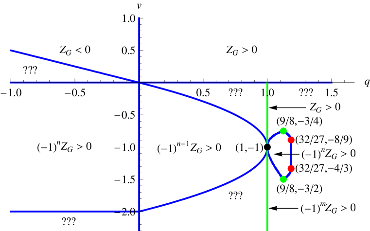
Figure 1: Sign of $Z_{G}(q,{\bf v})$ for (loopless) 2-connected graphs $G$. The cases $q>0$, $v\geq 0$ and $q=1$ are trivial (see Section 3). The remaining cases $q<0$, $0<q<1$ and $1<q\leq 32/27$ are proven in Sections 4, 5 and 9, respectively.

One message of the present paper (see also [31]) is that there is considerable advantage in studying the multivariate polynomial $Z_{G}(q,{\bf v})$, even if one is ultimately interested in a particular two-variable or one-variable specialization. For instance, $Z_{G}(q,{\bf v})$ is multiaffine in the variables ${\bf v}$ (i.e., of degree 1 in each $v_{e}$ separately); and often a multiaffine polynomial in many variables is easier to handle than a general polynomial in a single variable (e.g., it may permit simple proofs by induction on the number of variables). Furthermore, many natural operations on graphs, such as the reduction of edges in series or parallel, lead out of the class of “all $v_{e}$ equal”. For these reasons, the multivariate extension of a single-variable result is sometimes much easier to prove than its single-variable specialization. Examples of the advantage obtained by considering general $\{v_{e}\}$ are:

• a simple proof of the Brown–Hickman theorem on chromatic roots of large subdivisions (compare [30, Appendix A] with [2]);

• a very simple proof of the (multivariate) Brown–Colbourn conjecture on the zeros of reliability polynomials, in the special case of series-parallel graphs (compare [29, Remark 3 in Section 4.1] with [35]); and

• a disproof of the Brown–Colbourn conjecture for general graphs [25]. (Both the univariate and multivariate conjectures are false for general graphs; but a counterexample to the univariate conjecture would have been very difficult to find by direct search. Rather, one first shows that the complete graph $K_{4}$ is a counterexample to the multivariate conjecture; one then uses the formulae for parallel connection of edges to find a 16-edge counterexample to the univariate conjecture.)

In this paper we shall give further examples of the utility of considering general $\{v_{e}\}$; in particular, we shall elucidate the origin of the curious number 32/27 in Theorem 1.1(e). A further advantage of the $Z_{G}(q,{\bf v})$ formalism is that it shows clearly the distinct roles played by the variables $q$ and $\{v_{e}\}$: namely, $q$ is a global parameter while the edge weights $\{v_{e}\}$ are variables that can be mapped.

A second message of this paper is that it is sometimes advantageous to “think matroidal”, even when the ultimate goal is to study graphs. Indeed, as Oxley [21] has eloquently shown, graph theorems can often be improved by rethinking them in matroidal terms — that is, by eliminating reference to concepts that have no matroidal analogue (e.g. vertices and their degrees, connected components, …) and replacing them by matroidal concepts (e.g. rank, circuits, cocircuits, …). Another advantage of working with matroids is that every matroid has a dual, while only planar graphs have duals with reasonable algebraic properties. The matroidal philosophy is particularly pertinent in the present case, because the multivariate Tutte polynomial can be defined naturally for matroids (Section 2.1) and even in the graphical case it “sees” only the underlying matroidal structure (that is, two graphs with the same cycle matroid have the same multivariate Tutte polynomial, modulo trivial factors of $q$). For this reason, we believe that matroids are the “natural” category for studying the multivariate Tutte polynomial.

The plan of this paper is as follows: In Section 2 we review the definition of the multivariate Tutte polynomial for graphs and matroids, along with some of its elementary properties. In Section 3 we briefly discuss the trivial cases $q>0$, $v\geq 0$ and $q=1$. In Sections 4 and 5 we study the intervals $q<0$ and $0<q<1$, respectively. In Section 6 we prove an abstract result that will be important in what follows. In Section 7 we strengthen the results for $0<q<1$ by considering the block structure of $G$. In Section 8 we collect some properties of the “diamond map”, which plays a fundamental role in our analysis. In Section 9 we study the interval $1<q\leq 32/27$. Finally, in Section 10 we state some conjectured extensions of our results.

Since some readers of this paper may be unfamiliar with matroids, we shall ordinarily state and prove each theorem first for graphs and only afterwards for matroids, even though logically speaking the latter contains the former. In most cases the matroidal proofs will be nearly direct translations of the graphical proofs into matroidal language; we shall therefore usually be brief in discussing the matroidal proofs, drawing attention only to any non-obvious points.

2 The multivariate Tutte polynomial

2.1 Definition for graphs and matroids

Let $G=(V,E)$ be a finite undirected graph with vertex set $V$ and edge set $E$; in this paper all graphs are allowed to have loops and multiple edges unless explicitly stated otherwise. The multivariate Tutte polynomial of $G$ is, by definition, the polynomial

$$Z_{G}(q,{\bf v})\;=\;\sum_{A\subseteq E}q^{k(A)}\prod_{e\in A}v_{e}\;,$$ (2.1)

where $q$ and ${\bf v}=\{v_{e}\}_{e\in E}$ are commuting indeterminates, and $k(A)$ denotes the number of connected components in the subgraph $(V,A)$. [It is sometimes convenient to consider instead

$$\widetilde{Z}_{G}(q,{\bf v})\;\equiv\;q^{-|V|}Z_{G}(q,{\bf v})\;=\;\sum_{A\subseteq E}q^{k(A)-|V|}\prod_{e\in A}v_{e}\;,$$ (2.2)

which is a polynomial in $q^{-1}$ and $\{v_{e}\}$.] From a combinatorial point of view, $Z_{G}$ is simply the multivariate generating polynomial that enumerates the spanning subgraphs of $G$ according to their precise edge content (with weight $v_{e}$ for the edge $e$) and their number of connected components (with weight $q$ for each component). As we shall see, $Z_{G}$ encodes a vast amount of combinatorial information about the graph $G$, and contains many other well-known graph polynomials as special cases. In this paper we shall take an analytic point of view, and treat $q$ and $\{v_{e}\}$ as real variables.

If we set all the edge weights $v_{e}$ equal to the same value $v$, we obtain a two-variable polynomial $Z_{G}(q,v)$ that is equivalent to the standard Tutte polynomial $T_{G}(x,y)$ after a simple change of variables [see (2.17) below].

All of these considerations can be extended from graphs to matroids. Let $M$ be a matroid with ground set $E$ and rank function $r_{M}\colon\,2^{E}\to{\mathbb{N}}$. We then define the multivariate Tutte polynomial

$$\widetilde{Z}_{M}({q,{\bf v}})\;=\;\sum_{A\subseteq E}q^{-r_{M}(A)}\prod_{e\in A}v_{e}\;,$$ (2.3)

which is a polynomial in $q^{-1}$ and $\{v_{e}\}$. This extends the graph definition (2.2) in the sense that if $G$ is a graph and $M(G)$ is its cycle matroid, then

$$\widetilde{Z}_{M(G)}(q,{\bf v})\;=\;\widetilde{Z}_{G}(q,{\bf v})$$ (2.4)

[because $r_{M(G)}(A)=|V|-k(A)$]. Since a matroid is completely determined by its rank function, $\widetilde{Z}_{M}$ is simply an algebraic encoding of all the information about the matroid $M$. Moreover, our earlier statement that $Z_{G}$ encodes “a vast amount” of information about the graph $G$ can now be made more precise: $Z_{G}$ encodes the number of vertices $|V|$ together with all the information about $G$ that is contained in its cycle matroid $M(G)$ [and no other information]. In particular, if $G$ is loopless and 3-connected, then it is uniquely determined (within the class of loopless graphs without isolated vertices) by its cycle matroid $M(G)$ and hence by $\widetilde{Z}_{G}$ (or equivalently by $Z_{G}$); this is a special case of Whitney’s 2-isomorphism theorem [20, Theorem 5.3.1 and Lemma 5.3.2].

Let us also remark [31] that the multivariate Tutte polynomial of a matroid $M$ is related to that of its dual matroid $M^{*}$ by the formula

$$\widetilde{Z}_{M^{*}}(q,{\bf v})&=q^{-r_{M^{*}}(E)}\left(\prod\limits_{e\in E}v_{e}\right)\widetilde{Z}_{M}(q,q/{\bf v})\\ =q^{r_{M}(E)}\left(\prod\limits_{e\in E}{v_{e}\over q}\right)\widetilde{Z}_{M}(q,q/{\bf v})\;.$$ (2.5)

(Here $q/{\bf v}=\{q/v_{e}\}_{e\in E}$, $r_{M}(E)$ is the rank of $M$, $r_{M^{*}}(E)$ is the rank of $M^{*}$, and we have $r_{M}(E)+r_{M^{*}}(E)=|E|$.) In brief, duality takes $v_{e}\mapsto q/v_{e}$ (and inserts some prefactors). Indeed, the duality formula (2.5) is an easy consequence of the definition (2.3) together with the formula for the rank function of a dual:

$$r_{M^{*}}(A)\;=\;|A|\,+\,r_{M}(E\setminus A)\,-\,r_{M}(E)\;.$$ (2.6)

It goes without saying that the duality formula (2.5) can be specialized from matroids to planar graphs. One of the advantages of working with matroids is that we can think about duality even for non-planar graphs.

It is convenient to introduce explicitly the coefficients of $Z_{G}({q,{\bf v}})$ as a polynomial in $q$:

$$Z_{G}({q,{\bf v}})\;=\;\sum\limits_{k=1}^{n}C_{G}^{[k]}({\bf v})\,q^{k}$$ (2.7)

where $n=|V|$ and

$$C_{G}^{[k]}({\bf v})\;=\;\sum\limits_{00112233\begin{array}[]{c}A\subseteq E\\ k(A)=k\end{array}}\prod_{e\in A}v_{e}\;.$$ (2.8)

Likewise, let us introduce the coefficients of $\widetilde{Z}_{M}({q,{\bf v}})$ as a polynomial in $q^{-1}$:

$$\widetilde{Z}_{M}({q,{\bf v}})\;=\;\sum\limits_{r=0}^{r(M)}\widetilde{C}_{M}^{[r]}({\bf v})\,q^{-r}$$ (2.9)

where

$$\widetilde{C}_{M}^{[r]}({\bf v})\;=\;\sum\limits_{00112233\begin{array}[]{c}A\subseteq E\\ r_{M}(A)=r\end{array}}\prod_{e\in A}v_{e}\;.$$ (2.10)

2.2 Coloring interpretation for graphs

Let $G=(V,E)$ be a finite graph and let $q$ be a positive integer. A proper $q$-coloring of $G$ is a map $\sigma\colon\,V\to\{1,2,\ldots,q\}$ such that $\sigma(i)\neq\sigma(j)$ for all pairs of adjacent vertices $i,j$. It is not hard to show (see below) that for each graph $G$ there exists a polynomial $P_{G}(q)$ with integer coefficients such that, for each $q\in{\mathbb{Z}}_{+}$, the number of proper $q$-colorings of $G$ is precisely $P_{G}(q)$. This (obviously unique) polynomial $P_{G}(q)$ is called the chromatic polynomial of $G$.

A more general polynomial can be obtained as follows: Assign to each edge $e\in E$ a real or complex weight $v_{e}$, and write ${\bf v}=\{v_{e}\}_{e\in E}$ for the collection of these weights. Then the $q$-state Potts-model partition function for the graph $G$ is defined by

$$Z_{G}^{\rm Potts}({q,{\bf v}})\;=\;\sum_{\sigma\colon\,V\to\{1,2,\ldots,q\}}\;\prod_{e\in E}\,\biggl{[}1+v_{e}\delta(\sigma_{x_{1}(e)},\sigma_{x_{2}(e)})\biggr{]}\;.$$ (2.11)

Here the sum runs over all maps $\sigma\colon\,V\to\{1,2,\ldots,q\}$, and we sometimes write $\sigma_{x}$ as a synonym for $\sigma(x)$; the $\delta$ is the Kronecker delta

$$\delta(a,b)\;=\;\cases{1&if $a=b$\cr\vskip 2.0pt\cr 0&if $a\neq b$\cr}$$ (2.12)

and $x_{1}(e),x_{2}(e)\in V$ are the two endpoints of the edge $e$ (in arbitrary order). In particular, if we take $v_{e}=-1$ for all $e$, then a coloring $\sigma$ gets weight 1 or 0 according as it is proper or improper, so that $Z_{G}^{\rm Potts}(q,-1)$ counts the proper $q$-colorings.

In statistical physics, the formula (2.11) arises as follows: In the Potts model [22, 37, 38], an “atom” (or “spin”) at the site $x\in V$ can exist in any one of $q$ different states. A configuration is a map $\sigma\colon\,V\to\{1,\ldots,q\}$. The energy of a configuration is the sum, over all edges $e\in E$, of $0$ if the spin values at the two endpoints of that edge are unequal and $-J_{e}$ if they are equal. The Boltzmann weight of a configuration is then $e^{-\beta H}$, where $H$ is the energy of the configuration and $\beta\geq 0$ is the inverse temperature. The partition function is the sum, over all configurations, of their Boltzmann weights. Clearly this is just a rephrasing of (2.11), with $v_{e}=e^{\beta J_{e}}-1$. A parameter value $J_{e}$ (or $v_{e}$) is called ferromagnetic if $J_{e}\geq 0$ ($v_{e}\geq 0$), as it is then favored for adjacent spins to take the same value; antiferromagnetic if $-\infty\leq J_{e}\leq 0$ ($-1\leq v_{e}\leq 0$), as it is then favored for adjacent spins to take different values; and unphysical if $v_{e}\notin[-1,\infty)$, as the weights are then no longer nonnegative. The chromatic polynomial ($v_{e}=-1$) thus corresponds to the zero-temperature ($\beta\to\infty$) limit of the antiferromagnetic ($J_{e}<0$) Potts model. The main idea of the present paper is that many results for chromatic polynomials extend to part or all of the antiferromagnetic regime (and indeed into part of the unphysical regime as well).

It is far from obvious that $Z_{G}^{\rm Potts}({q,{\bf v}})$, which is defined separately for each positive integer $q$, is in fact the restriction to $q\in{\mathbb{Z}}_{+}$ of a polynomial in $q$. But this is in fact the case, and indeed we have:

Theorem 2.1 (Fortuin–Kasteleyn [17, 11] representation of the Potts model)

For integer $q\geq 1$,

$$Z_{G}^{\rm Potts}({q,{\bf v}})\;=\;Z_{G}(q,{\bf v})\;.$$ (2.13)

That is, the Potts-model partition function is simply the specialization of the multivariate Tutte polynomial to $q\in{\mathbb{Z}}_{+}$.

Proof. In (2.11), expand out the product over $e\in E$, and let $A\subseteq E$ be the set of edges for which the term $v_{e}\delta(\sigma_{x_{1}(e)},\sigma_{x_{2}(e)})$ is taken. Now perform the sum over configurations $\{\sigma_{x}\}_{x\in V}$: in each component of the subgraph $(V,A)$ the color $\sigma_{x}$ must be constant, and there are no other constraints. Therefore,

$$Z^{\rm Potts}_{G}({q,{\bf v}})\;=\;\sum_{A\subseteq E}q^{k(A)}\prod_{e\in A}v_{e}\;,$$ (2.14)

as was to be proved.  $\Box$

The subgraph expansion (2.14) was discovered by Birkhoff [1] and Whitney [36] for the special case $v_{e}=-1$ (see also Tutte [33, 34]); in its general form it is due to Fortuin and Kasteleyn [17, 11] (see also [9]).

Special cases of the multivariate Tutte polynomial $Z_{G}({q,{\bf v}})$ include the chromatic polynomial ($v=-1$) and the flow polynomial ($v=-q$), and more generally the standard two-variable Tutte polynomial. Indeed, we have

$$P_{G}(q) = Z_{G}(q,-1)$$ (2.15)

$$F_{G}(q) = q^{-|V|}(-1)^{|E|}Z_{G}(q,-q)$$ (2.16)

$$T_{G}(x,y) = (x-1)^{-k(E)}\,(y-1)^{-|V|}\,Z_{G}\Bigl{(}(x-1)(y-1),\,y-1\Bigr{)}\;.$$ (2.17)

Several other evaluations of the multivariate Tutte polynomial are discussed in [31].

2.3 Elementary identities

We now wish to prove some elementary identities for the multivariate Tutte polynomial. There are two alternative approaches to proving such identities: one is to prove the identity directly for real or complex $q$ (or considering $q$ as an algebraic indeterminate), using the subgraph expansion (2.1) or its generalization (2.3) to matroids; the other is to prove the identity first for positive integer $q$, using the coloring representation (2.11)/(2.13), and then to extend it to general $q$ by arguing that two polynomials (or rational functions) that coincide at infinitely many points must be equal. The latter approach is perhaps less elegant, but it is often simpler or more intuitive. However, only the former approach extends to arbitrary matroids.

One way to guess (albeit not to prove) an identity for matroids is to prove it first for graphs, and then translate it from $Z_{G}$ to $\widetilde{Z}_{G}=q^{-|V|}Z_{G}$; usually the latter identity carries over verbatim to matroids, mutatis mutandis.

In this paper we shall use four principal tools: factorization over blocks, the deletion-contraction identity, the parallel-reduction identity, and the series-reduction identity.

Factorization. If $G$ is the disjoint union of $G_{1}$ and $G_{2}$, then trivially

$$Z_{G}(q,{\bf v})\;=\;Z_{G_{1}}(q,{\bf v})\,Z_{G_{2}}(q,{\bf v})\;.$$ (2.18)

That is, $Z_{G}$ “factorizes over components”.

A slightly less trivial situation arises when $G$ consists of subgraphs $G_{1}$ and $G_{2}$ joined at a single cut vertex $x$; in this case

$$Z_{G}(q,{\bf v})\;=\;{Z_{G_{1}}(q,{\bf v})\,Z_{G_{2}}(q,{\bf v})\over q}\;.$$ (2.19)

This is easily seen from the subgraph expansion in the variant form

$$Z_{G}(q,{\bf v})\;=\;q^{|V|}\,\sum_{A\subseteq E}q^{\gamma(A)}\prod_{e\in A}{v_{e}\over q}\;,$$ (2.20)

where

$$\gamma(A)\;=\;k(A)\,-\,|V|\,+\,|A|$$ (2.21)

is the cyclomatic number (i.e., number of linearly independent cycles) of the graph $(V,A)$. It is also easily seen from the coloring representation (2.11)/(2.13) by first fixing the color $\sigma_{x}$ at the cut vertex and then summing over it; from this viewpoint, (2.19) reflects the $S_{q}$ permutation symmetry of the $q$-state Potts model. We summarize (2.19) by saying that $Z_{G}$ “factorizes over blocks” modulo a factor $q$.

The identities (2.18) and (2.19) can be written in a unified form, by using $\widetilde{Z}_{G}=q^{-|V|}Z_{G}$: in both cases we have

$$\widetilde{Z}_{G}(q,{\bf v})\;=\;\widetilde{Z}_{G_{1}}(q,{\bf v})\,\widetilde{Z}_{G_{2}}(q,{\bf v})\;.$$ (2.22)

This, in turn, is a special case of the following obvious fact: if a matroid $M$ is the direct sum of matroids $M_{1}$ and $M_{2}$, then

$$\widetilde{Z}_{M}(q,{\bf v})\;=\;\widetilde{Z}_{M_{1}}(q,{\bf v})\,\widetilde{Z}_{M_{2}}(q,{\bf v})\;.$$ (2.23)

Deletion-contraction identity. If $e\in E$, let $G\setminus e$ denote the graph obtained from $G$ by deleting the edge $e$, and let $G/e$ denote the graph obtained from $G\setminus e$ by contracting the two endpoints of $e$ into a single vertex (please note that we retain in $G/e$ any loops or multiple edges that may be formed as a result of the contraction). Then, for any $e\in E$, we have the identity

$$Z_{G}({q,{\bf v}})\;=\;Z_{G\setminus e}(q,{\bf v}_{\neq e})\,+\,v_{e}Z_{G/e}(q,{\bf v}_{\neq e})\;.$$ (2.24)

This is easily seen either from the coloring representation (2.11)/(2.13) or the subgraph expansion (2.1). Please note that the deletion-contraction identity (2.24) takes the same form regardless of whether $e$ is a normal edge, a loop, or a bridge (in contrast to the situation for the usual Tutte polynomial $T_{G}$). Of course, if $e$ is a loop, then $G/e=G\setminus e$, so we can also write

$$Z_{G}\;=\;(1+v_{e})Z_{G\setminus e}\;=\;(1+v_{e})Z_{G/e}\qquad\hbox{if $e$ is a loop}\;.$$ (2.25)

Similarly, if $e$ is a bridge, then $G\setminus e$ is the disjoint union of two subgraphs $G_{1}$ and $G_{2}$ while $G/e$ is obtained by joining $G_{1}$ and $G_{2}$ at a cut vertex, so that $Z_{G/e}=Z_{G\setminus e}/q$ and hence

$$Z_{G}\;=\;(1+v_{e}/q)Z_{G\setminus e}\;=\;(q+v_{e})Z_{G/e}\qquad\hbox{if $e$ is a bridge}\;.$$ (2.26)

The deletion-contraction identity applies also to the coefficients $C_{G}^{[k]}$ of the multivariate Tutte polynomial:

$$C_{G}^{[k]}({\bf v})\;=\;C_{G\setminus e}^{[k]}({\bf v}_{\neq e})\,+\,v_{e}C_{G/e}^{[k]}({\bf v}_{\neq e})\;.$$ (2.27)

This follows either by examining the definition (2.8) or by observing that the deletion-contraction identity (2.24) for $Z_{G}$ does not mix powers of $q$.

In terms of $\widetilde{Z}_{G}=q^{-|V|}Z_{G}$, the deletion-contraction identity takes the form

$$\widetilde{Z}_{G}&=\widetilde{Z}_{G\setminus e}\,+\,{v_{e}\over q}\widetilde{Z}_{G/e}\qquad\hbox{if $e$ is not a loop}\\ \widetilde{Z}_{G}=\widetilde{Z}_{G\setminus e}\,+\,v_{e}\widetilde{Z}_{G/e}\\ =(1+v_{e})\widetilde{Z}_{G\setminus e}\\ =(1+v_{e})\widetilde{Z}_{G/e}\qquad\quad\;\hbox{if $e$ is a loop}$$ (2.28)

as easily follows from (2.24) together with the counting of vertices in $G\setminus e$ and $G/e$.

Not surprisingly, the deletion-contraction formula for matroids is identical in form to (2.28):

$$\widetilde{Z}_{M}&=\widetilde{Z}_{M\setminus e}\,+\,{v_{e}\over q}\widetilde{Z}_{M/e}\qquad\hbox{if $e$ is not a loop}\\ \widetilde{Z}_{M}=\widetilde{Z}_{M\setminus e}\,+\,v_{e}\widetilde{Z}_{M/e}\\ =(1+v_{e})\widetilde{Z}_{M\setminus e}\\ =(1+v_{e})\widetilde{Z}_{M/e}\qquad\quad\;\hbox{if $e$ is a loop}$$ (2.29)

This easily follows from the formulae for the rank function of a deletion or contraction: if $A\subseteq E\setminus e$, then

$$r_{M\setminus e}(A)&=r_{M}(A)\\ r_{M/e}(A)=\cases{r_{M}(A\cup e)-1&if $e$ is not a loop\cr r_{M}(A\cup e)&if $e$ is a loop\cr}{}$$ (2.30)

Parallel-reduction identity. If $G$ contains edges $e_{1},e_{2}$ connecting the same pair of vertices $x,y$, they can be replaced, without changing the value of $Z$, by a single edge $e=xy$ with weight

$$v_{e}\;=\;(1+v_{e_{1}})(1+v_{e_{2}})\,-\,1\;=\;v_{e_{1}}+v_{e_{2}}+v_{e_{1}}v_{e_{2}}\;.$$ (2.31)

This is easily seen either from the coloring representation (2.11)/(2.13) or the subgraph expansion (2.1). More formally, we can write

$$Z_{G}(q,{\bf v}_{\neq e_{1},e_{2}},v_{e_{1}},v_{e_{2}})\;=\;Z_{G\setminus e_{2}}(q,{\bf v}_{\neq e_{1},e_{2}},v_{e_{1}}+v_{e_{2}}+v_{e_{1}}v_{e_{2}})\;.$$ (2.32)

The parallel-reduction rule $(v_{1},v_{2})\mapsto v_{\rm eff}$ with $1+v_{\rm eff}=(1+v_{1})(1+v_{2})$ can be remembered by the mnemonic “$1+v$ multiplies”. We write $v_{1}\|v_{2}\equiv(1+v_{1})(1+v_{2})-1$; and if ${\mathcal{V}}_{1},{\mathcal{V}}_{2}\subseteq{\mathbb{R}}$ (or ${\mathbb{C}}$) we write ${\mathcal{V}}_{1}\|{\mathcal{V}}_{2}\equiv\{v_{1}\|v_{2}\colon\,v_{1}\in{\mathcal{V}}_{1},\,v_{2}\in{\mathcal{V}}_{2}\}$.

The parallel-reduction rule applies also to the $C_{G}^{[k]}$:

$$C_{G}^{[k]}({\bf v}_{\neq e_{1},e_{2}},v_{e_{1}},v_{e_{2}})\;=\;C_{G\setminus e_{2}}^{[k]}({\bf v}_{\neq e_{1},e_{2}},v_{e_{1}}+v_{e_{2}}+v_{e_{1}}v_{e_{2}})\;.$$ (2.33)

This follows either from the definition (2.8) or by observing that the parallel-reduction rule for $Z_{G}$ does not mix powers of $q$.

A virtually identical formula holds for matroids: if $e_{1}$ and $e_{2}$ are parallel elements in a matroid $M$ (i.e., form a two-element circuit), then

$$\widetilde{Z}_{M}(q,{\bf v}_{\neq e_{1},e_{2}},v_{e_{1}},v_{e_{2}})\;=\;\widetilde{Z}_{M\setminus e_{2}}(q,{\bf v}_{\neq e_{1},e_{2}},v_{e_{1}}+v_{e_{2}}+v_{e_{1}}v_{e_{2}})\;.$$ (2.34)

The formula (2.34) also holds trivially if $e_{1}$ and $e_{2}$ are both loops.

Series-reduction identity. We say that edges $e_{1},e_{2}\in E$ are in series (in the narrow sense) if there exist vertices $x,y,z\in V$ with $x\neq y$ and $y\neq z$ such that $e_{1}$ connects $x$ and $y$, $e_{2}$ connects $y$ and $z$, and $y$ has degree 2 in $G$. In this case the pair of edges $e_{1},e_{2}$ can be replaced, without changing the value of $Z$, by a single edge $e=xz$ with weight

$$v_{e}\;=\;{v_{e_{1}}v_{e_{2}}\over q+v_{e_{1}}+v_{e_{2}}}$$ (2.35)

provided that we then multiply $Z$ by the prefactor $q+v_{e_{1}}+v_{e_{2}}$. More formally, we can write

$$Z_{G}(q,{\bf v}_{\neq e_{1},e_{2}},v_{e_{1}},v_{e_{2}})\;=\;(q+v_{e_{1}}+v_{e_{2}})\,Z_{G/e_{2}}(q,{\bf v}_{\neq e_{1},e_{2}},v_{e_{1}}v_{e_{2}}/(q+v_{e_{1}}+v_{e_{2}}))\;.$$ (2.36)

This identity can be derived from the coloring representation (2.11)/(2.13) by noting that

$$\sum_{\sigma_{y}=1}^{q}[1+v_{e_{1}}\delta(\sigma_{x},\sigma_{y})][1+v_{e_{2}}\delta(\sigma_{y},\sigma_{z})]&=q+v_{e_{1}}+v_{e_{2}}+v_{e_{1}}v_{e_{2}}\delta(\sigma_{x},\sigma_{z})\\ =(q+v_{e_{1}}+v_{e_{2}})\left[1\,+\,{v_{e_{1}}v_{e_{2}}\over q+v_{e_{1}}+v_{e_{2}}}\delta(\sigma_{x},\sigma_{z})\right]\;.\\$$ (2.37)

Alternatively, it can be derived from the subgraph expansion (2.1) by considering the four possibilities for the edges $e_{1}$ and $e_{2}$ to be occupied or empty and analyzing the number of connected components thereby created. The series-reduction rule $(v_{1},v_{2})\mapsto v_{\rm eff}\equiv v_{1}v_{2}/(q+v_{1}+v_{2})$ can be remembered by the mnemonic “$1+q/v$ multiplies”: namely,

$$1+{q\over v_{\rm eff}}\;=\;\left(1+{q\over v_{1}}\right)\left(1+{q\over v_{2}}\right)\;.$$ (2.38)

We write $v_{1}{\,\bowtie_{q}\,}v_{2}\equiv v_{1}v_{2}/(q+v_{1}+v_{2})$; and if ${\mathcal{V}}_{1},{\mathcal{V}}_{2}\subseteq{\mathbb{R}}$ (or ${\mathbb{C}}$) we write ${\mathcal{V}}_{1}{\,\bowtie_{q}\,}{\mathcal{V}}_{2}\equiv\{v_{1}{\,\bowtie_{q}\,}v_{2}\colon\,v_{1}\in{\mathcal{V}}_{1},\,v_{2}\in{\mathcal{V}}_{2}\}$.

Consider now the more general situation in which $\{e_{1},e_{2}\}$ is a two-edge cut of $G$ (not necessarily the cut associated with a degree-2 vertex $y$); we then say that $e_{1},e_{2}$ are in series (in the wide sense). It turns out that the identity (2.36) still holds. To see this, let us prove the generalization of this identity to matroids. Let $e_{1}$ and $e_{2}$ be series elements in a matroid $M$, i.e., suppose that $\{e_{1},e_{2}\}$ is a cocircuit. Then, for any $A\subseteq E\setminus\{e_{1},e_{2}\}$, we have

$$r_{M}(A\cup e_{1})\;=\;r_{M}(A\cup e_{2})\;=\;r_{M}(A)+1$$ (2.39)

(since the complement of a cocircuit is a hyperplane). A short calculation using (LABEL:eq.rank.contraction) with $e=e_{2}$ then yields

$$\widetilde{Z}_{M}(q,{\bf v}_{\neq e_{1},e_{2}},v_{e_{1}},v_{e_{2}})\;=\;{q+v_{e_{1}}+v_{e_{2}}\over q}\,\widetilde{Z}_{M/e_{2}}(q,{\bf v}_{\neq e_{1},e_{2}},v_{e_{1}}v_{e_{2}}/(q+v_{e_{1}}+v_{e_{2}}))\;.$$ (2.40)

The formula (2.40) also holds trivially if $e_{1}$ and $e_{2}$ are both coloops.

Please note that duality $v\mapsto q/v$ interchanges the parallel-reduction rule (“$1+v$ multiplies”) with the series-reduction rule (“$1+q/v$ multiplies”). This is no accident, since we now see that parallel-reduction and series-reduction (in the wide sense) are indeed duals of each other: $\{e_{1},e_{2}\}$ is a circuit (resp. cocircuit) in $M$ if and only if it is a cocircuit (resp. circuit) in the dual matroid $M^{*}$.

3 Two trivial cases

Let us begin by disposing of two cases in which we can trivially control the sign of $Z_{G}(q,{\bf v})$.

Proposition 3.1

Let $G$ be a graph with $n$ vertices, and suppose that $v_{e}\geq 0$ for all $e$. Then $Z_{G}(q,{\bf v})\geq q^{n}>0$ for $q>0$; and more generally, for $0\leq\ell\leq n$ we have

$${d^{\ell}\over dq^{\ell}}\,Z_{G}(q,{\bf v})\;\geq\;n^{\underline{\ell}}q^{n-\ell}\;>\;0\qquad\hbox{for }q>0$$ (3.1)

[here $n^{\underline{\ell}}=n(n-1)\cdots(n-\ell+1)$].

Proof. In the definition (2.1), the term $A=\varnothing$ contributes $q^{n}$, and the remaining terms contribute a polynomial in $q$ with nonnegative coefficients.  $\Box$

A similar result holds for matroids, but since $\widetilde{Z}_{M}({q,{\bf v}})$ involves inverse powers of $q$ [cf. (2.3)], we can no longer control the derivatives with respect to $q$:

Proposition 3.2

Let $M$ be a matroid, and suppose that $v_{e}\geq 0$ for all $e$. Then $\widetilde{Z}_{M}(q,{\bf v})\geq 1>0$ for $q>0$.

The other trivial case is $q=1$, because $Z_{G}(1,{\bf v})=\prod\limits_{e\in E}(1+v_{e})$ and more generally $\widetilde{Z}_{M}({q,{\bf v}})=\prod\limits_{e\in E}(1+v_{e})$. It follows that:

Proposition 3.3

Let $G$ be a graph with $m$ edges.

• If $v_{e}>-1$ for all $e$, then $Z_{G}(1,{\bf v})>0$.

• If $v_{e}<-1$ for all $e$, then $(-1)^{m}Z_{G}(1,{\bf v})>0$.

The corresponding result of course holds for a matroid on a ground set with $m$ elements.

4 The interval $q\in(-\infty,0)$

It is well known that the coefficients of the chromatic polynomial alternate in sign, and the leading coefficient is 1 whenever the graph is loopless. These facts immediately imply that $P_{G}(q)$ is nonzero with sign $(-1)^{n}$ for $q<0$. The following theorem generalizes this result to the multivariate Tutte polynomial $Z_{G}({q,{\bf v}})$:

Theorem 4.1

Let $G$ be a graph with $n$ vertices and $c$ components. Suppose that

• $v_{e}\geq-1$ for every loop $e$; and

• $-2\leq v_{e}\leq 0$ for every non-loop edge $e$.

Then:

• $C_{G}^{[k]}\equiv 0$ for $1\leq k<c$, $(-1)^{n-k}C_{G}^{[k]}({\bf v})\geq 0$ for $c\leq k\leq n$, and
  $C_{G}^{[n]}=\prod\limits_{{\rm loops}\,e}(1+v_{e})$.

• $(-1)^{n}Z_{G}({q,{\bf v}})\geq 0$ for all $q<0$, with strict inequality if and only if every loop has $v_{e}>-1$.

Furthermore, if

• $v_{e}>-1$ for every loop $e$; and

• $-2<v_{e}<0$ for every non-loop edge $e$,

then:

• $(-1)^{n-k}C_{G}^{[k]}({\bf v})>0$ for $c\leq k\leq n$.

• The root of $Z_{G}({q,{\bf v}})$ at $q=0$ has multiplicity $c$.

Please note that Theorem 1.1(a,b) are the special cases of Theorem 4.1(b,b^′) in which the graph is loopless and $v_{e}=-1$ for all edges $e$. We now see that these results can be generalized to $v_{e}\in[-2,0]$ and $v_{e}\in(-2,0)$, respectively. In particular, Theorem 1.1(a,b) extends to the whole antiferromagnetic regime $[-1,0]$ as well as to part of the unphysical regime $(-\infty,-1]$.

Let us also remark that since $q<0$, conclusion (b) can equivalently be written as $\widetilde{Z}_{G}({q,{\bf v}})\geq 0$. This way of writing Theorem 4.1 also suggests that the correct generalization to matroids will be $\widetilde{Z}_{M}({q,{\bf v}})\geq 0$: see Theorem 4.3 below.

Proof of Theorem 4.1.  It suffices to prove (a), since (b) is then an immediate corollary. Since each loop $e$ simply contributes an overall factor $1+v_{e}$, which has the right sign by hypothesis, we can assume henceforth that $G$ is loopless. By (2.8), $C_{G}^{[k]}\equiv 0$ for $1\leq k<c$ and, since $G$ is loopless, $C_{G}^{[n]}\equiv 1$. The proof of the sign inequalities for $C_{G}^{[k]}$ is by induction on the number of edges in $G$. If $G$ has no edges, then $c=n$ and (a) holds. Now suppose that $G$ has $m$ edges, and assume that the result holds for all graphs having fewer than $m$ edges. We now consider three cases:

(i) If $G$ is a forest, then we have $k(A)=n-|A|$ for every $A\subseteq E$, so that

$$C_{G}^{[k]}({\bf v})\;=\;\sum\limits_{00112233\begin{array}[]{c}A\subseteq E\\ |A|=n-k\end{array}}\prod_{e\in A}v_{e}\;.$$ (4.1)

Since $v_{e}\leq 0$ for all $e$, statement (a) holds.

We can henceforth suppose that $G$ has at least one circuit.

(ii) If $G$ has somewhere a pair $e_{1},e_{2}$ of parallel edges, pick some such pair and apply the parallel-reduction formula (2.33) to it. Since $(v_{1},v_{2})\mapsto(1+v_{1})(1+v_{2})-1$ maps the interval $[-2,0]$ into itself, we can apply the inductive hypothesis to $G\setminus e_{2}$; and the result has the right sign, since $G\setminus e_{2}$ has the same number of vertices and components as $G$ does.

(iii) If $G$ has no pair of parallel edges, pick any edge $e$ which belongs to a circuit of $G$ and apply the deletion-contraction identity (2.27). By the inductive hypothesis, the first term has the right sign, since $G\setminus e$ has the same number of vertices and components as $G$ does. Since $G$ has no parallel edges, $G/e$ is loopless, so we can apply the inductive hypothesis to it as well; moreover, since $e$ is not a loop, $G/e$ has one vertex fewer than $G$ and the same number of components as $G$; therefore, since $v_{e}\leq 0$, the second term has the right sign as well.

This proves (a); and the same argument, with minor modifications, proves (a^′) under the hypotheses (i^′) and (ii^′). Statement (b^′) then follows from $C_{G}^{[k]}=0$ for $k<c$ and $C_{G}^{[k]}\neq 0$ for $k=c$.  $\Box$

The interval $[-2,0]$ is best possible, as is shown by the following example:

Example 4.1.  Let $G=K_{2}^{(m)}$ (a single pair of vertices connected by $m$ parallel edges). Then $Z_{G}(q,v)=q[q+(1+v)^{m}-1]$, so that for any $q<0$ there are roots $v$ tending to $-2$ (from below) and to $0$ (from above) as $m\to\infty$ (the former only for $m$ even).  $\Box$

We can also prove some inequalities on the partial derivatives of $C_{G}^{[k]}({\bf v})$ with respect to individual weights $v_{e}$, provided that we make a slightly stronger hypothesis on the interval in which the weights $v_{e}$ lie. If $e_{1},\ldots,e_{\ell}$ are edges in $G$ and $e\in E\setminus\{e_{1},\ldots,e_{\ell}\}$, let us say that $e$ is spanned by $\{e_{1},\ldots,e_{\ell}\}$ if there exists a subset of $\{e_{1},\ldots,e_{\ell}\}$ which together with $e$ forms a circuit [or equivalently, if $\{e_{1},\ldots,e_{\ell}\}\cup\{e\}$ has a cyclomatic number larger than that of $\{e_{1},\ldots,e_{\ell}\}$; or equivalently, if the rank of $\{e_{1},\ldots,e_{\ell}\}\cup\{e\}$ in the cycle matroid $M(G)$ is equal to that of $\{e_{1},\ldots,e_{\ell}\}$]. Note that a loop is spanned by any set of edges (even the empty set).

Corollary 4.2

Let $G=(V,E)$ be a graph with $n$ vertices, and let $\ell\geq 0$ and $e_{1},\ldots,e_{\ell}\in E$. Suppose that

• $-2\leq v_{e}\leq 0$ for all $e\in E\setminus\{e_{1},\ldots,e_{\ell}\}$ that are not spanned by $\{e_{1},\ldots,e_{\ell}\}$; and

• $v_{e}\geq-1$ for all $e\in E\setminus\{e_{1},\ldots,e_{\ell}\}$ that are spanned by $\{e_{1},\ldots,e_{\ell}\}$.

Then:

• If $e_{1},\ldots,e_{\ell}$ are not all distinct, we have

  $${\partial^{\ell}C_{G}^{[k]}({\bf v})\over\partial v_{e_{1}}\cdots\partial v_{e_{\ell}}}\;=\;0\;.$$ (4.2)

• If $e_{1},\ldots,e_{\ell}$ are all distinct and form a subgraph with cyclomatic number $\gamma$, we have

  $$(-1)^{n-k+\ell+\gamma}\,{\partial^{\ell}C_{G}^{[k]}({\bf v})\over\partial v_{e_{1}}\cdots\partial v_{e_{\ell}}}\;\geq\;0\;.$$ (4.3)

Please note that Theorem 4.1(a) is simply the special case $\ell=0$ of Corollary 4.2.

Proof. Note first that the deletion-contraction identity (2.27) implies that

$${\partial C_{G}^{[k]}({\bf v})\over\partial v_{e}}\;=\;C_{G/e}^{[k]}({\bf v}_{\neq e})$$ (4.4)

and more generally

$${\partial^{\ell}C_{G}^{[k]}({\bf v})\over\partial v_{e_{1}}\cdots\partial v_{e_{\ell}}}\;=\;C_{G/\{e_{1},\ldots,e_{\ell}\}}^{[k]}({\bf v}_{\neq e_{1},\ldots,e_{\ell}})$$ (4.5)

for any set $e_{1},\ldots,e_{\ell}$ of distinct edges. [If the edges $e_{1},\ldots,e_{\ell}$ are not distinct, then $\partial^{\ell}C_{G}^{[k]}({\bf v})/\partial v_{e_{1}}\cdots\partial v_{e_{\ell}}\equiv 0$.] Now, the graph $G/e$ has $|V|$ vertices if $e$ is a loop, and $|V|-1$ vertices if $e$ is not a loop. Iterating this fact, we see that if $e_{1},\ldots,e_{\ell}$ are distinct edges that form a subgraph with cyclomatic number $\gamma$, then $G/\{e_{1},\ldots,e_{\ell}\}$ has $|V|-\ell+\gamma$ vertices. Furthermore, if $e\in E\setminus\{e_{1},\ldots,e_{\ell}\}$, then $e$ is a loop in $G/\{e_{1},\ldots,e_{\ell}\}$ if and only if $e$ is spanned by $\{e_{1},\ldots,e_{\ell}\}$. The hypothesis $v_{e}\geq-1$ for such edges is precisely what is needed to apply Theorem 4.1. Applying (4.5) together with Theorem 4.1(a) and the foregoing observations yields (4.3).  $\Box$

Corollary 4.2 was proven a few years ago by Scott and Sokal [27, Proposition 2.7], under the slightly stronger hypothesis that $-1\leq v_{e}\leq 0$ for all $e\in E$. However, their proof used a fairly sophisticated device, namely the partitionability identity. It is nice to know that a completely elementary proof can be given, and that the conditions on $v_{e}$ can be slightly weakened.

The proof of Theorem 4.1 extends immediately to matroids, yielding:

Theorem 4.3

Let $M$ be a matroid of rank $r(M)$ on the ground set $E$. Suppose that

• $v_{e}\geq-1$ for every loop $e$; and

• $-2\leq v_{e}\leq 0$ for every non-loop edge $e$.

Then:

• $(-1)^{r}\widetilde{C}_{M}^{[r]}({\bf v})\geq 0$ for $0\leq r\leq r(M)$, with $\widetilde{C}_{M}^{[0]}=\prod\limits_{{\rm loops}\,e}(1+v_{e})$.

• $\widetilde{Z}_{M}({q,{\bf v}})\geq 0$ for all $q<0$, with strict inequality if and only if every loop has $v_{e}>-1$.

Furthermore, if

• $v_{e}>-1$ for every loop $e$; and

• $-2<v_{e}<0$ for every non-loop edge $e$,

then $(-1)^{r}\widetilde{C}_{M}^{[r]}({\bf v})>0$ for $0\leq r\leq r(M)$.

Applying Theorem 4.3 to the cographic matroid $M^{*}(G)$, we obtain a result dual to Theorem 4.1:

Theorem 4.4 (Dong [7])

Let $G$ be a graph with $c$ components, and fix $q<0$. Suppose that

• $v_{e}\geq-q$ for every bridge $e$; and

• $v_{e}\geq-q/2$ for every non-bridge edge $e$.

Then $(-1)^{c}Z_{G}({q,{\bf v}})\geq 0$, with strict inequality if and only if every bridge has $v_{e}>-q$.

This result was suggested to us by Feng-Ming Dong [7], who proved it by a direct argument that is essentially the dual of the proof of Theorem 4.1.

Similarly, the proof of Corollary 4.2 extends immediately to matroids (using the same definition of “spanned”, which is after all the matroidal one). We obtain:

Corollary 4.5

Let $M$ be a matroid of rank $r(M)$ on the ground set $E$, and let $\ell\geq 0$ and $e_{1},\ldots,e_{\ell}\in E$. Suppose that

• $-2\leq v_{e}\leq 0$ for all $e\in E\setminus\{e_{1},\ldots,e_{\ell}\}$ that are not spanned by $\{e_{1},\ldots,e_{\ell}\}$; and

• $v_{e}\geq-1$ for all $e\in E\setminus\{e_{1},\ldots,e_{\ell}\}$ that are spanned by $\{e_{1},\ldots,e_{\ell}\}$.

Then:

• If $e_{1},\ldots,e_{\ell}$ are not all distinct, we have

  $${\partial^{\ell}\widetilde{C}_{M}^{[r]}({\bf v})\over\partial v_{e_{1}}\cdots\partial v_{e_{\ell}}}\;=\;0\;.$$ (4.6)

• If $e_{1},\ldots,e_{\ell}$ are all distinct and form a set with rank $\rho$ in the matroid $M$, we have

  $$(-1)^{r+\rho}\,{\partial^{\ell}\widetilde{C}_{M}^{[r]}({\bf v})\over\partial v_{e_{1}}\cdots\partial v_{e_{\ell}}}\;\geq\;0\;.$$ (4.7)

5 The interval $q\in(0,1)$

In this section we discuss the conditions under which the sign of $Z_{G}({q,{\bf v}})$ can be controlled when $0<q<1$ and the edge weights $v_{e}$ lie in a suitable subinterval of $(-2,0)$. We prove a basic result valid for arbitrary graphs $G$ (Theorem 5.1). Later, in Section 7, we will prove a sequence of refinements that make successively stronger hypotheses on the minimum number of edges in each block of $G$, and obtain correspondingly wider intervals for the edge weights $v_{e}$.

Let $G$ be a loopless graph with $n$ vertices and $c$ components; then Theorem 1.1(c) states that $P_{G}(q)$ is nonzero with sign $(-1)^{n+c}$ for $0<q<1$. The following theorem generalizes this result to the multivariate Tutte polynomial $Z_{G}({q,{\bf v}})$:

Theorem 5.1

Let $G$ be a graph with $n$ vertices and $c$ components, and let $q\in(0,1)$. Suppose that:

• $v_{e}>-1$ for every loop $e$;

• $v_{e}<-q$ for every bridge $e$; and

• $-1-\sqrt{1-q}<v_{e}<-1+\sqrt{1-q}$ for every normal (i.e., non-loop non-bridge) edge $e$.

Then $(-1)^{n+c}Z_{G}({q,{\bf v}})>0$.

Corollary 5.2

Let $G$ be a graph with $n$ vertices and $c$ components, and let $q\in(0,1)$. Then $(-1)^{n+c}Z_{G}({q,{\bf v}})>0$ in each of the following three cases:

• $G$ is loopless, with $-1-\sqrt{1-q}<v_{e}<-q$ for all $e\in E$.

• $G$ is bridgeless, with $-1<v_{e}<-1+\sqrt{1-q}$ for all $e\in E$.

• $G$ is loopless and bridgeless, with $-1-\sqrt{1-q}<v_{e}<-1+\sqrt{1-q}$ for all $e\in E$.

Theorem 1.1(c) is the special case of Corollary 5.2(a) in which $v_{e}=-1$ for all edges $e$. We now see that this result can be extended to $v_{e}\in(-1-\sqrt{1-q},-q)$. Please note that this interval approaches $(-2,0)$ as $q\downarrow 0$, and degenerates to the empty set $(-1,-1)$ as $q\uparrow 1$.

It is worth remarking that the hypotheses of Theorem 5.1 and Corollary 5.2 are invariant under duality (of planar graphs), which takes $v\mapsto q/v$ and interchanges loops and bridges. In particular, the interval $(-1-\sqrt{1-q},-1+\sqrt{1-q})$ is mapped onto itself under duality, with the endpoints interchanged.

Proof of Theorem 5.1.  The proof is by induction on the number of edges in $G$. If $G$ has no edges, then $c=n$ and $Z_{G}({q,{\bf v}})=q^{n}>0$, so the claim is obviously true. Now suppose that $G$ has $m$ edges, and assume that the result holds for all graphs having fewer than $m$ edges. We now consider five cases:

(a) If $G$ has a loop $e$, then $Z_{G}({q,{\bf v}})=(1+v_{e})Z_{G\setminus e}(q,{\bf v}_{\neq e})$ by (2.25). By hypothesis we have $1+v_{e}>0$; and $G\setminus e$ has the same numbers of components and vertices as $G$ does. This proves that $Z_{G}({q,{\bf v}})$ is nonzero with the desired sign.

(b) If $G$ has a bridge $e$, then $Z_{G}({q,{\bf v}})=(q+v_{e})Z_{G/e}(q,{\bf v}_{\neq e})$ by (2.26). By hypothesis we have $q+v_{e}<0$; and $G/e$ has the same numbers of components as $G$ but one less vertex. This proves once again that $Z_{G}({q,{\bf v}})$ is nonzero with the desired sign.

We can henceforth assume that $G$ has no loops or bridges.

(c) If $G$ has a pair $e_{1},e_{2}$ of parallel edges, then we apply the parallel-reduction formula (2.32) to it. By hypothesis, both $1+v_{1}$ and $1+v_{2}$ lie in the interval $(-\sqrt{1-q},\sqrt{1-q})$. Therefore $(1+v_{1})(1+v_{2})$ lies in the interval $(-(1-q),1-q)$, and hence $v_{\rm eff}\equiv(1+v_{1})(1+v_{2})-1$ satisfies

$$v_{\rm eff}\;\in\;\Bigl{(}-1-(1-q),\,-1+(1-q)\Bigr{)}\;\subset\;\Bigl{(}-1-\sqrt{1-q},\,-q\Bigr{)}\;.$$ (5.1)

In the graph $G\setminus e_{2}$, the edge $e_{1}$ is either a normal edge or a bridge; it cannot be a loop. The new weight (5.1) satisfies the hypotheses for both normal edges and bridges, so we may apply the inductive hypothesis to $G\setminus e_{2}$. Since $G\setminus e_{2}$ has the same number of vertices and components as $G$ does, we are done.

(d) If $G$ has a pair $e_{1},e_{2}$ of series edges in the wide sense, then we apply the series-reduction formula (2.36) to it. By hypothesis, both $1+q/v_{1}$ and $1+q/v_{2}$ lie in the interval $(-\sqrt{1-q},\sqrt{1-q})$. Therefore $(1+q/v_{1})(1+q/v_{2})$ lies in the interval $(-(1-q),1-q)$, hence

$${q\over v_{\rm eff}}\;\equiv\;\biggl{(}1+{q\over v_{1}}\biggr{)}\biggl{(}1+{q\over v_{2}}\biggr{)}\,-\,1\;\in\;(-2+q,-q)\;,$$ (5.2)

hence

$$v_{\rm eff}\;\in\;\Bigl{(}-1,\,-{q\over 2-q}\Bigr{)}\;\subset\;\Bigl{(}-1,\,-1+\sqrt{1-q}\Bigr{)}\;.$$ (5.3)

In the graph $G/e_{2}$, the edge $e_{1}$ is either a normal edge or a loop; it cannot be a bridge. The new weight (5.3) satisfies the hypotheses for both normal edges and loops, so we may apply the inductive hypothesis to $G/e_{2}$. Now, $G/e_{2}$ has the same number of components as $G$ but one less vertex. On the other hand, since $v_{1},v_{2}<-1+\sqrt{1-q}<-q/2$, the prefactor $q+v_{1}+v_{2}$ in (2.36) is negative. This gives the correct sign.

(e) If $G$ has neither parallel edges nor series edges in the wide sense, then pick any edge $e$ and apply the deletion-contraction identity (2.24) to it. We see that $G\setminus e$ has the same number of vertices and components as $G$ does (because $e$ is not a bridge); and all edges of $G\setminus e$ are normal (because $e$ does not belong to a wide-sense series pair in $G$, so a bridge cannot be formed by deletion). Therefore, we can apply the inductive hypothesis to $G\setminus e$, and the contribution has the correct sign. Likewise, we see that $G/e$ has the same number of components as $G$ but one less vertex (because $e$ is not a loop); and all edges of $G/e$ are normal (because $e$ does not belong to a parallel pair in $G$, so a loop cannot be formed by contraction). Therefore, we can apply the inductive hypothesis to $G/e$; and since $v_{e}<0$, the contribution again has the correct sign.  $\Box$

The following examples show that Theorem 5.1 and Corollary 5.2 are in some sense best possible. If $G$ is any tree, we have $Z_{G}(q,v)=q(q+v)^{n-1}$, so that there are roots at $v=-q$. If $G$ has one vertex and $k$ loops, then $Z_{G}(q,v)=(1+v)^{k}$, so that there are roots at $v=-1$. If $G$ is a cycle of length two, then we have $Z_{G}(q,v)=q(q+2v+v^{2})$, so that there are roots at $v=-1\pm\sqrt{1-q}$. We will see in Section 7, however, that Theorem 5.1 can be improved if we add a hypothesis on the minimum number of edges in a block of $G$.

We next show that, in the situation of Corollary 5.2(a), we can go farther and control derivatives with respect to $q$:

Theorem 5.3

Let $G$ be a loopless graph with $n$ vertices and $c$ components, and let $q\in(0,1)$. Suppose that $-1-\sqrt{1-q}<v_{e}<-q$ for all $e\in E$. Then for $0\leq\ell\leq n-c$ we have

$$(-1)^{n-c-\ell}\,{d^{\ell}\over dq^{\ell}}\,\biggl{(}{Z_{G}(q,{\bf v})\over q^{c}}\biggr{)}\;>\;0\;.$$ (5.4)

Proof. The proof is by induction on $|E|$. If $G$ has no edges, then $c=n$ and hence $\ell=0$; and since $Z_{G}(q,{\bf v})/q^{c}\equiv 1$, the result holds.

Now suppose that $G$ has $m$ edges, and assume that the result holds for all graphs having fewer than $m$ edges. We shall consider three cases:

(i) If $G$ is a forest, then then $Z_{G}({q,{\bf v}})/q^{c}=\prod_{e\in E}(q+v_{e})$. Since $q+v_{e}<0$ for all $e$, this product and all its derivatives have the claimed sign.

We can henceforth assume that $G$ is not a forest.

(ii) If $G$ has somewhere a pair $e_{1},e_{2}$ of parallel edges, pick some such pair and apply to it the parallel-reduction formula (2.32), differentiated $\ell$ times with respect to $q$. Since $(v_{1},v_{2})\mapsto(1+v_{1})(1+v_{2})-1$ maps the interval $(-1-\sqrt{1-q},-q)$ into itself, we can apply the inductive hypothesis to $G\setminus e_{2}$; and the result has the right sign, since $G\setminus e_{2}$ has the same number of vertices and connected components as $G$ does.

(iii) If $G$ has no pair of parallel edges, pick any non-bridge edge $e$ and apply to it the deletion-contraction identity (2.24), differentiated $\ell$ times with respect to $q$. By the inductive hypothesis, the first term has the right sign (strictly) because $G\setminus e$ has the same number of vertices and connected components as $G$ does (since $e$ is not a bridge). As for $G/e$, it has the same number of connected components as $G$ but one less vertex (since $e$ is not a loop). Moreover, $G/e$ is loopless (since $G$ has no parallel edges). If $\ell=n-c$, then $(\partial^{\ell}/\partial q^{\ell})(Z_{G/e}/q^{c})=0$ because $Z_{G/e}/q^{c}$ is a polynomial in $q$ of degree $n-1-c$ (note that $c\leq n-1$ because $G$ has a non-loop edge $e$). If $\ell<n-c$, we will be able to apply the inductive hypothesis to $G/e$; and since $v_{e}<0$, this term has the right sign as well (strictly, though we do not need this).  $\Box$

Please note the strategy behind the proof of Theorem 5.3: since the deletion-contraction and parallel-reduction formulae do not involve $q$, they commute with differentiation with respect to $q$. The series-reduction formula (2.36), by contrast, involves $q$ both in the prefactor and (what seems to be worse) in the argument $v_{\rm eff}=v_{1}v_{2}/(q+v_{1}+v_{2})$; we do not see how to handle the derivatives with respect to $q$. It is for this reason that we limited ourselves to a situation in which we could avoid the use of series reduction. We do not know whether this restriction is really necessary.

Corollary 5.4

Let $G$ be a loopless graph with $n$ vertices and $c$ components, and let $P_{G}(q)$ be its chromatic polynomial. Then for all $\ell\geq 0$,

$$(-1)^{n-c-\ell}\,{d^{\ell}\over dq^{\ell}}\,{P_{G}(q)\over q^{c}}\Biggr{|}_{q=1}\;\geq\;0\;.$$ (5.5)

Proof. For $0\leq\ell\leq n-c$, put $v_{e}=-1$ for all $e$ in Theorem 5.3 and let $q\uparrow 1$. For $\ell>n-c$, (5.5) of course vanishes.  $\Box$

Remark. Since the numbers (5.5) are nonnegative integers, it would be nice to find a combinatorial interpretation for them. Since $P_{G}(q)/q^{c}$ factorizes over blocks, it suffices to do this for 2-connected graphs $G$. For $\ell=1$ the following characterization is known: For any connected graph $G$ on $n$ vertices and any edge $e=ij$ of $G$, the quantity $[\partial T_{G}(x,y)/\partial x](0,0)=(-1)^{n}P^{\prime}_{G}(1)$ counts the acyclic orientations of $G$ in which $i$ is the unique source and $j$ is the unique sink [13, Theorem 7.2] [3, Exercise 6.35] [12]. If $G$ is bridgeless, then $(-1)^{n}P^{\prime}_{G}(1)$ also equals half the number of totally cyclic orientations of $G$ (i.e. orientations in which every edge of $G$ belongs to some directed cycle) in which every directed cycle uses $e$ [13, Theorem 8.2] [3, Proposition 6.2.12 and Example 6.3.29].  $\Box$

The matroidal version of Theorem 5.1 is proven by an identical argument:

Theorem 5.5

Let $M$ be a matroid with ground set $E$ and rank $r(M)$, and let $q\in(0,1)$. Suppose that:

• $v_{e}>-1$ for every loop $e$;

• $v_{e}<-q$ for every coloop $e$; and

• $-1-\sqrt{1-q}<v_{e}<-1+\sqrt{1-q}$ for every normal (i.e., non-loop non-coloop) element $e$.

Then $(-1)^{r(M)}\widetilde{Z}_{M}({q,{\bf v}})>0$.

The matroidal analogue of Corollary 5.2 is obvious, and we refrain from stating it explicitly.

Finally, we have the following matroidal version of Theorem 5.3:

Theorem 5.6

Let $M$ be a loopless matroid with ground set $E$ and rank $r(M)$, and let $q\in(0,1)$. Suppose that $-1-\sqrt{1-q}<v_{e}<-q$ for all $e\in E$. Then for $0\leq\ell\leq r(M)$ we have

$$(-1)^{r(M)-\ell}\,{d^{\ell}\over dq^{\ell}}\,\Bigl{(}q^{r(M)}\widetilde{Z}_{M}(q,{\bf v})\Bigr{)}\;>\;0\;.$$ (5.6)

6 An abstract theorem

In this section we prove an abstract result that we shall subsequently use in two ways: in Section 7 we will use it to strengthen Corollary 5.2 by considering the block structure of $G$, and in Section 9 we will use it to obtain zero-free regions when $q\in(1,32/27]$.

Since our “graphs” allow loops and multiple edges, let us be completely precise about what we mean by “blocks”. We say that a graph $G=(V,E)$ is separable if there exist graphs $G_{1}=(V_{1},E_{1})$ and $G_{2}=(V_{2},E_{2})$ such that $G=G_{1}\cup G_{2}$, $G\neq G_{1}$, $G\neq G_{2}$, $E_{1}\cap E_{2}=\varnothing$ and $|V_{1}\cap V_{2}|\leq 1$. A block of $G$ is a maximal non-separable subgraph of $G$. We say that a graph $G=(V,E)$ is $k$-connected ($k\geq 2$) in case it has at least $k+1$ vertices and $G\setminus U$ is connected for all $U\subseteq V$ with $|U|<k$. (Thus, a graph is $k$-connected if and only if its underlying simple graph is $k$-connected.) Let us remark that a graph is non-separable if and only if it is either 2-connected and loopless or else is $K_{1}$ (a single vertex with no edges), $C_{1}$ (a single vertex with a loop) or $K_{2}^{(m)}$ (a pair of vertices connected by $m$ parallel edges, $m\geq 1$). Equivalently, a graph $G\neq K_{1},K_{2}$ is non-separable if and only if it has no isolated vertices and every pair of distinct edges belongs to a cycle. Finally (and most importantly), a graph $G\neq K_{1}$ is non-separable if and only if it has no isolated vertices and its cycle matroid $M(G)$ is $2$-connected.

We recall that a graph $H$ is a minor of a graph $G$ (written $H\preceq G$) in case $H$ can be obtained from $G$ by a sequence (possibly empty) of deletions of edges, contractions of edges, and deletions of isolated vertices. Note, in particular, that any subgraph of $G$ is a minor of $G$. Note also that parallel and series reduction lead to minors, because they are special cases of edge deletion and contraction, respectively. A class ${\mathcal{G}}$ of graphs is a minor-closed class in case $G\in{\mathcal{G}}$ and $H\preceq G$ imply $H\in{\mathcal{G}}$.

Theorem 6.1

Let $m\geq 2$, $\gamma\in\{0,1\}$ and $q>0$. Let ${\mathcal{G}}$ be a minor-closed class of graphs. Suppose that ${\mathcal{V}}\subset{\mathbb{R}}$ satisfies the following hypotheses:

• ${\mathcal{V}}\subseteq(-2,-q/2)$

• ${\mathcal{V}}\|{\mathcal{V}}\subseteq{\mathcal{V}}$ [Here $\|$ denotes parallel connection, as defined after (2.32).]

• ${\mathcal{V}}{\,\bowtie_{q}\,}{\mathcal{V}}\subseteq{\mathcal{V}}$ [Here ${\,\bowtie_{q}\,}$ denotes series connection, as defined after (2.38).]

• $(-1)^{|V|-1+\gamma}Z_{G}({q,{\bf v}})>0$ whenever $G=(V,E)\in{\mathcal{G}}$ is a non-separable graph with exactly $m$ edges, and $v_{e}\in{\mathcal{V}}$ for all $e\in E$.

Then $(-1)^{n+c+\gamma b}Z_{G}({q,{\bf v}})>0$ whenever $G=(V,E)\in{\mathcal{G}}$ is a graph with $n$ vertices, $c$ components and $b$ blocks, in which each block contains at least $m$ edges, and $v_{e}\in{\mathcal{V}}$ for all $e\in E$.

Before proving Theorem 6.1, let us make a few simple observations about the hypotheses and the conclusion:

1) If the set ${\mathcal{V}}\subset{\mathbb{R}}$ satisfies hypotheses (a)–(d) for a given $m$, then it also satisfies those hypotheses for all larger $m$; this is not a priori obvious for hypothesis (d), but it is part of the conclusion of the theorem.

2) The conditions (a)–(c) on ${\mathcal{V}}$ are invariant under the duality map $v\mapsto q/v$, and the class of connected planar graphs in which each block contains exactly (resp. at least) $m$ edges is also invariant under duality.

3) In the presence of hypothesis (b), hypothesis (a) is equivalent to the weaker condition ${\mathcal{V}}\subseteq(-\infty,-q/2)$, since $v\|v\geq 0>-q/2$ whenever $v\leq-2$. Indeed, the condition ${\mathcal{V}}\subseteq(-\infty,-q/2)$ is all that is actually used in the proof of Theorem 6.1. We have stated hypothesis (a) in the stronger form in order to make manifest the duality-invariance.

4) The proof of Theorem 6.1 uses only $q>0$, but we will show in Corollary 8.3 that hypotheses (a)–(c) can be satisfied (with ${\mathcal{V}}\neq\varnothing$) only if $q\leq 32/27$ and ${\mathcal{V}}$ is contained in a particular interval $I_{\Diamond}(q)$. In addition, we will show in Proposition 6.3 that hypotheses (b) and (d) can be satisfied (with ${\mathcal{V}}\neq\varnothing$ and ${\mathcal{G}}\supseteq$ series-parallel graphs) only if $\gamma=0$ and $q<1$, or $\gamma=1$ and $q>1$. Finally, in Corollary 8.7 we will show that the conclusion of Theorem 6.1 can hold (with ${\mathcal{V}}\neq\varnothing$ and ${\mathcal{G}}\supseteq$ series-parallel graphs) only if either $\gamma=0$, $q<1$ and ${\mathcal{V}}\subseteq I_{\Diamond}(q)$ or else $\gamma=1$, $1<q\leq 32/27$ and ${\mathcal{V}}\subseteq I_{\Diamond}(q)$.

5) We shall be principally interested in the case when ${\mathcal{G}}=$ all graphs, but we have stated Theorem 6.1 for an arbitrary minor-closed class because it is no more difficult to prove, and other minor-closed classes (e.g. planar graphs, series-parallel graphs) may be of interest.

The proof of Theorem 6.1 will of course be based on deletion-contraction (together with parallel and series reduction); but it will be slightly more delicate than the proofs of Theorems 5.1 and 5.3, because in order to apply the inductive hypothesis, we will need to find an element $e$ for which both $G\setminus e$ and $G/e$ are non-separable. (In Theorems 5.1 and 5.3 we needed only to maintain connectedness, not non-separability.) A sufficient condition for this is provided by the following graph-theoretic result:

Proposition 6.2

Let $G$ be a simple 2-connected graph with at most one vertex of degree 2. Then there exists an edge $e$ such that both $G\setminus e$ and $G/e$ are 2-connected.

Proof. If $G$ is 3-connected, then it is easy to see that $G\setminus e$ and $G/e$ are both 2-connected for all $e\in E$. Thus we may suppose that there exists $U=\{u_{1},u_{2}\}\subseteq V$ such that $G\setminus U$ is disconnected. Fix a vertex $x_{0}\in V$ such that all vertices of $G$ other than $x_{0}$ have degree $\geq 3$. Choose a pair $(U,H)$ such that $U=\{u_{1},u_{2}\}\subseteq V$, $G\setminus U$ is disconnected, $H$ is a component of $G\setminus U$, $x_{0}\not\in V(H)$, and $|V(H)|$ is as small as possible consistent with these constraints. The fact that $G$ is simple and $d_{G}(x)\geq 3$ for all $x\in V(H)$ implies that $E(H)\neq\varnothing$.

Let $H_{1}$ (resp. $H_{2}$) be the subgraph of $G$ induced by $V(H)\cup U$ [resp. by $V\setminus V(H)$], and let $H^{\prime}_{1}$ (resp. $H^{\prime}_{2}$) be the graph obtained from $H_{1}$ (resp. $H_{2}$) by adding the edge $u_{1}u_{2}$ if it is not already in $G$. The minimality of $|V(H)|$ implies that $H^{\prime}_{1}$ is 3-connected: for if $H^{\prime}_{1}$ had a 2-vertex cut $U^{\prime}$, then we must have $U^{\prime}\neq U$ (since $H^{\prime}_{1}\setminus U=H$ is connected) and it is not hard to see that some component of $H^{\prime}_{1}\setminus U^{\prime}$ (indeed, any component disjoint from $U\setminus U^{\prime}$) is also a component of $G\setminus U^{\prime}$ that is strictly contained in $H$.

Therefore, $H^{\prime}_{1}\setminus e$ and $H^{\prime}_{1}/e$ are both 2-connected for all $e\in E(H^{\prime}_{1})$. On the other hand, $H^{\prime}_{2}$ is also 2-connected. So choose any $e\in E(H^{\prime}_{1})$, $e\neq u_{1}u_{2}$, glue $H^{\prime}_{1}\setminus e$ (resp. $H^{\prime}_{1}/e$) onto $H^{\prime}_{2}$ along $\{u_{1},u_{2}\}$, and delete the edge $u_{1}u_{2}$; this operation (2-sum) preserves 2-connectivity and yields $G\setminus e$ (resp. $G/e$).  $\Box$

Remarks. 1. We will actually need here only the weaker version of Proposition 6.2 in which “at most one vertex of degree 2” is replaced by “no vertices of degree 2”, i.e. $G$ has minimum degree $\geq 3$.

2. Please note that, by definition, $G$ is simple $\iff$ $G$ is loopless and has no parallel edges; and that, for loopless graphs, $G$ has no vertex of degree 2 $\iff$ $G$ has no pair of series edges in the narrow sense. These trivial facts will be used in step (iii) of the proof of Theorem 6.1.

3. It is natural to ask, for arbitrary $k\geq 2$, how large a minimum degree is needed in a $k$-connected simple graph in order that there exist an edge $e$ such that both $G\setminus e$ and $G/e$ are $k$-connected. For $k=2$, Proposition 6.2 gives the optimal answer: minimum degree at least 3. For $k\geq 3$, a sufficient condition is minimum degree $\geq\lceil(3k-1)/2\rceil$: this follows from the result of Chartrand, Kaugars and Lick [4] that every $k$-connected simple graph of minimum degree at least $\lceil(3k-1)/2\rceil$ has a vertex $x$ such that $G\setminus x$ is $k$-connected; then any edge $e$ incident on $x$ will do. This gives the optimal answer also for $k=3$: minimum degree at least 4. For $k\geq 4$ the optimal result is apparently not known. Note, however, that for any $k\geq 4$ there exist $k$-connected graphs of minimum degree $\lfloor 5k/4\rfloor-1$ (but no higher) with no edges $e$ such that $G/e$ is $k$-connected [10, p. 16] [18, p. 97].

Proof of Theorem 6.1.  Since $Z_{G}({q,{\bf v}})$ factorizes over blocks (modulo a factor $q>0$ in the case of a cut vertex) and the quantity $n-c+\gamma b$ is additive over blocks, and every block of $G$ is a minor of $G$ (hence belongs to ${\mathcal{G}}$), it suffices to prove Theorem 6.1 for non-separable graphs $G\in{\mathcal{G}}$.

The proof is by induction on $|E|$. The base case is $|E|=m$, which holds by hypothesis (d).

Assume now that $|E|>m$. We consider three cases:

(i) If $G$ has somewhere a pair $e_{1},e_{2}$ of parallel edges, pick some such pair and apply the parallel-reduction formula (2.32) to it. Since ${\mathcal{V}}\|{\mathcal{V}}\subseteq{\mathcal{V}}$, and $G\setminus e_{2}$ is non-separable and has at least $m$ edges (and belongs to ${\mathcal{G}}$), we can apply the inductive hypothesis to $G\setminus e_{2}$; and the result has the right sign, since $G\setminus e_{2}$ has the same number of vertices as $G$ does.

(ii) If $G$ has somewhere a pair $e_{1},e_{2}$ of series edges (in either the narrow sense or the wide sense, it doesn’t matter), pick some such pair and apply the series-reduction formula (2.36) to it. Since ${\mathcal{V}}\subseteq(-\infty,-q/2)$, the prefactor $q+v_{e_{1}}+v_{e_{2}}$ is $<0$; furthermore, since ${\mathcal{V}}{\,\bowtie_{q}\,}{\mathcal{V}}\subseteq{\mathcal{V}}$, and $G/e_{2}$ is non-separable and has at least $m$ edges (and belongs to ${\mathcal{G}}$), we can apply the inductive hypothesis to $G/e_{2}$; and the result has the right sign, since $G/e_{2}$ has one less vertex than $G$ does.

(iii) If $G$ has neither a pair of parallel edges nor a pair of series edges, then $G$ is simple and has no degree-2 vertices, so by Proposition 6.2 there exists $e\in E$ such that both $G\setminus e$ and $G/e$ are 2-connected (and hence non-separable). So we can use the deletion-contraction identity on $e$ and apply the inductive hypothesis to both $G\setminus e$ and $G/e$ (which belong to ${\mathcal{G}}$). The result has the right sign, because $G\setminus e$ (resp. $G/e$) has $|V|$ (resp. $|V|-1$) vertices and $v_{e}<0$.  $\Box$

Proposition 6.3

Fix $m\geq 2$, $\gamma\in\{0,1\}$ and $q>0$. Suppose that ${\mathcal{V}}\subset{\mathbb{R}}$ (${\mathcal{V}}\neq\varnothing$) satisfies hypotheses (b) and (d) of Theorem 6.1 for a class ${\mathcal{G}}\supseteq$ series-parallel graphs. Then either

• $\gamma=0$, $q<1$ and ${\mathcal{V}}\subseteq(-2,0)$, or

• $\gamma=1$, $q>1$ and ${\mathcal{V}}\subseteq(-2,0)$.

Proof. We begin with the trivial observation that $Z_{G}(q,{\bf v})>0$ whenever $q>0$ and $v_{e}\geq 0$ for all $e$. It follows that:

(i) If ${\mathcal{V}}\cap[0,\infty)\neq\varnothing$, we can obtain a counterexample to hypothesis (d) — no matter what the values of $m$, $\gamma$ and $q$ — by taking $G=(V,E)$ to be any 2-connected graph in ${\mathcal{G}}$ with exactly $m$ edges that has $|V|+\gamma$ even, and then taking all $v_{e}\in{\mathcal{V}}\cap[0,\infty)$.

(ii) If ${\mathcal{V}}\cap(-\infty,-2]\neq\varnothing$, then closure under parallel connection [hypothesis (b)] implies that ${\mathcal{V}}\cap[0,\infty)\neq\varnothing$, so we are reduced to case (i).

We have therefore proven that ${\mathcal{V}}\subseteq(-2,0)$.

(iii) Since ${\mathcal{V}}\cap(-2,0)\neq\varnothing$, it follows by repeated parallel connection (of even order) that ${\mathcal{V}}$ contains, for every $\epsilon>0$, a point $v_{\star}\in[-1,-1+\epsilon]$. Now consider the graph $G=K_{2}^{(m)}$, for which we have

$$Z_{K_{2}^{(m)}}(q,v_{1},\ldots,v_{m})\;=\;q\left[q-1+\prod_{i=1}^{m}(1+v_{i})\right]\;.$$ (6.1)

Taking $v_{1}=\ldots=v_{m}=v_{\star}$ and letting $\epsilon\downarrow 0$, we see that $(-1)^{1+\gamma}Z_{K_{2}^{(m)}}>0$ requires either $\gamma=0$ and $q<1$, or $\gamma=1$ and $q\geq 1$.

To rule out $q=1$, we observe that $Z_{G}(1,{\bf v})=\prod\limits_{e\in E}(1+v_{e})$. Then:

(iv) If ${\mathcal{V}}\cap[-1,0)\neq\varnothing$, we can obtain a counterexample to hypothesis (d) by taking $G=(V,E)$ to be any 2-connected graph in ${\mathcal{G}}$ with exactly $m$ edges and $|V|+\gamma$ even.

(v) If ${\mathcal{V}}\cap(-2,-1]\neq\varnothing$, we can obtain a counterexample to hypothesis (d) by taking $G=(V,E)$ to be any 2-connected graph in ${\mathcal{G}}$ with exactly $m$ edges and $|E|-|V|+\gamma$ even.  $\Box$

Remark. It is obvious from the proof that this result holds for classes ${\mathcal{G}}$ much smaller than all series-parallel graphs.

We conclude this section by giving the matroidal analogue of Theorem 6.1. We shall be brief, because the proofs are nearly identical to the proofs for graphs; we shall merely point out the differences.

Recall first that a matroid $N$ is a minor of a matroid $M$ (written $N\preceq M$) in case $N$ can be obtained from $M$ by a sequence (possibly empty) of deletions or contractions of elements. In particular, parallel and series reduction lead to minors, because they are special cases of deletion and contraction, respectively. A class ${\mathcal{M}}$ of matroids is a minor-closed class in case $M\in{\mathcal{M}}$ and $N\preceq M$ imply $N\in{\mathcal{M}}$. (In particular, graphic matroids form a minor-closed class.)

Theorem 6.4

Let $m\geq 2$, $\gamma\in\{0,1\}$ and $q>0$. Let ${\mathcal{M}}$ be a minor-closed class of matroids. Suppose that ${\mathcal{V}}\subset{\mathbb{R}}$ satisfies the following hypotheses:

• ${\mathcal{V}}\subseteq(-2,-q/2)$

• ${\mathcal{V}}\|{\mathcal{V}}\subseteq{\mathcal{V}}$ (parallel connection)

• ${\mathcal{V}}{\,\bowtie_{q}\,}{\mathcal{V}}\subseteq{\mathcal{V}}$ (series connection)

• $(-1)^{r(M)+\gamma}\widetilde{Z}_{M}({q,{\bf v}})>0$ whenever $M\in{\mathcal{M}}$ is a 2-connected matroid with ground set $E$ and exactly $m$ elements (i.e., $|E|=m$) and $v_{e}\in{\mathcal{V}}$ for all $e\in E$.

Then $(-1)^{r(M)+\gamma b}\widetilde{Z}_{M}({q,{\bf v}})>0$ whenever $M\in{\mathcal{M}}$ is a matroid with ground set $E$ with $b$ 2-connected components, in which each 2-connected component contains at least $m$ elements, and $v_{e}\in{\mathcal{V}}$ for all $e\in E$.

Theorem 6.1 is simply the special case of Theorem 6.4 in which ${\mathcal{M}}$ is a minor-closed class of graphic matroids.

The key to the proof of Theorem 6.4 is the following matroidal analogue to Proposition 6.2, which was proven by Oxley [19, Proposition 3.5]:

Proposition 6.5 (Oxley [19])

Let $M$ be a 2-connected matroid having at least 2 elements, and let $d_{M}(k)$ [resp. $d^{*}_{M}(k)$] be the number of $k$-element circuits (resp. cocircuits) in $M$. If $d_{M}(2)+d^{*}_{M}(2)\leq 1$, then there exists an element $e\in E$ for which both $M\setminus e$ and $M/e$ are 2-connected.

Once again, we shall need only the special case of this result for $d_{M}(2)=d^{*}_{M}(2)=0$, i.e. when there are no 2-element circuits (= pairs of parallel elements) or 2-element cocircuits (= pairs of series elements). The proof of Theorem 6.4 is then identical to that of Theorem 6.1, but using Proposition 6.5 in place of Proposition 6.2. Here we are obliged to understand “series elements” in the wide sense, since this is the only sense that makes sense for matroids.

7 The interval $q\in(0,1)$ revisited

We believe that Corollary 5.2(c) is the first of an infinite family of results giving successively larger zero-free regions under successively stronger hypotheses on the size of the blocks that can appear in $G$. Stating that $G$ is loopless and bridgeless is equivalent to saying that each block of $G$ (other than possible isolated vertices) contains at least two edges. Furthermore, the extremal graph for Corollary 5.2(c) is the unique block with exactly two edges, namely $C_{2}=K_{2}^{(2)}$. Similarly, there will be theorems stating that if each block of $G$ contains at least $m$ edges, then $(-1)^{n+c}Z_{G}({q,{\bf v}})>0$ whenever all the $v_{e}$ lie in a particular (maximal) interval $(v_{m}^{-}(q),v_{m}^{+}(q))$. We conjecture that $v_{m}^{+}(q)$ [resp. $v_{m}^{-}(q)$] can be chosen to be strictly increasing (resp. decreasing) in $m$.

We can use Theorem 6.1 to determine an interval ${\mathcal{V}}=(v_{m}^{-}(q),v_{m}^{+}(q))$ for the cases $m=2,3,4$ and ${\mathcal{G}}=$ all graphs. Let us begin with a simple result that is optimal for $m=2,4$ but not for $m=3$.

Corollary 7.1

Let $2\leq m\leq 4$, and let $G$ be a graph with $n$ vertices and $c$ components, in which each block contains at least $m$ edges. Let $0<q<1$, and suppose that

$$-[1+(1-q)^{1/m}]\;<\;v_{e}\;<\;-\,{q\over 1+(1-q)^{1/m}}$$ (7.1)

for all $e\in E$. Then $(-1)^{n+c}Z_{G}({q,{\bf v}})>0$.

The case $m=2$ is of course just Corollary 5.2(c); the new cases here are $m=3$ and $m=4$. Let us remark that the intervals in (7.1) are invariant under the duality map $v\mapsto q/v$.

Let us begin by working out the special cases in which $G$ is either an $m$-cocycle $K_{2}^{(m)}$ (two vertices connected by $m$ parallel edges) or an $m$-cycle $C_{m}$. This calculation works for all $m$:

Lemma 7.2

Let $m\geq 1$ and $0<q<1$. Then:

• If $G=K_{2}^{(m)}$ and $-[1+(1-q)^{1/m}]<v_{e}<-[1-(1-q)^{1/m}]$ for all $e$, then $Z_{K_{2}^{(m)}}({q,{\bf v}})<0$. Conversely, $Z_{K_{2}^{(m)}}(q,v)=0$ when

  $$v&=-[1-(1-q)^{1/m}]\quad\hbox{(all $m$)}\\ v=-[1+(1-q)^{1/m}]\quad\hbox{(even $m$)}$$ (7.2)

• If $G=C_{m}$ and $-q/[1-(1-q)^{1/m}]<v_{e}<-q/[1+(1-q)^{1/m}]$ for all $e$, then $(-1)^{m}Z_{C_{m}}({q,{\bf v}})<0$. Conversely, $Z_{C_{m}}(q,v)=0$ when

  $$v&=-q/[1-(1-q)^{1/m}]\quad\hbox{(all $m$)}\\ v=-q/[1+(1-q)^{1/m}]\quad\hbox{(even $m$)}$$ (7.3)

Proof. We have

$$Z_{K_{2}^{(m)}}({q,{\bf v}})\;=\;q\left[q-1+\prod\limits_{i=1}^{m}(1+v_{i})\right]\;.$$ (7.4)

If $0<q<1$ and $|1+v_{i}|<(1-q)^{1/m}$ for all $i$, we obviously have $Z_{K_{2}^{(m)}}({q,{\bf v}})<0$. The converse claims follow easily from (7.4). This proves (a).

Part (b) then follows by using the duality relation (2.5), noting that if $G=(V,E)$ is a planar graph and $G^{*}=(V^{*},E^{*})$ is its dual, then $(-1)^{|V|-1}=(-1)^{r(M(G))}=(-1)^{E-r(M^{*}(G))}=(-1)^{|E^{*}|}(-1)^{|V^{*}|-1}$ and the prefactor $\prod_{e\in E}v_{e}$ in (2.5) has sign $(-1)^{E}=(-1)^{|E^{*}|}$.  $\Box$

Remarks. 1. The foregoing argument also shows that $Z_{K_{2}^{(m)}}({q,{\bf v}})\neq 0$ for complex ${\bf v}$ lying in the disc $|1+v_{i}|<(1-q)^{1/m}$ for all $i$. Likewise, $Z_{C_{m}}({q,{\bf v}})\neq 0$ for complex ${\bf v}$ lying in the dual disc $|1+q/v_{i}|<(1-q)^{1/m}$, i.e. the disc in complex ${\bf v}$-space whose diameter is the interval $\big{(}-q/[1-(1-q)^{1/m}],\,-q/[1+(1-q)^{1/m}]\big{)}$.

2. It follows from the converse half of Lemma 7.2 that, for $m=2$ and $m=4$, the interval (7.1) is best possible [and in general that, for even $m$, one cannot possibly do better than (7.1)]. Indeed, this interval is best possible even in the univariate case. We shall discuss the case $m=3$ after completing the proof of Corollary 7.1.  $\Box$

In the light of Lemma 7.2, let us define the intervals

$$I_{m}^{\rm cocyc} = \Bigl{(}-[1+(1-q)^{1/m}],\>-[1-(1-q)^{1/m}]\Bigr{)}$$ (7.5)

$$I_{m}^{\rm cyc} = \biggl{(}-\,{q\over 1-(1-q)^{1/m}},\>-\,{q\over 1+(1-q)^{1/m}}\biggr{)}$$ (7.6)

for arbitrary real $m\geq 1$. Note that for $m\geq 2$ we have

$$-\,{q\over 1-(1-q)^{1/m}}\;\leq\;-[1+(1-q)^{1/m}]\;<\;-\,{q\over 1+(1-q)^{1/m}}\;\leq\;-[1-(1-q)^{1/m}]\;,$$ (7.7)

while for $1\leq m\leq 2$ we have the reverse inequality

$$-[1+(1-q)^{1/m}]\;\leq\;-\,{q\over 1-(1-q)^{1/m}}\;<\;-[1-(1-q)^{1/m}]\;\leq\;-\,{q\over 1+(1-q)^{1/m}}\;.$$ (7.8)

In particular, for $m\geq 2$ the intersection $I_{m}^{\rm cocyc}\cap I_{m}^{\rm cyc}$ is the self-dual interval

$$I_{m}\;\equiv\;\biggl{(}-[1+(1-q)^{1/m}],\>-\,{q\over 1+(1-q)^{1/m}}\biggr{)}\;,$$ (7.9)

which is precisely the interval that arises (for $m=2,3,4$) in Corollary 7.1. This interval has the following easily-verified properties:

Lemma 7.3

For any $q\in(0,1)$, the intervals $I_{m}$ defined by (7.9) have the following properties:

• $I_{m}$ is self-dual, i.e. it is invariant under $v\mapsto q/v$.

• If $m<m^{\prime}$, then $I_{m}\subsetneq I_{m^{\prime}}$.

• $I_{4}\|I_{4}\subseteq I_{2}$.

• $I_{4}{\,\bowtie_{q}\,}I_{4}\subseteq I_{2}$.

• $\lim\limits_{m\to\infty}I_{m}=(-2,-q/2)$.

Proof. (a), (b) and (e) are obvious. To prove (c), note that $I_{4}\subset I_{4}^{\rm cocyc}$ by (7.7), while $I_{4}^{\rm cocyc}\|I_{4}^{\rm cocyc}=I_{2}^{\rm cocyc}=I_{2}$. Statement (d) follows from (c) and self-duality.  $\Box$

We are now ready to prove Corollary 7.1:

Proof of Corollary 7.1.  We need only verify that the interval ${\mathcal{V}}=I_{m}$ defined in (7.9) satisfies hypotheses (a)–(d) of Theorem 6.1 with $\gamma=0$. Hypothesis (a) follows from Lemma 7.3(b,e). Since $2\leq m\leq 4$, hypothesis (b) follows from $I_{m}\|I_{m}\subseteq I_{4}\|I_{4}\subseteq I_{2}\subseteq I_{m}$ by Lemma 7.3(b,c). Hypothesis (c) follows from hypothesis (b) by Lemma 7.3(a).

To prove hypothesis (d), we must consider all non-separable graphs with $m$ edges. For $m=2$ and $m=3$, the only such graphs are $m$-cocycles and $m$-cycles, so the required statement follows from Lemma 7.2 together with the observation (7.7). For $m=4$ we must also consider the triangle with one double edge (which can alternatively be thought of as the wheel $W_{2}$). Applying parallel reduction to the double edge and series reduction to the other pair of edges, and using $I_{4}\|I_{4}\subseteq I_{2}$ and $I_{4}{\,\bowtie_{q}\,}I_{4}\subseteq I_{2}$ from Lemma 7.3(c,d), we reduce to the case of a 2-cycle (= 2-cocycle) with edge weights in $I_{2}$. This proves hypothesis (d) for $m=4$.  $\Box$

So the interval (7.1) is optimal for $m=2,4$, i.e. we have

$$\left\{\begin{array}[]{l}v_{m}^{-}(q)\;=\;-[1+(1-q)^{1/m}]\\[5.69054pt] v_{m}^{+}(q)\;=\;-q/[1+(1-q)^{1/m}]\end{array}\right\}\quad\hbox{for }m=2,4$$ (7.10)

For $m=3$, the interval (7.1) is not optimal; indeed, we suspect that there is no single optimal interval. (That is, it may be possible, starting from an optimal interval, to simultaneously increase or simultaneously decrease both $v_{3}^{-}$ and $v_{3}^{+}$, yielding an incomparable optimal interval.) To avoid these complications, let us restrict attention to self-dual intervals ${\mathcal{V}}$, i.e. ${\mathcal{V}}=(v_{m}^{-}(q),v_{m}^{+}(q))$ with $v_{m}^{-}(q)=q/v_{m}^{+}(q)$. For intervals of this kind we can state an optimal result for $m=3$:

Corollary 7.4

Let $G$ be a graph with $n$ vertices and $c$ components, in which each block contains at least three edges. Let $0<q<1$, and suppose that

$${q\over v_{3}^{+}(q)}\;<\;v_{e}\;<\;v_{3}^{+}(q)$$ (7.11)

for all $e\in E$, where $v_{3}^{+}(q)$ is the unique real root of the cubic equation

$$v^{3}\,+\,3qv^{2}\,+\,(q^{2}+2q)v\,+\,q^{2}\;=\;0\;.$$ (7.12)

Then $(-1)^{n+c}Z_{G}({q,{\bf v}})>0$.

Proof. First let us show that for $0<q<1$, the cubic equation (7.12) does indeed have a single real root $v_{3}^{+}(q)$, which lies between $-q$ and $-q/2$. This is easy: the derivative of the cubic (7.12), namely $3v^{2}+6qv+(q^{2}+2q)$, has discriminant $24(q^{2}-q)<0$, so the cubic (7.12) has strictly positive derivative on all of ${\mathbb{R}}$. Moreover, the cubic (7.12) takes the value $q^{3}/8>0$ at $v=-q/2$ and the value $q^{3}-q^{2}<0$ at $v=-q$, so the unique real root must lie between $-q$ and $-q/2$.

Now consider ${\mathcal{V}}=(q/v_{+},v_{+})$ with $-2<q/v_{+}<-1<-q<v_{+}<-q/2$, and let us try to satisfy hypotheses (a)–(d) of Theorem 6.1 with $\gamma=0$. We need to choose $v_{+}$ so that ${\mathcal{V}}\|{\mathcal{V}}\subseteq{\mathcal{V}}$ and $Z_{K_{2}^{(3)}}(q,v_{1},v_{2},v_{3})<0$ for $v_{1},v_{2},v_{3}\in{\mathcal{V}}$. If we succeed in doing this, then duality will guarantee that ${\mathcal{V}}{\,\bowtie_{q}\,}{\mathcal{V}}\subseteq{\mathcal{V}}$ and that $Z_{C_{3}}(q,v_{1},v_{2},v_{3})>0$ for $v_{1},v_{2},v_{3}\in{\mathcal{V}}$.

The condition ${\mathcal{V}}\|{\mathcal{V}}\subseteq{\mathcal{V}}$ comes down to

$$(q/v_{+})\|(q/v_{+})\;\leq\;v_{+}$$ (7.13)

or equivalently

$$v_{+}^{3}-2qv_{+}-q^{2}\;\geq\;0\;.$$ (7.14)

And since $Z_{K_{2}^{(3)}}(q,v_{1},v_{2},v_{3})=q[q+(v_{1}\|v_{2}\|v_{3})]$, the condition $Z_{K_{2}^{(3)}}<0$ comes down to the two conditions

$$v_{+}\|v_{+}\|v_{+}&\leq-q\\ (q/v_{+})\|(q/v_{+})\|v_{+}\leq-q$$ (7.15)

or equivalently

$$(1+v_{+})^{3}&\leq 1-q{}\\ (1+q/v_{+})^{2}(1+v_{+})\leq 1-q{}$$ (7.16)

Expanding (LABEL:eq.cor3opt.b) leads to the condition that the cubic (7.12) must be $\leq 0$, so taking $v_{+}=v_{3}^{+}(q)$ is permitted and in fact optimal. Inequality (LABEL:eq.cor3opt.a) leads to the condition $v_{+}\leq-1+(1-q)^{1/3}$, which is weaker than $v_{+}\leq v_{3}^{+}(q)$, as can be seen by computing

$$v^{3}+3qv^{2}+(q^{2}+2q)v+q^{2}\bigg{|}_{v=-1+(1-q)^{1/3}} = (1-q)^{4/3}\,\big{[}3-3(1-q)^{1/3}-q\big{]}$$ (7.17)

$$> (1-q)^{4/3}\,\big{[}3-3(1-q/3)-q\big{]}$$

$$= 0\;.$$

Finally, let us show that $v_{3}^{+}(q)$ satisfies (7.14). Let $f(q,v)=v^{3}+3qv^{2}+(q^{2}+2q)v+q^{2}$ and $g(q,v)=v^{3}-2qv-q^{2}$. Solving $f-g=0$ for $q$, we obtain $q=q_{0}(v)=-v(3v+4)(v+2)^{-1}$. Since $f(q_{0}(v),v)=v^{4}(v+1)(v+2)^{-2}\neq 0$ for all $v\in(-1,0)$, the curves $f=0$ and $g=0$ do not intersect when $v\in(-1,0)$. It follows that $g(q,v_{3}^{+}(q))$ is non-zero with constant sign for all $q\in(0,1)$. Taking $q=\alpha=(1+\sqrt{5})/4$, we have $v_{3}^{+}(\alpha)=-1/2$ and $g(\alpha,-1/2)=(\sqrt{5}-2)/8>0$. Thus (7.14) holds when $v_{+}=v_{3}^{+}(q)$.  $\Box$

Remark. It is easy to show that

$$v_{2}^{+}(q)\;<\;v_{3}^{+}(q)\;<\;v_{4}^{+}(q)\;.$$ (7.18)

Indeed, let us write $q=1-r^{m}$ with $0<r<1$ and substitute $v=v_{m}^{+}(q)=-(1-r^{m})/(1+r)$ into the cubic (7.12); we get $-r^{2}(1-r)^{3}<0$ for $m=2$ and $r^{3}(1-r)^{4}(1+r^{2})^{2}>0$ for $m=4$.  $\Box$

Here is the matroidal analogue of Corollary 7.1:

Corollary 7.5

Let $2\leq m\leq 4$, and let $M$ be a matroid with ground set $E$, in which each 2-connected component contains at least $m$ edges. Let $0<q<1$, and suppose that

$$-[1+(1-q)^{1/m}]\;<\;v_{e}\;<\;-\,{q\over 1+(1-q)^{1/m}}$$ (7.19)

for all $e\in E$. Then $(-1)^{r(M)}\widetilde{Z}_{M}({q,{\bf v}})>0$.

This is a nontrivial generalization of Corollary 7.1, since there exists a non-graphic 2-connected matroid on four elements that has to be included in the base case of the induction, namely, the rank-2 uniform matroid $U_{2,4}$.

Proof of Corollary 7.5.  In addition to what was already done in proving Corollary 7.1, we need to prove that $\widetilde{Z}_{U_{2,4}}({q,{\bf v}})>0$ whenever $0<q<1$ and $v_{i}\in I_{4}$ for $i=1,2,3,4$; here $I_{4}$ is the self-dual interval defined in (7.9), i.e. $I_{4}=(v_{-},v_{+})$ where $v_{-}=-1-(1-q)^{1/4}$ and $v_{+}=q/v_{-}$. By (7.7) we have $v_{+}<-1+(1-q)^{1/4}$ [this just says that $I_{4}\subset I_{4}^{\rm cocyc}$], hence $v_{-}+v_{+}<-2$.

A simple computation gives

$$q^{2}\widetilde{Z}_{U_{2,4}}({q,{\bf v}})\;=\;\prod_{1\leq i\leq 4}(1+v_{i})\,+\,(q-1)\sum_{1\leq i\leq 4}v_{i}\,+\,(q^{2}-1)\;.$$ (7.20)

Since this is multiaffine and symmetric in the $\{v_{i}\}$, it suffices to check that $q^{2}\widetilde{Z}_{U_{2,4}}({q,{\bf v}})>0$ for the five cases ${\bf v}=(v_{-},v_{-},v_{-},v_{-})$, $(v_{-},v_{-},v_{-},v_{+})$, $(v_{-},v_{-},v_{+},v_{+})$, $(v_{-},v_{+},v_{+},v_{+})$ and $(v_{+},v_{+},v_{+},v_{+})$. Moreover, by self-duality of $U_{2,4}$ it suffices to check the first three cases. The first and third cases are handled by noting that $\prod(1+v_{i})>0$ and $\sum v_{i}<-4$, so that

$$q^{2}\widetilde{Z}_{U_{2,4}}({q,{\bf v}})\;>\;(4-4q)+(q^{2}-1)\;=\;3-4q+q^{2}\;=\;(1-q)(3-q)\;>\;0\;.\qquad$$ (7.21)

To handle the second case, let us define $v^{\prime}_{+}\equiv-1+(1-q)^{1/4}>v_{+}$ and compute

$$q^{2}\widetilde{Z}_{U_{2,4}}({q,{\bf v}})&=(1+v_{-})^{3}(1+v_{+})\,+\,(q-1)(3v_{-}+v_{+})\,+\,(q^{2}-1)\qquad\\ >(1+v_{-})^{3}(1+v^{\prime}_{+})\,+\,(q-1)(3v_{-}+v^{\prime}_{+})\,+\,(q^{2}-1)\;.\qquad$$ (7.22)

Since $(1+v_{-})^{3}(1+v^{\prime}_{+})=-(1-q)$ and $3v_{-}+v^{\prime}_{+}<-4$, we have

$$q^{2}\widetilde{Z}_{U_{2,4}}({q,{\bf v}})\;>\;-(1-q)+(4-4q)+(q^{2}-1)\;=\;2-3q+q^{2}\;=\;(1-q)(2-q)\;>\;0\;.$$ (7.23)

$\Box$

Finally, Corollary 7.4 extends immediately to matroids:

Corollary 7.6

Let $M$ be a matroid with ground set $E$, in which each 2-connected component contains at least three elements. Let $0<q<1$, and suppose that

$${q\over v_{3}^{+}(q)}\;<\;v_{e}\;<\;v_{3}^{+}(q)$$ (7.24)

for all $e\in E$, where $v_{3}^{+}(q)$ is the unique real root of the cubic equation

$$v^{3}\,+\,3qv^{2}\,+\,(q^{2}+2q)v\,+\,q^{2}\;=\;0\;.$$ (7.25)

Then $(-1)^{r(M)}\widetilde{Z}_{M}({q,{\bf v}})>0$.

8 The diamond operation

We will show in this section that the hypotheses (a)–(c) of Theorem 6.1 imply that $q\leq 32/27$ and that ${\mathcal{V}}$ is contained in a particular interval $I_{\Diamond}(q)$. Our results will also be used in Section 9 to obtain zero-free regions for $Z_{G}(q,v)$ when $q\in(1,32/27]$. The “diamond operation”, in which one or more edges are replaced by the parallel connection of two two-edge paths, will play a key role. For any graph $G$, let us denote by $\Diamond(G)$ the graph in which every edge of $G$ is replaced by a diamond. And let us write

$$\Diamond_{q}(v)\;\equiv\;(v{\,\bowtie_{q}\,}v)\|(v{\,\bowtie_{q}\,}v)\;=\;{v^{2}(v^{2}+4v+2q)\over(q+2v)^{2}}$$ (8.1)

for the corresponding map of edge weights. (This corresponds to the “diagonal” case, in which all four edges of the diamond get the same weight $v$.) Then, for any graph $G$ we have

$$Z_{\Diamond(G)}(q,v)\;=\;(q+2v)^{2|E(G)|}Z_{G}(q,\Diamond_{q}(v))$$ (8.2)

when $v\neq-q/2$, by virtue of the series and parallel reduction rules (2.36)/(2.32). The case $v=-q/2$, which corresponds to $\Diamond_{q}(v)=+\infty$, can be handled by a limiting process, using the fact that $Z_{G}(q,w)\approx q^{k(G)}w^{|E(G)|}$ as $w\to\infty$; combining this with (8.1)/(8.2), we obtain

$$Z_{\Diamond(G)}(q,-q/2)\;=\;q^{k(G)}(q/2)^{4|E(G)|}\;.$$ (8.3)

In what follows we make the natural convention that $\Diamond_{q}(+\infty)\equiv\lim\limits_{v\uparrow\infty}\Diamond_{q}(v)=+\infty$.

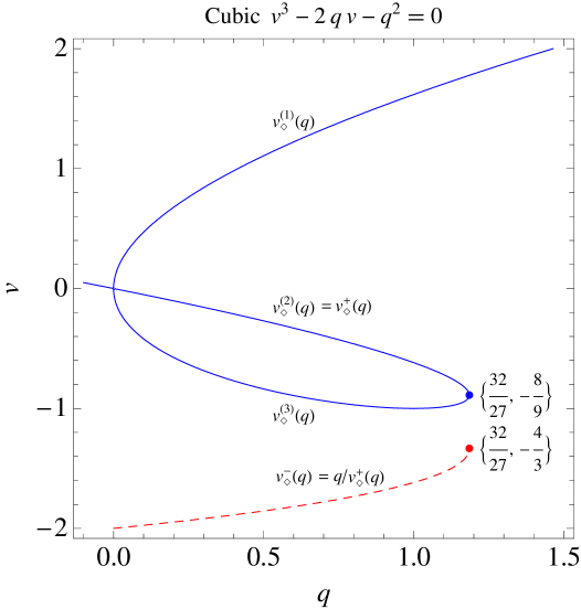
Figure 2: Solid blue curve shows the solutions of $v^{3}-2qv-q^{2}=0$. Dashed red curve shows the “dual” to the middle branch.

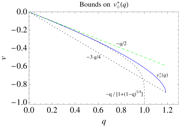
Figure 3: Solid blue curve shows $v_{\Diamond}^{+}(q)$. Dashed green line shows the upper bound $-q/2$. Dotted black curves show the lower bounds $-3q/4$ and (for $0\leq q\leq 1$) $-q/[1+(1-q)^{1/4}]$.

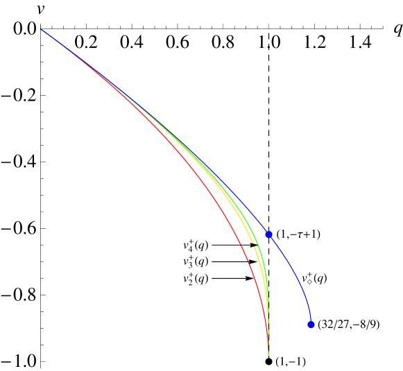
Figure 4: Solid blue curve shows $v_{\Diamond}^{+}(q)$. Solid red, yellow and green curves show $v_{m}^{+}(q)$ for $m=2,3,4$, respectively. Here $\tau=(1+\sqrt{5})/2$ is the golden ratio.

A central role in our analysis will be played by the fixed points of the diamond map, which satisfy $\Diamond_{q}(v)=v$ or equivalently (excluding the trivial fixed points $v=0$ and $v=+\infty$)

$$v^{3}-2qv-q^{2}\;=\;0\;.$$ (8.4)

The cubic (8.4) has one real root for $q<0$, three real roots for $0<q<32/27$, and one real root for $q>32/27$ (see Figure 2). For $0<q\leq 32/27$, let us denote by $v_{\Diamond}^{(i)}$ ($i=1,2,3$) the three roots of this cubic in decreasing order:

$$v_{\Diamond}^{(1)}\>>\;0\;>\;v_{\Diamond}^{(2)}\;\mathrel{\hbox to0.0pt{\lower 0.75pt\hbox{\kern-1.5pt\fourrm(\quad)}\hss}\raise 2.0pt\hbox{$\geq$}}\;v_{\Diamond}^{(3)}\;\mathrel{\hbox to0.0pt{\lower 0.75pt\hbox{\kern-1.5pt\fourrm(\quad)}\hss}\raise 2.0pt\hbox{$\geq$}}\;-1\;,$$ (8.5)

where the first (resp. second) inequality $\mathrel{\hbox to0.0pt{\lower 0.75pt\hbox{\kern-1.5pt\fourrm(\quad)}\hss}\raise 2.0pt\hbox{$\geq$}}$ is strict except at $q=32/27$ (resp. $q=1$). We are especially interested in the middle branch $v_{\Diamond}^{(2)}$, which we shall denote also by $v_{\Diamond}^{+}(q)$: it decreases monotonically from $v=0$ at $q=0$ to $v=-8/9$ at $q=32/27$, and is given explicitly by the horrendous expression

$$v_{\Diamond}^{+}(q) = \frac{3q}{2}\left[\{\textstyle{1\over 16}[27q-16+i\sqrt{27q(32-27q)}\,]\}^{1/3}\,e^{2\pi i/3}\;+\;\right.$$ (8.6)

$$\left.\quad\;+\;\{\textstyle{1\over 16}[27q-16+i\sqrt{27q(32-27q)}]\}^{-1/3}\,e^{-2\pi i/3}\;-\;1\right]^{-1}\qquad$$

or by the power series

$$v_{\Diamond}^{+}(q)\;=\;-\frac{q}{2}\,-\,\sum_{m=1}^{\infty}\frac{1}{2m\,8^{m}}{3m\choose m-1}\,q^{m+1}\;,$$ (8.7)

which is convergent for $|q|<32/27$ and shows that all derivatives of $v_{\Diamond}^{+}(q)$ are strictly negative for $0<q<32/27$. Putting $f(q,v)=v^{3}-2qv-q^{2}$, we have $f(q,-3q/4)\geq 0>f(q,-q/2)$ for all $0<q\leq 32/27$ and hence

$$-3q/4\;\leq\;v_{\Diamond}^{+}(q)\;<\;-q/2$$ (8.8)

[these bounds alternatively follow from the concavity of $v_{\Diamond}^{+}(q)$]. For $0<q<1$ we also have $f(q,-q/[1+(1-q)^{1/4}])>0$ and hence

$$v_{4}^{+}(q)\;\equiv\;-q/[1+(1-q)^{1/4}]\;<\;v_{\Diamond}^{+}(q)\;.$$ (8.9)

These bounds are illustrated in Figure 3. In Figure 4 we compare $v_{\Diamond}^{+}(q)$ with the functions $v_{2}^{+}(q)$, $v_{3}^{+}(q)$ and $v_{4}^{+}(q)$ introduced in the preceding section.

The fixed point $v_{\Diamond}^{+}(q)$ is repulsive for $0<q<32/27$ and becomes marginal at $q=32/27$: more precisely, the “multiplier”

$$\lambda_{\Diamond}(q)\;\equiv\;\left.{d\Diamond_{q}(v)\over dv}\right|_{v=v_{\Diamond}^{+}(q)}$$ (8.10)

decreases monotonically from $\lambda_{\Diamond}=+\infty$ at $q=0$ to $\lambda_{\Diamond}=+1$ at $q=32/27$.

We then define $v_{\Diamond}^{-}(q)$ to be the dual point

$$v_{\Diamond}^{-}(q)&\equiv{q\over v_{\Diamond}^{+}(q)}\\ =\frac{2}{3}\left[\{\textstyle{1\over 16}[27q-16+i\sqrt{27q(32-27q)}\,]\}^{1/3}\,e^{2\pi i/3}\;+\;\right.\\ \left.\quad+\;\{\textstyle{1\over 16}[27q-16+i\sqrt{27q(32-27q)}]\}^{-1/3}\,e^{-2\pi i/3}\;-\;1\right]\qquad\\ =-2\,+\,\sum_{m=1}^{\infty}\frac{2}{m\,8^{m}}{3m-2\choose m-1}\,q^{m}\;,$$ (8.11)

which increases monotonically, with all derivatives nonnegative, from $v=-2$ at $q=0$ to $v=-4/3$ at $q=32/27$ (see again Figure 2). Finally, we let $I_{\Diamond}(q)$ be the “diamond interval”

$$I_{\Diamond}(q)\;=\;\big{[}v_{\Diamond}^{-}(q),\,v_{\Diamond}^{+}(q)\big{]}\;.$$ (8.12)

The key facts about $v_{\Diamond}^{\pm}(q)$ are summarized in the following lemma, which will be proven at the end of this section:

Lemma 8.1

Let $0<q\leq 32/27$. Then:

• $v_{\Diamond}^{+}(q){\,\bowtie_{q}\,}v_{\Diamond}^{+}(q)=v_{\Diamond}^{-}(q)$.

• $v_{\Diamond}^{-}(q)\|v_{\Diamond}^{-}(q)=v_{\Diamond}^{+}(q)$.

• $I_{\Diamond}(q)$ is self-dual, i.e. it is invariant under $v\mapsto q/v$.

• $I_{\Diamond}(q)\|I_{\Diamond}(q)\subseteq I_{\Diamond}(q)$.

• $I_{\Diamond}(q){\,\bowtie_{q}\,}I_{\Diamond}(q)\subseteq I_{\Diamond}(q)$.

As a strong converse to Lemma 8.1(d,e), we have the following necessary condition for invariance under parallel and series connection:

Proposition 8.2

Let $q>0$ and let $\varnothing\neq{\mathcal{V}}\subset{\mathbb{R}}$ satisfy

• ${\mathcal{V}}\subseteq(-\infty,0)$

• If $v\in{\mathcal{V}}$, then $v\|v\in{\mathcal{V}}$.

• If $v\in{\mathcal{V}}$, then $v{\,\bowtie_{q}\,}v\in{\mathcal{V}}$.

Then $q\leq 32/27$ and ${\mathcal{V}}\subseteq I_{\Diamond}(q)$.

Please note that hypotheses (b) and (c) are weaker than ${\mathcal{V}}\|{\mathcal{V}}\subseteq{\mathcal{V}}$ and ${\mathcal{V}}{\,\bowtie_{q}\,}{\mathcal{V}}\subseteq{\mathcal{V}}$, as they require invariance only under “diagonal” parallel and series connection. Thus Proposition 8.2 immediately implies:

Corollary 8.3

Suppose that $q>0$ and ${\mathcal{V}}\neq\varnothing$ satisfies hypotheses (a)–(c) of Theorem 6.1. Then $q\leq 32/27$ and ${\mathcal{V}}\subseteq I_{\Diamond}(q)$.

In the special case of self-dual intervals ${\mathcal{V}}=(q/v_{+},v_{+})$ with $v_{+}<0$, we can give a necessary and sufficient condition to have invariance under parallel or series connection:

Proposition 8.4

Let $q>0$ and let ${\mathcal{V}}=(q/v_{+},v_{+})$ with $-\sqrt{q}<v_{+}<0$ (so that ${\mathcal{V}}\neq\varnothing$). Then the following are equivalent:

• ${\mathcal{V}}\|{\mathcal{V}}\subseteq{\mathcal{V}}$

• ${\mathcal{V}}{\,\bowtie_{q}\,}{\mathcal{V}}\subseteq{\mathcal{V}}$

• $q\leq 32/27$ and $\max[v_{\Diamond}^{(3)}(q),\,-q]\leq v_{+}\leq v_{\Diamond}^{(2)}(q)$.

Furthermore, we have

$$\max[v_{\Diamond}^{(3)}(q),\,-q]\;=\;\cases{-q&\hbox{\rm if } $0<q\leq 1$\cr\vskip 8.53581pt\cr v_{\Diamond}^{(3)}(q)&\hbox{\rm if } $1\leq q\leq 32/27$\cr}$$ (8.13)

The following further facts are relevant to the applicability of Theorem 6.1:

Lemma 8.5

• If $q>0$ and $v>0$, then $\Diamond_{q}^{k}(v)>0$ for all $k$.

• If $0<q\leq 32/27$ and $v_{\Diamond}^{+}(q)<v<0$, then $\Diamond_{q}(v)>v$, and $\Diamond_{q}^{k}(v)\geq 0$ for all sufficiently large $k$.

• If $q>32/27$ and $v<0$, then $\Diamond_{q}(v)>v$, and $\Diamond_{q}^{k}(v)\geq 0$ for all sufficiently large $k$.

• If $q\geq 1$ and $v\in{\mathbb{R}}$, then $\Diamond_{q}(v)\geq-q$, with strict inequality except when $(q,v)=(1,-1)$.

It follows that in cases (b) and (c), the sequence $\{\Diamond_{q}^{k}(v)\}_{k\geq 0}$ is strictly increasing as long as it stays negative; and once it goes nonnegative, it stays nonnegative (but need no longer be increasing). Note also that, in cases (b)–(d), if one iterate $\Diamond_{q}^{k}(v)$ ($k\geq 0$) happens to equal $-q/2$, then the next iterate and all subsequent iterates will equal $+\infty$ (which is indeed $\geq 0$).

Corollary 8.6

Let $G$ be a graph.

• If $0<q\leq 32/27$ and $v>v_{\Diamond}^{+}(q)$, then $Z_{\Diamond^{k}(G)}(q,v)>0$ for all sufficiently large $k$.

• If $0<q\leq 32/27$ and $v<v_{\Diamond}^{-}(q)$, then $Z_{\Diamond^{k}(G)^{(2)}}(q,v)>0$ for all sufficiently large $k$. [Here $G^{(2)}$ denotes the graph obtained from $G$ by replacing each edge by two parallel edges.]

• If $q>32/27$ and $v\in{\mathbb{R}}$, then $Z_{\Diamond^{k}(G)}(q,v)>0$ for all sufficiently large $k$.

We have already seen in Corollary 8.3 that if $q>0$ and ${\mathcal{V}}\neq\varnothing$ satisfy hypotheses (a)–(c) of Theorem 6.1, then $q\leq 32/27$ and ${\mathcal{V}}\subseteq I_{\Diamond}(q)$. We can now show, using Corollary 8.6, that if $m\geq 2$, $\gamma\in\{0,1\}$, $q>0$ and ${\mathcal{V}}\neq\varnothing$ satisfy the conclusion of Theorem 6.1 (with ${\mathcal{G}}\supseteq$ series-parallel graphs), then we must either have

• $\gamma=0$, $q<1$ and ${\mathcal{V}}\subseteq I_{\Diamond}(q)$

or else

• $\gamma=1$, $1<q\leq 32/27$ and ${\mathcal{V}}\subseteq I_{\Diamond}(q)$

— and this is so no matter how large we take $m$ to be.

Corollary 8.7

Fix $m\geq 2$, $\gamma\in\{0,1\}$ and $q>0$. Suppose that ${\mathcal{V}}\subset{\mathbb{R}}$ (${\mathcal{V}}\neq\varnothing$) satisfies the conclusion of Theorem 6.1 for some class ${\mathcal{G}}\supseteq$ series-parallel graphs. Then either:

• $\gamma=0$, $q<1$ and ${\mathcal{V}}\subseteq I_{\Diamond}(q)$; or

• $\gamma=1$, $1<q\leq 32/27$ and ${\mathcal{V}}\subseteq I_{\Diamond}(q)$.

Let us now prove all these results:

Proof of Lemma 8.1.  (a) The equation $v{\,\bowtie_{q}\,}v=q/v$ is precisely the cubic equation (8.4) satisfied by $v=v_{\Diamond}^{+}(q)$.

(b) follows from (a) by duality.

(c) is easy.

(d) Since $-2<v_{\Diamond}^{-}(q)<-1<v_{\Diamond}^{+}(q)<0$ by (8.8), the inequalities $-1<v_{\Diamond}^{+}(q)\|v_{\Diamond}^{+}(q)<v_{\Diamond}^{+}(q)$ and $v_{\Diamond}^{-}(q)<v_{\Diamond}^{+}(q)\|v_{\Diamond}^{-}(q)<-1$ are trivial. And by (b) we have the equality $v_{\Diamond}^{-}(q)\|v_{\Diamond}^{-}(q)=v_{\Diamond}^{+}(q)$.

(e) follows from (d) by duality.  $\Box$

Proof of Lemma 8.5.  (a) is obvious.

(b,c) If either $0<q\leq 32/27$ and $v_{\Diamond}^{+}(q)<v<0$, or $q>32/27$ and $v<0$, then the cubic (8.4) has the sign $v^{3}-2qv-q^{2}<0$. Since

$$\Diamond_{q}(v)-v\;=\;{v(v^{3}-2qv-q^{2})\over(q+2v)^{2}}\;,$$ (8.14)

it follows that $\Diamond_{q}(v)>v$ in these cases. (The value is unambiguously $+\infty$ if $v=-q/2$.)

Let us next prove that $\Diamond_{q}^{k}(v)\geq 0$ for all sufficiently large $k$. Note first that if $\Diamond_{q}^{k}(v)\geq 0$, then $\Diamond_{q}^{\ell}(v)\geq 0$ for all $\ell\geq k$, since $\Diamond_{q}$ obviously maps $[0,+\infty]$ into itself. So it suffices to prove that $\Diamond_{q}^{k}(v)\geq 0$ for at least one $k$. Assume the contrary: then, by virtue of what has already been shown, we have

$$v\,<\,\Diamond_{q}(v)\,<\,\Diamond_{q}^{2}(v)\,<\,\Diamond_{q}^{3}(v)\,<\,\ldots\,<\,0$$ (8.15)

and hence the sequence $\Diamond_{q}^{k}(v)$ tends to a limit $v_{*}$ satisfying $v<v_{*}\leq 0$ (and in particular $v_{*}>v_{\Diamond}^{+}(q)$ in case $q\leq 32/27$). Since $v_{*}$ must be a fixed point of $\Diamond_{q}$, the only possibility is $v_{*}=0$. But for $-q/2<v<0$ we have $\Diamond_{q}(v)>0$, which rules out the possibility that $\Diamond_{q}^{k}(v)$ tends to 0 from below.

(d) follows immediately from

$$\Diamond_{q}(v)+q\;=\;{(1+v)^{4}\,+\,(q-1)\Big{[}6\big{(}v+{q+1\over 3}\big{)}^{2}+{1\over 3}(q^{2}-q+1)\Big{]}\over(q+2v)^{2}}\;.$$ (8.16)

(The value is unambiguously $+\infty$ if $v=-q/2$.)  $\Box$

Proof of Corollary 8.6.  Since we are asserting that $Z_{G}>0$, it suffices to consider connected graphs $G$.

(a) We have $\Diamond_{q}^{k}(v)\geq 0$ for all sufficiently large $k$ by Lemma 8.5(a,b). So consider such a $k$. If none of the iterates $v,\Diamond_{q}(v),\Diamond_{q}^{2}(v),\ldots,\Diamond_{q}^{k-1}(v)$ happens to equal $-q/2$, then it follows from (8.2) that, for any graph $G$, the bivariate Tutte polynomial of the graph $\Diamond^{k}(G)$ satisfies

$$Z_{\Diamond^{k}(G)}(q,v)\;=\;\hbox{positive prefactors}\,\times\,Z_{G}(q,\Diamond_{q}^{k}(v))\;>\;0\;.$$ (8.17)

If, on the other hand, one of the iterates $\Diamond_{q}^{\ell}(v)$ [with $0\leq\ell\leq k-1$] equals $-q/2$, then it follows from (8.2) and (8.3) that

$$Z_{\Diamond^{k}(G)}(q,v)\;=\;\hbox{positive prefactors}\,\times\,q\,(q/2)^{4|E(\Diamond^{k-\ell-1}(G))|}\;>\;0\;.$$ (8.18)

(b) is an immediate consequence of (a), since $v<v_{\Diamond}^{-}(q)$ implies $v\|v>v_{\Diamond}^{+}(q)$.

(c) For all $q>32/27$ and $v\in{\mathbb{R}}$, we have $\Diamond_{q}^{k}(v)\geq 0$ for all sufficiently large $k$ by Lemma 8.5(a,c); so $Z_{\Diamond^{k}(G)}(q,v)>0$ by the same argument as in part (a).  $\Box$

Proof of Corollary 8.7.  We may show that either $\gamma=0$ and $q<1$ or else $\gamma=1$ and $q>1$ by an argument similar to that used in the proof of Proposition 6.3 (we leave the details to the reader). To show that $q\leq 32/27$ and ${\mathcal{V}}\subseteq I_{\Diamond}(q)$, suppose the contrary: then we use Corollary 8.6 with $G=K_{2}$ and $K_{3}$ to construct 2-connected series-parallel graphs $H$, with an arbitrarily large number of edges, whose vertex-set sizes have both parities. (Here we have used the fact that if $G$ is a non-separable graph, then $\Diamond^{k}(G)$ and $\Diamond^{k}(G)^{(2)}$ are both non-separable, and the parity of the size of their vertex sets is the same as that of $G$.) Since Corollary 8.6 yields $Z_{H}>0$ while the conclusion of Theorem 6.1 asserts that $(-1)^{|V(H)|-1+\gamma}Z_{H}>0$, one of the two parities yields a counterexample.  $\Box$

Proof of Proposition 8.2.  Hypotheses (a)–(c) imply in particular that $\Diamond_{q}({\mathcal{V}})\subseteq{\mathcal{V}}\subseteq(-\infty,0)$. By Lemma 8.5(a,b), this is possible with ${\mathcal{V}}\neq\varnothing$ only if $q\leq 32/27$ and ${\mathcal{V}}\subseteq(-\infty,v_{\Diamond}^{+}(q)]$. On the other hand, if $v<v_{\Diamond}^{-}(q)$, then [since $v_{\Diamond}^{-}(q)\leq-1$] we have $v\|v>v_{\Diamond}^{-}(q)\|v_{\Diamond}^{-}(q)=v_{\Diamond}^{+}(q)$. So, by hypothesis (b), we must have ${\mathcal{V}}\subseteq[v_{\Diamond}^{-}(q),v_{\Diamond}^{+}(q)]$.  $\Box$

Proof of Proposition 8.4.  Since ${\mathcal{V}}=(q/v_{+},v_{+})$ is self-dual, ${\mathcal{V}}\|{\mathcal{V}}\subseteq{\mathcal{V}}$ is equivalent to ${\mathcal{V}}{\,\bowtie_{q}\,}{\mathcal{V}}\subseteq{\mathcal{V}}$; so let us check the former. An obvious necessary condition is $q/v_{+}\leq-1\leq v_{+}$, i.e. $v_{+}\geq\max(-1,-q)$. If these conditions are satisfied, a necessary and sufficient condition is then

$$(q/v_{+})\|(q/v_{+})\;\leq\;v_{+}$$ (8.19)

or equivalently

$$v_{+}^{3}-2qv_{+}-q^{2}\;\geq\;0\;.$$ (8.20)

But this is just the “diamond cubic”, so we must have either $v_{+}\geq v_{\Diamond}^{(1)}(q)>0$ or else $v_{\Diamond}^{(2)}(q)\geq v_{+}\geq v_{\Diamond}^{(3)}(q)\geq-1$.

Finally, let us prove (8.13). We have $v^{3}-2qv-q^{2}\big{|}_{v=-q}=q^{2}-q^{3}$. For $0<q<1$ this is positive, so we must have $v_{\Diamond}^{(3)}(q)<-q<v_{\Diamond}^{(2)}(q)$. For $1<q\leq 32/27$ this is negative, so we must have either $-q<v_{\Diamond}^{(3)}(q)$ or $v_{\Diamond}^{(2)}(q)<-q<v_{\Diamond}^{(1)}(q)$; but the latter is excluded because we know that $-3q/4\leq v_{\Diamond}^{(2)}(q)$ by (8.8).  $\Box$

9 The interval $q\in(1,32/27]$

Let $G$ be a loopless graph with $n$ vertices, $c$ components, and $b$ nontrivial blocks; then Theorem 1.1(e) states that $P_{G}(q)$ is nonzero with sign $(-1)^{n+c+b}$ for $1<q\leq 32/27$ [15]. An analogous result also holds for loopless matroids [8]. In this section we shall use Theorem  6.1 to generalize these results to the multivariate Tutte polynomial. The multivariate approach allows us to replace the detailed graph-theoretic proof of [15] by a much simpler proof involving elementary calculus.

We need to find intervals ${\mathcal{V}}=(v_{-},v_{+})$ or ${\mathcal{V}}=[v_{-},v_{+}]$ satisfying hypotheses (a)–(d) of Theorem  6.1 with $\gamma=1$, for the case ${\mathcal{G}}=$ all graphs. For simplicity, let us restrict attention to self-dual intervals, i.e. $v_{-}=q/v_{+}$. Then invariance under parallel connection is equivalent to invariance under series connection; and by Proposition 8.4, these properties hold if and only if $q\leq 32/27$ and

$$\left\{\!\!\begin{array}[]{ll}-q&\hbox{if }0<q\leq 1\\[2.84526pt] v_{\Diamond}^{(3)}(q)&\hbox{if }1\leq q\leq 32/27\end{array}\!\!\right\}\;\leq\;v_{+}\;\leq\;v_{\Diamond}^{(2)}(q)\;.$$ (9.1)

Since $v_{\Diamond}^{(2)}(q)<-q/2$ by (8.8), hypothesis (a) is then satisfied as well. Finally, by Proposition 6.3, we can restrict attention to the case $q>1$.

It remains to determine the conditions under which also hypothesis (d) holds. We have been able to do this, and thus to find the optimal self-dual interval, for the cases $m=2$ and $m=3$.

Case $m=2$. The only non-separable graph with two edges is $K_{2}^{(2)}=C_{2}$. We want to have $Z_{K_{2}^{(2)}}(q,v_{1},v_{2})=q[q+(v_{1}\|v_{2})]>0$ for all $v_{1},v_{2}\in{\mathcal{V}}$, hence we need ${\mathcal{V}}\|{\mathcal{V}}\subseteq(-q,\infty)$ [actually it will be $\subseteq(-q,0)$]. Since $q>1$, the conditions $v_{+}\|v_{+}>-1>-q$ and $(q/v_{+})\|(q/v_{+})-1>-q$ hold trivially. So the only nontrivial condition is

$$v_{+}\|(q/v_{+})\;\geq\;-q$$ (9.2)

or equivalently

$$v_{+}^{2}+2qv_{+}+q\;\leq\;0\;.$$ (9.3)

This means that $v_{+}$ must lie between the two roots of the quadratic (9.3), which are $-q\pm\sqrt{q^{2}-q}$. Of course, we must also make sure that $v_{\Diamond}^{(3)}(q)\leq v_{+}\leq v_{\Diamond}^{(2)}(q)$ to satisfy hypotheses (a)–(c). The maximal choice $v_{+}=-q+\sqrt{q^{2}-q}$ works whenever $1<q\leq 9/8$. Otherwise the best we can do is to take $v_{+}=v_{\Diamond}^{(2)}(q)\equiv v_{\Diamond}^{+}(q)$. We have therefore proven:

Corollary 9.1

Let $1<q\leq 32/27$ and define

$${\mathcal{V}}_{2}\;=\;\cases{\big{(}-q-\sqrt{q^{2}-q},\>-q+\sqrt{q^{2}-q}\,\big{)}&if $1<q\leq 9/8$\cr\vskip 8.53581pt\cr I_{\Diamond}(q)\,\equiv\,[v_{\Diamond}^{-}(q),v_{\Diamond}^{+}(q)]&if $9/8\leq q\leq 32/27$\cr}$$ (9.4)

Then $(-1)^{n+c+b}Z_{G}({q,{\bf v}})>0$ whenever $G=(V,E)$ is a loopless bridgeless graph with $n$ vertices, $c$ components and $b$ nontrivial blocks, and $v_{e}\in{\mathcal{V}}_{2}$ for all $e\in E$.

The interval ${\mathcal{V}}_{2}$ is the best possible self-dual interval for Corollary 9.1, in the following senses:

(i) For all $q>1$, the graph $K_{2}^{(2)}$ has a multivariate root at $v_{1}=-q-\sqrt{q^{2}-q}$, $v_{2}=-q+\sqrt{q^{2}-q}$.

(ii) For $1<q\leq 32/27$, $v>v_{\Diamond}^{+}(q)$, and $G$ an arbitrary graph, the graph $\Diamond^{k}(G)$ satisfies $Z_{\Diamond^{k}(G)}(q,v)>0$ by Corollary 8.6(a). This has the wrong sign for Corollary 9.1 when $G$ is 2-connected with an odd number of vertices. A similar argument holds if $1<q\leq 32/27$ and $v<v_{\Diamond}^{-}(q)$, or $q>32/27$ and $v\in{\mathbb{R}}$, using Corollary 8.6(b) and (c), respectively.

Case $m=3$. The only non-separable graphs with two edges are $K_{2}^{(3)}$ and its dual $C_{3}$. By self-duality, it suffices to consider the former. We want to have $Z_{K_{2}^{(3)}}(q,v_{1},v_{2},v_{3})=q[q+(v_{1}\|v_{2}\|v_{3})]>0$ for all $v_{1},v_{2},v_{3}\in{\mathcal{V}}$, hence we need ${\mathcal{V}}\|{\mathcal{V}}\|{\mathcal{V}}\subseteq(-q,\infty)$ [again it will actually be $\subseteq(-q,0)$]. Since $q>1$, it is easy to see that $|1+q/v_{+}|>|1+v_{+}|$, i.e. the interval ${\mathcal{V}}$ extends farther to the left of $-1$ than to the right. Therefore, the necessary and sufficient condition to have ${\mathcal{V}}\|{\mathcal{V}}\|{\mathcal{V}}\subseteq(-q,\infty)$ is simply

$$(q/v_{+})\|(q/v_{+})\|(q/v_{+})\;\geq\;-q$$ (9.5)

or equivalently

$$v_{+}^{3}+3v_{+}^{2}+3qv_{+}+q^{2}\;\leq\;0\;.$$ (9.6)

For $q>1$ this cubic has a single real root $v_{+}=-1+(q-1)^{1/3}-(q-1)^{2/3}$, so the inequality (9.6) reduces to

$$v_{+}\;\leq\;-1\,+\,(q-1)^{1/3}\,-\,(q-1)^{2/3}\;.$$ (9.7)

Of course, we must also make sure that $v_{\Diamond}^{(3)}(q)\leq v_{+}\leq v_{\Diamond}^{(2)}(q)$ in order to satisfy hypotheses (a)–(c). The maximal choice $v_{+}=-1+(q-1)^{1/3}-(q-1)^{2/3}$ works whenever $1<q\leq 9/8$. (It is an amazing coincidence — for which we have no deep explanation — that both $m=2$ and $m=3$ give rise to the same crossover point $q=9/8$.) Otherwise the best we can do is to take $v_{+}=v_{\Diamond}^{(2)}(q)\equiv v_{\Diamond}^{+}(q)$. We have therefore proven:

Corollary 9.2

Let $1<q\leq 32/27$ and define

$${\mathcal{V}}_{3}\;=\;\cases{\biggl{(}\,\displaystyle{q\over-1+(q-1)^{1/3}-(q-1)^{2/3}},\,-1+(q-1)^{1/3}-(q-1)^{2/3}\biggr{)}&if $1<q\leq 9/8$\cr\vskip 5.69054pt\cr I_{\Diamond}(q)\,\equiv\,[v_{\Diamond}^{-}(q),v_{\Diamond}^{+}(q)]&if $9/8\leq q\leq 32/27$\cr\vskip 1.0pt\cr}$$ (9.8)

Then $(-1)^{n+c+b}Z_{G}({q,{\bf v}})>0$ whenever $G=(V,E)$ is a graph with $n$ vertices, $c$ components and $b$ blocks, in which each block contains at least three edges, and $v_{e}\in{\mathcal{V}}_{3}$ for all $e\in E$.

We can show that the interval ${\mathcal{V}}_{3}$ is best possible in the same way as for the interval ${\mathcal{V}}_{2}$ of Corollary 9.1. Suppose $1<q\leq 9/8$. If either $v_{1}=v_{2}=v_{3}<q/[-1+(q-1)^{1/3}-(q-1)^{2/3}]$ and $G=K_{2}^{(3)}$, or $v_{1}=v_{2}=v_{3}<q/[-1+(q-1)^{1/3}-(q-1)^{2/3}]$, and $G=C_{3}$, then $Z_{G}(q,{q,{\bf v}})$ has the wrong sign. So the interval ${\mathcal{V}}_{3}$ is best possible for $1<q\leq 9/8$, even in the univariate case, and even allowing subsets ${\mathcal{V}}$ that are not necessarily intervals and not necessarily self-dual. When $q>9/8$, the argument is the same as that given for ${\mathcal{V}}_{2}$.

We close this section by extending our results to matroids. Since all matroids with at most three elements are graphic, Corollaries 9.1 and 9.2 and Theorem 6.4 immediately imply:

Corollary 9.3

Let $1<q\leq 32/27$ and $m\in\{2,3\}$, and let ${\cal V}_{2}$ and ${\cal V}_{3}$ be the intervals defined in Corollaries 9.1 and 9.2, respectively. Then $(-1)^{r(M)+b}\widetilde{Z}_{M}({q,{\bf v}})>0$ whenever $M$ is a matroid of rank $r(M)$ on the ground set $E$ that has $b$ $2$-connected components, in which each $2$-connected component contains at least $m$ elements, and $v_{e}\in{\mathcal{V}}_{m}$ for all $e\in E$.

10 Further refinements?

Let us conclude by making some remarks on the possibility of extending the zero-free regions obtained in Sections 7 and 9 to larger values of $m$. We conjecture that for $0<q<1$ and $1<q\leq 32/27$, there exists a strictly increasing family of self-dual intervals ${\mathcal{V}}_{m}(q)=(q/v_{m}^{+}(q),v_{m}^{+}(q))$ that satisfy the hypotheses of Theorem 6.1 for the case ${\mathcal{G}}=$ all graphs, and such that $\lim\limits_{m\to\infty}{\mathcal{V}}_{m}(q)=I_{\Diamond}(q)$. If true, this would imply:

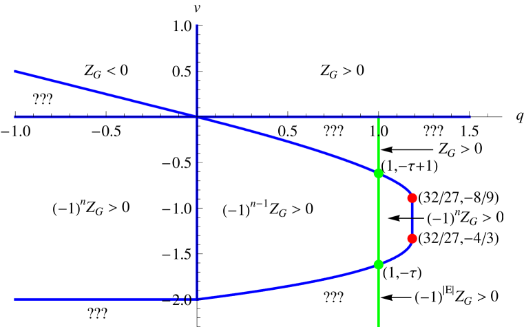
Figure 5: Conjectured limiting regions as $m\to\infty$ in which the sign of $Z_{G}(q,{\bf v})$ can be controlled for loopless 2-connected graphs $G$ with at least $m$ edges. Here $\tau=(1+\sqrt{5})/2$ is the golden ratio.

Conjecture 10.1

Suppose $0<q<1$. Then there exists a strictly increasing sequence of self-dual intervals ${\mathcal{V}}_{m}(q)$, $m\geq 2$, such that

• $\lim\limits_{m\to\infty}{\mathcal{V}}_{m}(q)=I_{\Diamond}(q)$, and

• $(-1)^{n-1}Z_{G}(q,{\bf v})>0$ for all for all $2$-connected graphs $G=(V,E)$ with $n$ vertices, at least $m$ edges, and $v_{e}\in{\mathcal{V}}_{m}(q)$ for all $e\in E$.

Conjecture 10.2

Suppose $1<q\leq 32/27$. Then there exists a strictly increasing sequence of self-dual intervals ${\mathcal{V}}_{m}(q)$, $m\geq 2$, such that

• $\lim\limits_{m\to\infty}{\mathcal{V}}_{m}(q)=I_{\Diamond}(q)$, and

• $(-1)^{n}Z_{G}(q,{\bf v})>0$ for all for all $2$-connected graphs $G=(V,E)$ with $n$ vertices, at least $m$ edges, and $v_{e}\in{\mathcal{V}}_{m}(q)$ for all $e\in E$.

These conjectures are illustrated in Figure 5.

For any fixed $m$, intervals ${\mathcal{V}}_{m}(q)$ satisfying the hypotheses of Theorem 6.1 can in principle be found by a finite amount of calculation (i.e., there are finitely many $m$-edge 2-connected graphs to consider), but the computations seem rather messy for $m\geq 5$. For instance, for $m=5$ we have not only the 5-cocycle and the 5-cycle, but also the triangle with two double edges, its dual $K_{4}\setminus e$, the triangle with one triple edge, and its dual $C_{4}$ with one double edge. Indeed, for $m\geq 5$ the interval $I_{m}$ defined in (7.9), which arises by considering only the $m$-cocycle and the $m$-cycle, cannot satisfy the hypotheses of Theorem 6.1 for small $q>0$, as it fails to be contained in $I_{\Diamond}(q)$:

$$v_{\Diamond}^{+}(q) = -{q\over 2}\,-\,{q^{2}\over 16}\,-\,O(q^{3})$$ (10.1)

$$-\,{q\over 1+(1-q)^{1/m}} = -{q\over 2}\,-\,{q^{2}\over 4m}\,-\,O(q^{3})$$ (10.2)

The behaviors expected for $0<q<1$ and for $1<q\leq 32/27$ also differ in a curious way. For $0<q<1$ we expect that the upper endpoints $v_{m}^{+}(q)$ of the intervals ${\mathcal{V}}_{m}(q)$ will be strictly increasing towards $v_{\Diamond}^{+}(q)$. For $1<q\leq 32/27$, by contrast, we already have $v_{m}^{+}(q)=v_{\Diamond}^{+}(q)$ exactly for $m=2,3$ when $9/8\leq q\leq 32/27$; for larger $m$ we can expect this “crossover point” $q=9/8$ to move downwards towards $q=1$. That, at any rate, is our naive guess based on the behavior for small $m$.

Let us note that Conjectures 10.1 and 10.2 are in a certain sense the most one can hope for, because we have shown in Corollary 8.7 that conclusion (b) of Conjecture 10.1 can only hold if $q<1$ and ${\mathcal{V}}_{m}(q)\subseteq I_{\Diamond}(q)$, and that conclusion (b) of Conjecture 10.2 can only hold if $1<q\leq 32/27$ and ${\mathcal{V}}_{m}(q)\subseteq I_{\Diamond}(q)$.

But we can pose the question more broadly, by asking about the regions (beyond those covered by Conjectures 10.1 and 10.2) where we have not succeeded in controlling the sign of $Z_{G}(q,{\bf v})$, namely:

• $q<0$ and $v<-2$;

• $q<0$ and $0<v<-q/2$;

• $0<q\leq 32/27$ ($q\neq 1$) and $v<v_{\Diamond}^{-}(q)$;

• $0<q\leq 32/27$ ($q\neq 1$) and $v_{\Diamond}^{+}(q)<v<0$;

• $q>32/27$ and $v<0$.

(These regions are labelled ??? in Figure 5.) We conjecture that if ${\mathcal{V}}$ contains any points in these regions, then there is no hope of controlling the sign of $Z_{G}(q,{\bf v})$, at least in terms of the numbers of vertices and edges, because both signs are possible, even for the bivariate Tutte polynomial $Z_{G}(q,v)$:

Conjecture 10.3

Fix $q$ and $v$ real, and suppose that we are in one of the cases (a)–(e) above. Then, for all sufficiently large $n$ (how large depends on $q$ and $v$) and all sufficiently large $m$ (how large depends on $q$, $v$ and $n$), there exist 2-connected graphs $G$ with $n$ vertices and $m$ edges that make $Z_{G}(q,v)$ nonzero with either sign.

We furthermore suspect that for $0<q\leq 32/27$ (and perhaps all the way up to $q=2$) the graphs in Conjecture 10.3 can be taken to be series-parallel. On the other hand, one cannot use series-parallel graphs when $q>2$ and $v\geq-1$, for it is known that $Z_{G}(q,{\bf v})>0$ in this region [30, Proposition 6.3 and Corollary 6.4]. More generally, it is known that for graphs of tree-width $\leq k$, we have $Z_{G}(q,{\bf v})>0$ whenever $q>k$ and $v\geq-1$ [32, Theorem 3.4].

If Conjecture 10.3 is correct, it follows that the results in this paper, together with Conjectures 10.1 and 10.2, are in a fairly strong sense best possible.

We actually conjecture that our results in this paper, together with Conjectures 10.1 and 10.2, are best possible in a much stronger sense than that given by Conjecture 10.3, namely:

Conjecture 10.4

The zeros of the bivariate Tutte polynomials $Z_{G}(q,v)$ are dense in regions (a)–(e) as $G$ ranges over all graphs. Here “dense” means either that the zeros are dense in $v$ for each fixed $q$, or dense in $q$ for each fixed $v$.

It is possible that Conjectures 10.3 and 10.4 can be proven, at least in cases (c), (d) and (e), by a variant of the constructions used by Thomassen [32, Proposition 2.3 and Theorem 2.5].

References

- [1] G.D. Birkhoff, A determinantal formula for the number of ways of coloring a map, Ann. Math. 14 (1912), 42–46.
- [2] J.I. Brown and C.A. Hickman, On chromatic roots of large subdivisions of graphs, Discrete Math. 242 (2002), 17–30.
- [3] T. Brylawski and J. Oxley, The Tutte polynomial and its applications, in N. White (editor), Matroid Applications, Encyclopedia of Mathematics and its Applications #40 (Cambridge University Press, Cambridge, 1992), pp. 123–225.
- [4] G. Chartrand, A. Kaugars and D.R. Lick, Critically -connected graphs, Proc. Amer. Math. Soc. 32 (1972), 63–68.
- [5] G.L. Chia, A bibliography on chromatic polynomials, Discrete Math. 172 (1997), 175–191.
- [6] B. Derrida, L. De Seze and C. Itzykson, Fractal structure of zeros in hierarchical models, J. Stat. Phys. 33 (1983), 559–569.
- [7] F.-M. Dong, private communication (June 2008).
- [8] H. Edwards, R. Hierons and B. Jackson, The zero-free intervals for characteristic polynomials of matroids, Combin. Probab. Comput. 7 (1998), 153–165.
- [9] R.G. Edwards and A.D. Sokal, Generalization of the Fortuin-Kasteleyn-Swendsen-Wang representation and Monte Carlo algorithm, Phys. Rev. D 38 (1988), 2009–2012.
- [10] Y. Egawa, Contractible edges in -connected graphs with minimum degree greater than or equal to , Graphs Combin. 7 (1991), 15–21.
- [11] C.M. Fortuin and P.W. Kasteleyn, On the random-cluster model. I. Introduction and relation to other models, Physica 57 (1972), 536–564.
- [12] D.D. Gebhard and B.E. Sagan, Sinks in acyclic orientations of graphs, J. Combin. Theory B 80 (2000), 130–146.
- [13] C. Greene and T. Zaslavsky, On the interpretation of Whitney numbers through arrangements of hyperplanes, zonotopes, non-Radon partitions, and orientations of graphs, Trans. Amer. Math. Soc. 280 (1983), 97–126.
- [14] C. Itzykson and J.M. Luck, Zeroes of the partition function for statistical models on regular and hierarchical lattices, in V. Ceauşescu, G. Costache and V. Georgescu (editors), Critical Phenomena (1983 Brasov School Conference) (Birkhäuser, Boston–Basel–Stuttgart, 1985), pp. 45–82.
- [15] B. Jackson, A zero-free interval for chromatic polynomials of graphs, Combin. Probab. Comput. 2 (1993), 325–336.
- [16] B. Jackson, Zeros of chromatic and flow polynomials of graphs, J. Geom. 76 (2003), 95–109, math.CO/0205047 at arXiv.org.
- [17] P.W. Kasteleyn and C.M. Fortuin, Phase transitions in lattice systems with random local properties, J. Phys. Soc. Japan 26 (Suppl.) (1969), 11–14.
- [18] M. Kriesell, A degree sum condition for the existence of a contractible edge in a -connected graph, J. Combin. Theory B 82 (2001), 81–101.
- [19] J.G. Oxley, On minor-minimally-connected matroids, Discrete Math. 51 (1984), 63–72.
- [20] J.G. Oxley, Matroid Theory (Oxford University Press, New York, 1992).
- [21] J.G. Oxley, On the interplay between graphs and matroids, in Surveys in Combinatorics, 2001, edited by J.W.P. Hirschfeld (Cambridge University Press, Cambridge, 2001), pp. 199–239.
- [22] R.B. Potts, Some generalized order-disorder transformations, Proc. Cambridge Philos. Soc. 48 (1952), 106–109.
- [23] R.C. Read, An introduction to chromatic polynomials, J. Combin. Theory 4 (1968), 52–71.
- [24] R.C. Read and W.T. Tutte, Chromatic polynomials, in L.W. Beineke and R.J. Wilson (editors), Selected Topics in Graph Theory 3 (Academic Press, London, 1988), pp. 15–42.
- [25] G. Royle and A.D. Sokal, The Brown–Colbourn conjecture on zeros of reliability polynomials is false, J. Combin. Theory B 91 (2004), 345–360, math.CO/0301199 at arXiv.org.
- [26] J. Salas and A.D. Sokal, Transfer matrices and partition-function zeros for antiferromagnetic Potts models. I. General theory and square-lattice chromatic polynomial, J. Stat. Phys. 104 (2001), 609–699, cond-mat/0004330 at arXiv.org.
- [27] A.D. Scott and A.D. Sokal, The repulsive lattice gas, the independent-set polynomial, and the Lovász local lemma, J. Statist. Phys. 118 (2005), 1151–1261, cond-mat/0309352 at arXiv.org.
- [28] R. Shrock, Chromatic polynomials and their zeros and asymptotic limits for families of graphs, Discrete Math. 231 (2001), 421–446, cond-mat/9908387 at arXiv.org.
- [29] A.D. Sokal, Bounds on the complex zeros of (di)chromatic polynomials and Potts-model partition functions, Combin. Probab. Comput. 10 (2001), 41–77, cond-mat/9904146 at arXiv.org.
- [30] A.D. Sokal, Chromatic roots are dense in the whole complex plane, Combin. Probab. Comput. 13 (2004), 221–261, cond-mat/0012369 at arXiv.org.
- [31] A.D. Sokal, The multivariate Tutte polynomial (alias Potts model) for graphs and matroids, in Surveys in Combinatorics, 2005, edited by Bridget S. Webb (Cambridge University Press, Cambridge–New York, 2005), pp. 173–226, math.CO/0503607 at arXiv.org.
- [32] C. Thomassen, The zero-free intervals for chromatic polynomials of graphs, Combin. Probab. Comput. 6 (1997), 497–506.
- [33] W.T. Tutte, A ring in graph theory, Proc. Cambridge Philos. Soc. 43 (1947), 26–40.
- [34] W.T. Tutte, A contribution to the theory of chromatic polynomials, Canad. J. Math. 6 (1954), 80–91.
- [35] D.G. Wagner, Zeros of reliability polynomials and -vectors of matroids, Combin. Probab. Comput. 9 (2000), 167–190.
- [36] H. Whitney, A logical expansion in mathematics, Bull. Amer. Math. Soc. 38 (1932), 572–579.
- [37] F.Y. Wu, The Potts model, Rev. Mod. Phys. 54 (1982), 235–268; erratum 55 (1983), 315.
- [38] F.Y. Wu, Potts model of magnetism (invited), J. Appl. Phys. 55 (1984), 2421–2425.