UAB-FT–647

June 2008

Top Quark Compositeness: Feasibility and Implications

Alex Pomarol and Javi Serra

IFAE, Universitat Autònoma de Barcelona, 08193 Bellaterra, Barcelona

In models of electroweak symmetry breaking in which the SM fermions get their masses by mixing with composite states, it is natural to expect the top quark to show properties of compositeness. We study the phenomenological viability of having a mostly composite top. The strongest constraints are shown to mainly come from one-loop contributions to the $T$-parameter. Nevertheless, the presence of light custodial partners weakens these bounds, allowing in certain cases for a high degree of top compositeness. We find regions in the parameter space in which the $T$-parameter receives moderate positive contributions, favoring the electroweak fit of this type of models. We also study the implications of having a composite top at the LHC, focusing on the process $pp\rightarrow t\bar{t}t\bar{t}(b\bar{b})$ whose cross-section is enhanced at high-energies.

1 Introduction

Unraveling the origin of the electroweak symmetry breaking (EWSB) is the main priority of the LHC. One possibility, inspired by QCD, is that EWSB occurs in a new strong sector at energies of few TeV. Examples of this realization are Technicolor models [1] and composite Higgs scenarios [2]. More recently, due to the connection between strongly-coupled theories and gravity on warped extra dimensions, these scenarios have been studied in the framework of five-dimensional theories (see for example, Refs. [3, 4]).

In all these examples the SM fields that get masses from EWSB must at least be coupled to this new (strong) sector with a strength proportional to their masses. This suggests that the top quark is the SM field with the largest coupling to the new sector, and therefore the most sensitive to new physics. If this is the case, the top is the most likely SM fermion to show signals of compositeness. Knowing the degree of compositeness of the top is then very important to understand the physics lying beyond the SM.

The aim of this paper is twofold. First, we want to study the viability of having a top quark being mostly a composite state. We will study this possibility in a framework, inspired by extra-dimensional models, in which the SM fermions are a mixture of elementary and composite states, with a mixing angle proportional to $\sqrt{m_{f}}$, where $m_{f}$ is the fermion mass. We will take the limit in which one of the two chiral components of the top is mostly a composite state, and study the phenomenological viability of this limit. The main constraints from present experiments will arise from the $T$-parameter. We will calculate the one-loop contributions to $T$ and show under which conditions a composite top is allowed. An important role will be played by the custodial partners of the top, the custodians, that become light in the composite limit and reduce significantly the total contribution to $T$. Our results will also be useful to determine how a positive contribution to $T$ can arise, as required, in this class of models, to accommodate a large and positive $S$-parameter.

Secondly, we will show how future experiments can test the properties of the top and tell us about the degree of its compositeness. We will do this by following a model-independent approach, similar to Ref. [5], in which the top compositeness is characterized by few higher-dimensional operators. We will concentrate on the study of the process $pp\rightarrow t\bar{t}t\bar{t}(b\bar{b})$ that, for a composite top, is enhanced at high-energies. We will calculate the cross-section of this process and show how different observables can be used to distinguish between a composite and elementary top.

The organization of the paper is as follows. In section 2 we present a framework for a composite top. Its low-energy effective lagrangian is given in section 3. The experimental constraints are presented in section 4; we study the effects on $Zb\bar{b}$ and the one-loop contributions to the $T$-parameter. We present the regions of the parameter space in which a composite top is allowed. In section 5 we show how to study the top properties at future experiments and present the calculation for $pp\rightarrow t\bar{t}t\bar{t}(b\bar{b})$. We conclude in section 6.

2 Framework

The framework we want to consider is the following. We will assume that beyond the SM there is a new sector (the BSM sector), characterized by two parameters, a generic coupling $g_{\rho}$ and a mass scale $M_{\rho}$. We will be mostly interested in the limit $1<g_{\rho}\lesssim 4\pi$ such that the BSM sector consists of resonances whose coupling, although large, allows us for a perturbative expansion. Our analysis, however, will be able to be extended to the region $g_{\rho}\sim 4\pi$ corresponding to a maximally strongly-coupled BSM. The scale $M_{\rho}$, in analogy with QCD, will correspond to the mass of the lightest resonance. Examples of this class of models are strongly-coupled gauge theories in the large-$N$ limit or extra dimensional models [3, 4].

We will also assume that this new sector is responsible for the EWSB. This means that the Goldstone bosons $G^{a}$ (to be eaten by the $W$ and $Z$) will arise from the BSM sector. They can be parametrized by a matrix $\Sigma$ whose vacuum expectation value (VEV) breaks the EW symmetry:

$$\Sigma=v\,e^{i\sigma^{a}G^{a}/v}\ ,\ \ {\rm where}\ \ v\simeq 246\ {\rm GeV}\,.$$ (1)

In Higgsless theories $v$ is equal to the decay constants of the Goldstones $f$ which can be written as

$$f=\frac{M_{\rho}}{g_{\rho}}\,.$$ (2)

In theories in which the Higgs arises from the BSM sector as a Pseudo-Goldstone Boson (PGB) the scale $f$, satisfying Eq. (2), is associated to the PGB-Higgs decay constant. The EW scale $v$ is determined in these models by minimizing the Higgs potential and one generically obtains $v\lesssim f$ [2, 4]. To incorporate both scenarios, Higgsless and composite Higgs, we will parametrize the deviation of $v$ from $f$ by the dimensionless parameter $\xi$ defined by [5]

$$\xi=\frac{v^{2}}{f^{2}}\leq 1\,.$$ (3)

Electroweak precision tests (EWPT) put tight constraints on models of this class, since the BSM resonances induce sizable tree-level modifications of the SM gauge propagators. The main effects can be parametrized by two quantities, the $S$ and $T$ parameters [6]. The tree-level contribution to $T$ can vanish if the BSM sector is invariant under a global SU(2)_V symmetry, the so-called custodial symmetry. For this reason, we will assume that the BSM sector is invariant under a global SU(2)${}_{L}\times$SU(2)_R under which the Goldstone multiplet $\Sigma$ transforms as a ${\bf(2,2)}$. The VEV of $\Sigma$ will break SU(2)${}_{L}\times$SU(2)_R down to the diagonal subgroup corresponding to the custodial symmetry. We will further impose that the BSM sector is also invariant under the discrete symmetry $P_{LR}$ that interchanges $L\leftrightarrow R$. As we will see later, this extra parity is crucial to avoid large corrections to $Zb\bar{b}$ [7]. Under these assumptions the only important tree-level constraint on this class of models comes from the $S$-parameter. In extra dimensional models in which $S$ is calculable one finds, barring cancellations, the bound $M_{\rho}\gtrsim 2.3$ TeV [4], or equivalently,

$$f\gtrsim 500\ {\rm GeV}\ \ \ (\xi\lesssim 1/4)\ \ \ {\rm for}\ \ g_{\rho}\sim 4.6\,.$$ (4)

We could reduce the lower bound on $f$ to reach the Higgsless limit $\xi=1$, but at the prize of having a very large $g_{\rho}$. In this case the value of $S$ can only be estimated, since it cannot be calculated by any perturbative method. In deriving Eq. (4) we have assumed that $T$ receives a large and positive contribution, $\alpha\Delta T\sim 1-4\cdot 10^{-3}$, beyond that of the SM. As we will see later, this can arise from one-loop effects that can be sizable if the top is composite.

Finally, in the fermionic sector we will take the following extra assumption. The SM fermions will be assumed to be linearly coupled to the BSM resonances. This means that exists a basis in which the SM fermions couple to the BSM sector only through mass mixing terms. In particular, for the top we have

$$\mathcal{L}=y_{L}f\,\bar{q}_{L}^{\rm el}\mathcal{P}_{q}[Q_{R}]+y_{R}f\,\bar{t}_{R}^{\rm el}\mathcal{P}_{t}[T_{L}]+M_{Q}\bar{Q}_{L}Q_{R}+M_{T}\bar{T}_{R}T_{L}+g_{\rho}\bar{Q}_{L}\Sigma T_{R}+\cdots\,,$$ (5)

where ${q}_{L}^{\rm el}$ and ${t}_{R}^{\rm el}$ denote the elementary left-handed top-bottom doublet and right-handed top respectively, and $Q_{L,R}$ and $T_{L,R}$ are vector-like “composite” BSM resonances. The operators $\mathcal{P}_{q}$ and $\mathcal{P}_{t}$ project the BSM resonances into components with the SM quantum numbers of $q_{L}^{\rm el}$ and $t_{R}^{\rm el}$ respectively. We will consider that there is only one $Q_{L,R}$ and $T_{L,R}$ resonance. In five-dimensional theories this corresponds to keep only the lightest Kaluza-Klein (KK) state of each tower that it is usually a good approximation [8]. Apart from the mass terms, we have included in Eq. (5) the Yukawa term $\bar{Q}_{L}\Sigma T_{R}$ responsible, as we will see, for the top mass. The absence in Eq. (5) of bilinear couplings of elementary fields with the BSM resonances, e.g. $\bar{q}^{\rm el}_{L}\Sigma t^{\rm el}_{R}$, is a feature of holographic models [4]. It was also implemented in Technicolor models in Ref. [9]. This implies that the top get a mass through mixing with BSM states. This way of generating fermion masses is phenomenologically favorable, since it avoids dangerous flavor transitions [4] that were present in the original Technicolor models. For our analysis here, however, the presence of terms like $\bar{q}^{\rm el}_{L}\Sigma t^{\rm el}_{R}$ would only introduce more parameters but would not qualitatively change our conclusions.

The SM top components, $q_{L}$ and $t_{R}$, are identified with the massless states (before EWSB). These are given by

$$q_{L} = \cos{\theta_{L}}\,q_{L}^{\rm el}+\sin{\theta_{L}}\,\mathcal{P}_{q}[Q_{L}]\ ,\quad\tan{\theta_{L}}=\frac{y_{L}f}{M_{Q}}\,,$$

$$t_{R} = \cos{\theta_{R}}\,t_{R}^{\rm el}+\sin{\theta_{R}}\,\mathcal{P}_{t}[T_{R}]\ ,\quad\tan{\theta_{R}}=\frac{y_{R}f}{M_{T}}\,.$$ (6)

The orthogonal states get a mass squared $M^{2}_{Q}+y^{2}_{L}f^{2}$ and $M^{2}_{T}+y^{2}_{R}f^{2}$. The last term of Eq. (5) gives, after the above rotation, the Yukawa coupling of the top:

$$y_{t}=g_{\rho}\sin{\theta_{L}}\sin{\theta_{R}}\,.$$ (7)

By requiring a top mass $m_{t}=y_{t}v\simeq 160$ GeV (at energies $M_{\rho}\sim 1$ TeV), Eq. (7) gives a lower bound for the mixing angles, $\sin\theta_{L,R}\gtrsim 0.6/g_{\rho}$. The largeness of these mixing angles makes natural the possibility that one of the two chiralities of the top is fully composite. We will consider this possibility below.

2.1 The top composite limit

We are interested in exploring the limit in which either $q_{L}^{\rm el}$ or $t_{R}^{\rm el}$ is maximally coupled to the BSM sector such that the SM $q_{L}$ or $t_{R}$ mostly corresponds to a composite BSM state. For the left-handed top, this corresponds to the limit

$$\left\{\begin{array}[]{c}\sin{\theta_{L}}\rightarrow 1\\ y_{L}\rightarrow g_{\rho}\end{array}\right\}\quad\textnormal{and}\quad\left\{\begin{array}[]{c}\sin{\theta_{R}}\rightarrow y_{t}/g_{\rho}\\ y_{R}\simeq y_{t}\end{array}\right\}\,.$$ (8)

For the right-handed top, the composite limit is given by

$$\left\{\begin{array}[]{c}\sin{\theta_{R}}\rightarrow 1\\ y_{R}\rightarrow g_{\rho}\end{array}\right\}\quad\textnormal{and}\quad\left\{\begin{array}[]{c}\sin{\theta_{L}}\rightarrow y_{t}/g_{\rho}\\ y_{L}\simeq y_{t}\end{array}\right\}\,.$$ (9)

In warped extra-dimensional models these limits can be obtained by taking negative values for the 5D mass of the left-handed (or right-handed) top that localizes the 4D massless state towards the IR-boundary [4]. Although the composite limit can also be considered for other SM fermions, the fact that the top is the heaviest of all of them suggests that this is the most likely SM fermion to have one of its chiralities being mostly composite.

Let us concentrate for the moment on the $q_{L}$ composite limit, Eq. (8). In this limit the SM left-handed top is part of the BSM multiplet $Q_{L}$. Since $Q_{L}$ is in a SU(2)${}_{L}\times$ SU(2)_R representation, the top will be accompanied by custodial partners, the custodians, corresponding to

$$(1-\mathcal{P}_{q})[Q_{L}]\equiv\widetilde{\mathcal{P}}_{q}[Q_{L}]\,.$$ (10)

It is important to notice that the mass of the custodians is given by $M_{Q}=y_{L}f\cot\theta_{L}$ that in the composite limit tends to zero. Therefore in this limit the custodian states become lighter than the other resonances, $M_{Q}\ll M_{\rho}$. This effect has also been observed in 5D models in the limit in which the 5D masses take negative values and the massless states become localized towards the IR-boundary [10]. Nevertheless, it is hard to understand what could be the origin of this new mass scale $M_{Q}\ll M_{\rho}$ in a generic strongly-coupled theory. The effect of having light custodians will have important phenomenological consequences as we will see later.

Similarly, in the right-handed top composite limit, Eq. (9), one finds that the custodians, given by $(1-\mathcal{P}_{t})[T_{R}]\equiv\widetilde{\mathcal{P}}_{t}[T_{R}]$, are also light $M_{T}\ll M_{\rho}$.

From now on we will generically denote by $q^{*}$ the custodians and by $M_{q^{*}}$ their masses.

3 Low-energy effective lagrangian for a composite top

At energies below the resonance masses, the effective theory corresponds to the SM plus higher-dimensional operators. These operators are induced by integrating out the heavy resonances at $M_{\rho}$ and the custodians at $M_{q^{*}}$. In the first case, the higher-dimensional operators are suppressed by $M_{\rho}$. Among these operators, we will be interested in those carrying extra powers of $g_{\rho}$ such that the effective scale that suppresses these operators is in fact $g_{\rho}/M_{\rho}=1/f$, that in the limit considered here $g_{\rho}>1$, is larger than $1/M_{\rho}$. These are operators with extra composite tops or Higgs fields (or, in Higgsless theories, the Goldstones) which couple to the BSM resonances with a coupling of order $g_{\rho}$. Let us present the list of these operators for the case of a composite $q_{L}$, Eq. (8). Up to order $p^{2}/f^{2}$, we have three dimension-6 operators of this type [5]

$$\frac{ic^{(1)}_{L}}{f^{2}}H^{\dagger}D_{\mu}H\bar{q}_{L}\gamma^{\mu}q_{L}+\frac{ic^{(3)}_{L}}{2f^{2}}H^{\dagger}\sigma^{i}D_{\mu}H\bar{q}_{L}\gamma^{\mu}\sigma^{i}q_{L}+h.c.+\frac{c_{4q}}{f^{2}}(\bar{q}_{L}\gamma^{\mu}q_{L})(\bar{q}_{L}\gamma_{\mu}q_{L})\,.$$ (11)

We are using the two-component notation $H$ for the Higgs multiplet:

$$\Sigma=(\widetilde{H}\,,H)\ \ \ \ \ {\rm where}\ \ \ H^{\dagger}H=v^{2}\,,$$ (12)

and $\widetilde{H}=i\sigma_{2}H$. Notice that we are only including in $H$ the Goldstones and not the Higgs particle. The effects of a composite Higgs were already studied in Ref. [5]. In the case where $v=f$, we cannot expand in $H/f$, and we have, at the same leading order as the first two operators of Eq. (11), a dimension-8 operator

$$\frac{ic^{\prime}_{L}}{f^{4}}H^{\dagger}D_{\mu}H(\bar{q}_{L}H)\gamma^{\mu}(H^{\dagger}q_{L})\,.$$ (13)

The second class of operators that we will be interested in are those induced by integrating out the custodians. These operators are suppressed by $M_{q^{*}}$. Since the $q_{L}$’s custodial partners do not mix with $q_{L}$ (they have different quantum numbers), operators induced at tree-level cannot contain $q_{L}$. The custodians of $q_{L}$, however, can mix with $t_{R}$ through the Yukawa coupling generating higher-dimensional operators involving $t_{R}$ and $H$ and carrying powers of $y_{t}^{2}/M_{q^{*}}^{2}$. The leading operator of this kind is given by

$$\frac{i\tilde{c}_{R}y^{2}_{t}}{M_{q^{*}}^{2}}H^{\dagger}D_{\mu}H\bar{t}_{R}\gamma^{\mu}t_{R}\,.$$ (14)

At this point it is worth emphasizing the crucial difference between the two classes of operators, Eq. (11) and Eq. (14). The origin of the operator in Eq. (14) is the mixing of $t_{R}$ with the custodians. Therefore the strength of this operator is related to the lightness of these extra states. On the other hand, the strength of the operators in Eq. (11) measures the degree of compositeness of the top that do not have to be related to new light degrees of freedom.

We can repeat the same analysis for the case of a composite $t_{R}$. Up to order $p^{2}/f^{2}$, we have two operators [5]

$$\frac{ic_{R}}{f^{2}}H^{\dagger}D_{\mu}H\bar{t}_{R}\gamma^{\mu}t_{R}+\frac{c_{4t}}{f^{2}}(\bar{t}_{R}\gamma^{\mu}t_{R})(\bar{t}_{R}\gamma_{\mu}t_{R})\,,$$ (15)

while at order $p^{2}/M_{q^{*}}^{2}$ we have (from integrating out the custodians of $t_{R}$)

$$\frac{i\tilde{c}^{(1)}_{L}y_{t}^{2}}{M_{q^{*}}^{2}}H^{\dagger}D_{\mu}H\bar{q}_{L}\gamma^{\mu}q_{L}+\frac{i\tilde{c}^{(3)}_{L}y^{2}_{t}}{2M_{q^{*}}^{2}}H^{\dagger}\sigma^{i}D_{\mu}H\bar{q}_{L}\gamma^{\mu}\sigma^{i}q_{L}+h.c.\,.$$ (16)

The coefficients $c_{i}$ are $\mathcal{O}(1)$ constants whose values depend on the details of the BSM sector. In certain cases, as we will see, these coefficients fulfill certain relations due to the underlying symmetries of the BSM. For a composite Higgs model the values of $c_{R,L}$ are given in Ref. [7]. In these models the four-fermion interactions arise from integrating out heavy vector resonances. From a color resonance, assuming a coupling $g_{\rho}$ to the top, one has

$$c_{4t}=c_{4q}=-\frac{1}{6}\,,$$ (17)

while for a singlet resonance one gets $c_{4t}=c_{4q}=-1/2$.

4 Present experimental constraints

In this section we want to study how much the present experimental data limits the compositeness of the top. Although important effects of the top compositeness could be revealed in flavor physics, we will not discuss them here (see, however, Ref. [5]). These effects strongly depend on the underlying theory of flavor, and therefore are very model dependent. Discarding flavor physics, the most stringent bound on the composite $q_{L}$ case comes from $Zb_{L}\bar{b}_{L}$ that has been measured at LEP at the per mille level. This bound has strongly disfavored in the past Technicolor models and other variants [11]. From the lagrangian of Eq. (11), we find a deviation from the SM $Zb_{L}\bar{b}_{L}$ coupling given by

$$\frac{\delta g_{b_{L}}}{g_{b_{L}}}=\frac{(c_{L}^{(1)}+c_{L}^{(3)})\xi}{1-\frac{2}{3}\sin^{2}{\theta_{W}}}\,.$$ (18)

For $c^{(1),(3)}_{L}\sim 1$, as expected for a composite $q_{L}$, Eq. (18) gives a large deviation, excluded by the present LEP data. This strong bound, however, can be evaded in certain custodial BSM models. As pointed out in Ref. [7], the custodial symmetry implemented with $P_{LR}$ (that interchanges $L\leftrightarrow R$) can protect $Zb\bar{b}$ from large deviations from its SM value. This occurs when the BSM field that couples to $b_{L}$ has the following isospin-left and isospin-right charge assignments [7]:

$$T_{L}=T_{R}=1/2\ ,\ \ T^{3}_{L}=T^{3}_{R}=-1/2\,.$$ (19)

In this case one finds, from integrating out the BSM sector, $c_{L}^{(1)}=-c_{L}^{(3)}$, and therefore no contributions to Eq. (18) are generated. The only effect on $Zb\bar{b}$ will arise from loops involving SM particles (together with BSM states) that do not respect the custodial and $P_{LR}$ symmetry. We will comment on these effects later on.

Assuming that Eq. (19) is fulfilled, and that the operator $\bar{Q}_{L}\Sigma T_{R}$ must be allowed to give masses to the SM fermions, we are left with only two possible charge assignments for the states $Q$ and $T$ under SU(2)${}_{L}\times$SU(2)${}_{R}\times$U(1)_X :

$$\begin{array}[]{|c|c|c|}\hline\cr&Q&T\\ \hline\cr{\text{Case\ (a)}}&{\bf(2,2)_{2/3}}&{\bf(1,1)_{2/3}}\\ \hline\cr{\text{Case\ (b)}}&{\bf(2,2)_{2/3}}&{\bf(1,3)_{2/3}+(3,1)_{2/3}}\\ \hline\cr\end{array}$$ (20)

In this article we will concentrate only on these two possibilities.

4.1 The $\widehat{T}$ parameter

With $Zb\bar{b}$ under control at tree-level, the next important observable is the $T$-parameter. The contribution to $T$ arises from the higher-dimensional operator

$$\frac{c_{T}}{2f^{2}}|H^{\dagger}D_{\mu}H|^{2}\ ,\quad\widehat{T}=c_{T}\xi\,,$$ (21)

where we follow the notation of Ref. [12] in which the $T$-parameter is rescaled: $\widehat{T}=\alpha T\simeq T/129$. As we previously said, $\widehat{T}$ is zero at the tree-level by the custodial symmetry. Nevertheless, it can be generated at the one-loop level due to the $y_{L,R}$ couplings in Eq. (5) which break the custodial symmetry. A dimensional estimate shows that [5]

$$\widehat{T}\sim\frac{N_{c}}{16\pi^{2}}\left(\frac{y_{L,R}}{g_{\rho}}\right)^{4}\frac{\xi\Lambda^{2}}{f^{2}}\,,$$ (22)

where $N_{c}=3$ is the QCD number of colors and $\Lambda$ is the cutoff scale. If $\Lambda\sim M_{\rho}$ we get a very large contribution, forbidding the composite region $y_{L,R}\sim g_{\rho}$. Nevertheless, we must recall that in the top composite limit, the custodians are light $M_{q^{*}}<M_{\rho}$, and, as we will see, are their masses what really cut off the loop momentum. Therefore we cannot neglect the effects of the custodians $Q$ and $T$ that can diminish the bound on $y_{L,R}$ and allow a higher degree of compositeness for the top.

We have performed the calculation of $\widehat{T}$ in the $q_{L}$ and $t_{R}$ composite limits taking into account the custodians. We have considered the two charge assignments (a) and (b) of Eq. (20). For a composite $q_{L}$ the results of $\widehat{T}$ are plotted in Figs. 2 and 4 for the charge assignment (a) and (b) respectively. They depend on the mass of the custodians, $M_{q^{*}}$, and the coefficient of the higher-dimensional operator $c_{L}\equiv c^{(3)}_{L}=-c^{(1)}_{L}$. For a composite $t_{R}$, only the charge assignment (b) gives a nonzero contribution to $\widehat{T}$. This is plotted in Fig. 6. In this case the constraints on $\widehat{T}$ do not give any direct bound on the coefficients $c_{i}$ of Eq. (15), but only on the coefficient of the higher-dimensional operators of the custodians $c^{\prime}_{R}$.

To understand these results we will present the calculation of $\widehat{T}$ in the limit $M_{\rho}\gg M_{q^{*}}\gg m_{t}$ following the effective theory approach of Ref. [13]. This consists in calculating the leading effects to $c_{T}(\mu)$ at the three different values of the renormalization scale $\mu$: At $M_{q^{*}}<\mu<M_{\rho}$ in the effective theory after integrating out the heavy resonances, at $m_{t}<\mu<M_{q^{*}}$ after integrating out the custodians, and finally at $\mu<m_{t}$ after integrating out the top.

Let us start with the $q_{L}$ composite limit:

Case (a): The theory below $M_{\rho}$ but above $M_{q^{*}}$ consists of the SM plus the custodians. The $q_{L}$ and its custodians $q^{*}_{L}$ are embedded in the $(\textbf{2},\textbf{2})_{\textbf{2/3}}$ representation denoted by $Q_{L}$. Under the SM SU(2)${}_{L}\times$U(1)_Y group, $q^{*}_{L}$ transforms as a $\bf 2_{7/6}$. We choose to represent $Q_{L}$ by a $2\times 2$ matrix given by $Q_{L}=(q_{L},q^{*}_{L})$. The dimension-4 operators involving the top and the custodians are given by

$${\cal L}_{4}=\mathop{\rm Tr}[\bar{Q}_{L}i/{D}Q_{L}]+\mathop{\rm Tr}[\bar{Q}_{R}i/{D}Q_{R}\widetilde{P}_{q}]+\bar{t}_{R}i/{D}t_{R}+\Big{\{}y_{t}\mathop{\rm Tr}[\bar{Q}_{L}\Sigma P^{-1}_{t}]t_{R}+M_{q^{*}}\mathop{\rm Tr}[\bar{Q}_{L}Q_{R}\widetilde{P}_{q}]+h.c.\Big{\}}\,,$$ (23)

where $P_{t}^{-1}=\mathbb{I}$ follows from the embedding $T_{R}\equiv(\mathbf{1},\mathbf{1})$ and $\widetilde{P}_{q}=(1-\sigma_{3})/2$. Notice that the only breaking of the custodial symmetry arises from the custodian mass term due to the presence of $\widetilde{P}_{q}$. There are also dimension-6 operators that can contribute to $\widehat{T}$. Up to order $p^{2}/f^{2}$, they are given by

$${\cal L}_{6}=\frac{c_{L}}{f^{2}}\Big{\{}\textnormal{Tr}[\bar{Q}_{L}\gamma^{\mu}Q_{L}\hat{V}_{\mu}]+\textnormal{Tr}[\bar{Q}_{L}\gamma^{\mu}V_{\mu}Q_{L}]\Big{\}},$$ (24)

where $c_{L}$ is a coefficient of order one and we have defined $V_{\mu}=(iD_{\mu}\Sigma)\Sigma^{\dagger}$, $\hat{V}_{\mu}=(iD_{\mu}\Sigma)^{\dagger}\Sigma$, and the covariant derivative is given by $D_{\mu}\Sigma=\partial_{\mu}\Sigma-ig\sigma_{a}W^{a}_{\mu}\Sigma/2+ig^{\prime}B_{\mu}\Sigma\sigma_{3}/2$. We are omitting the double-trace operator $\textnormal{Tr}[\bar{Q}_{L}i/{D}\Sigma]\textnormal{Tr}[\Sigma^{\dagger}Q_{L}]$ since this is suppressed in 5D theories [7] or strongly-coupled theories in the large-$N$ limit. The fact that the two operators in Eq. (24) have equal coefficients is a consequence of the $P_{LR}$ symmetry. We are neglecting operators suppressed by $M_{q^{*}}^{2}/M_{\rho}^{2}$ that we consider small in the top composite limit.

At the order that we are working, the coefficient $c_{T}$ does not receive any contribution from integrating out the resonances at $M_{\rho}$ . To see this, notice that the one-loop contribution to $\widehat{T}$ arising from the effective lagrangian Eqs. (23) and (24) is finite, i.e., insensitive to the cutoff $M_{\rho}$. This is a consequence of the custodial symmetry. Indeed, the parameter $\widehat{T}$, that transforms as a $\bf 5$ under the custodial SU(2)_V [14], can only be generated from diagrams with at least four $M_{q^{*}}$ insertions, since $M_{q^{*}}$ transforms as a $\bf 2$ under SU(2)_V (as a ${\bf(1,2)}$ under SU(2)${}_{L}\times$SU(2)_R). This renders the custodian loop diagrams to $\widehat{T}$ finite . Our explicit calculation below will confirm this expectation.

Let us now integrate out the custodians. Apart from SM terms, this generates the effective lagrangian terms of Eqs. (11) and (14) with the coefficients

$$c_{L}^{(3)}=-c_{L}^{(1)}=c_{L}\ ,\quad c_{L}^{\prime}=0\ ,\quad\tilde{c}_{R}=1.$$ (25)

To obtain the coefficient $c_{T}$ at the custodian mass scale we must use the matching condition at this boundary $\mu=M_{q^{*}}$ which is given by

$$\widehat{T}_{total}=\widehat{T}_{custodians}+\widehat{T}_{top}+\widehat{T}_{mix}=c_{T}(M_{q^{*}})\xi+\widehat{T}_{top},$$ (26)

where $\widehat{T}_{total}$ includes the contributions from all the scales to the $\widehat{T}$ parameter, and $\widehat{T}_{custodians}$, $\widehat{T}_{top}$ and $\widehat{T}_{mix}$ includes respectively those arising from loops of custodians, tops and both. $\widehat{T}_{top}$ drops in Eq. (26) since we are not yet integrating out the top. The three contributions, $\widehat{T}_{custodians}$, $\widehat{T}_{top}$ and $\widehat{T}_{mix}$ separately, are understood as being renormalized in the $\overline{MS}$ scheme. Therefore, our matching condition for $c_{T}$ becomes

$$\xi c_{T}(M_{q^{*}})=\widehat{T}_{top}^{SM}\left(2c_{L}^{2}\frac{\xi^{2}}{\epsilon_{t}}+6c_{L}^{2}\xi^{2}+8c_{L}\xi+\frac{22}{3}\epsilon_{t}\right)\,,$$ (27)

where we have kept the leading and subleading terms in the expansion parameter

$$\epsilon_{t}=\frac{m_{t}^{2}}{M_{q^{*}}^{2}}\ll 1,$$ (28)

and we have defined $\widehat{T}_{top}^{SM}$ as

$$\widehat{T}_{top}^{SM}=\frac{3m^{2}_{t}}{16\pi^{2}v^{2}}\simeq 0.008\,,$$ (29)

that is equal to the SM-top leading-contribution to $\widehat{T}$. It is important to note that all except the first term in the r.h.s. of Eq. (27) are scheme-dependent. This first term shows that, as expected, the quadratic divergence scale of Eq. (22) is replaced by $M_{q^{*}}^{2}$.

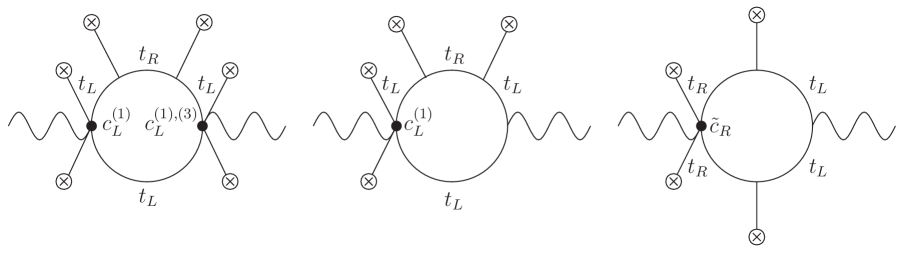
Figure 1: Logarithmic divergent loop diagrams contributing to the SM gauge boson masses, and therefore to $c_{T}$, for the low-energy effective theory of a composite $q_{L}$, Eqs. (11) and (14). The external lines with a cross correspond to insertions of the Higgs VEV.

Now, we must use the renormalization group to scale $c_{T}(M_{q^{*}})$ down to the lower scale $m_{t}$, where we can integrate out the top quark. The leading logarithmic terms arise from the diagrams of Fig. 1. We obtain the equation

$$\xi c_{T}(m_{t})=\xi c_{T}(M_{q^{*}})+\widehat{T}_{top}^{SM}\left(6c_{L}^{2}\xi^{2}+4c_{L}\xi+4\tilde{c}_{R}\epsilon_{t}\right)\log\epsilon_{t}\,.$$ (30)

Finally, we must integrate out the top. The matching condition at the boundary $\mu=m_{t}$ is given by

$$\left[\xi c_{T}(\mu)+\widehat{T}_{top}\right]_{\mu\rightarrow m_{t}^{+}}=\left[\xi c_{T}(\mu)\right]_{\mu\rightarrow m_{t}^{-}}\,,$$ (31)

where in the $\overline{MS}$ scheme

$$\left[\widehat{T}_{top}\right]_{\mu\rightarrow m_{t}^{+}}=\widehat{T}_{top}^{SM}(c_{L}^{2}\xi^{2}+2c_{L}\xi)\,.$$ (32)

Here we are not including the SM top contribution to $c_{T}$ since we want only the contribution to $\widehat{T}$ beyond the one of the SM. Adding up Eqs. (27), (30), and (32) we obtain

$$\widehat{T}=\xi c_{T}(0)=\widehat{T}_{top}^{SM}\left[c_{L}^{2}\xi^{2}\left(\frac{2}{\epsilon_{t}}+7+6\log\epsilon_{t}\right)+c_{L}\xi\left(10+4\log\epsilon_{t}\right)+\epsilon_{t}\left(\frac{22}{3}+4\log\epsilon_{t}\right)\right]\,.$$ (33)

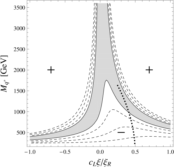
Figure 2: Contribution to $\widehat{T}$ in the $q_{L}$ composite limit (case (a)) in the $M_{q^{*}}-c_{L}\xi/\xi_{R}$ plane, where $\xi_{R}=1/4$. The grey area shows the region $-1.7\cdot 10^{-3}<\widehat{T}<+1.9\cdot 10^{-3}$ and the dashed lines show the contribution to $|\widehat{T}|$ equal to 2.8, 4.2 and 5.6 as they respectively move away from the grey area. We have marked with a “$+$” (“$-$”) the areas in which the contribution to $\widehat{T}$ is positive (negative). The dotted line corresponds to the holographic composite Higgs model.

As explained before, this result is valid in the limit $M_{\rho}\gg M_{q^{*}}\gg m_{t}$. We have checked that in this limit it agrees with the exact calculation.

In Fig. 2 we present a plot of $\widehat{T}$ (the exact result) in the $M_{q^{*}}-c_{L}\xi/\xi_{R}$ plane, where $\xi_{R}=1/4$ is the reference value of $\xi$ in composite Higgs models –see Eq. (4). The grey area shows the region $-1.7\cdot 10^{-3}<\widehat{T}<+1.9\cdot 10^{-3}$ and the dashed lines show the contribution to $|\widehat{T}|$ equal to 2.8, 4.2 and 5.6 as they respectively move away from the grey area; we have marked with a “$+$” (“$-$”) the areas in which the contribution to $\widehat{T}$ is positive (negative). We see that the region of a composite top, $c_{L}\xi/\xi_{R}\sim 1$, is allowed although, as we expected, requires light custodians $M_{q^{*}}\lesssim 1$ TeV. This correlation between $M_{q^{*}}$ and $c_{L}$ tells us that the custodians must be seen at the LHC if $q_{L}$ is a fully composite state. Fig. 2 also shows the region in which $\widehat{T}$ gets a positive contribution, as needed in composite Higgs or Higgsless models in order to satisfy EWPT. We see that a positive contribution $\widehat{T}\sim 1-4\cdot 10^{-3}$ is easily achieved for a composite top, especially for negative values of $c_{L}$ and large values of the custodian mass. For small values of $M_{q^{*}}$, we obtain however a negative value for $\widehat{T}$ that can be easily understood as follows. In the lagrangian Eqs. (23) and (24) the scale $M_{q^{*}}$ is the only breaking parameter of the custodial symmetry. Therefore in the limit $M_{q^{*}}\rightarrow 0$ we must get that the total contribution of the top and custodian sector must be zero, implying that the custodian contribution is given by $\widehat{T}=-\widehat{T}^{SM}_{top}<0$. In Fig. 2 we also show, with a dotted line, the prediction for the holographic Higgs model [10] in which $\xi\sim 1/4$ and $M_{q^{*}}\sim 2.3\sqrt{1-2c_{L}}$ TeV. Notice that in this model the contribution to $\widehat{T}$ is negative, as it is also shown in Ref. [15].

Case (b): In this case the representation of $T_{R}$ is ${\bf(1,3)_{2/3}+(3,1)_{2/3}}$ that implies that the low-energy effective lagrangian for the top and the custodians below $M_{\rho}$ is the same as that of Eqs. (23) and (24) but with $P_{t}^{-1}=\sigma_{3}$. Now the breaking of the custodial symmetry not only comes from the custodian mass term but also from the Yukawa coupling . This implies that, contrary to the case (a), the one-loop contribution to $c_{T}$ is not finite. Indeed, the Yukawa coupling transforms as a $\bf 3$ under the custodial symmetry SU(2)_V, and therefore contributions to $\widehat{T}$ (a $\bf 5$ of SU(2)_V) only need two powers of $y_{t}$. In this case, as shown in Fig. 3, there are custodian diagrams contributing to $\widehat{T}$ that are logarithmically UV-divergent.

We have now $c_{T}(M_{\rho})\propto y_{t}^{2}$ that, being sensitive to the physics at $M_{\rho}$, cannot be predicted within our effective lagrangian approach. What it is calculable, however, is the evolution of the coefficient $c_{T}(\mu)$ from $\mu=M_{\rho}$ to $\mu=M_{q^{*}}$ that comes from the diagrams of Fig. 3.

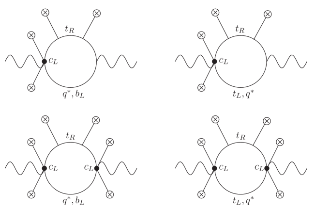
Figure 3: Logarithmic divergent loop diagrams contributing to the SM gauge boson masses, and therefore to $c_{T}$, for the low-energy effective theory of a composite $q_{L}$ and its custodians (case (b)). The external lines with a cross correspond to insertions of the Higgs VEV.

We obtain

$$\xi c_{T}(M_{q^{*}})=\xi c_{T}(M_{\rho})-\widehat{T}_{top}^{SM}16\left(c_{L}^{2}\xi^{2}+c_{L}\xi\right)\log\left(M_{\rho}^{2}/M_{q^{*}}^{2}\right).$$ (34)

From now on we will define $M_{\rho}$ by the scale at which $c_{T}(M_{\rho})=0$. Let us now integrate out the custodians. The coefficients of the effective lagrangian of the top are the same as those in Eq. (25). For $c_{T}$, the matching condition at $\mu=M_{q^{*}}$ reads

$$\left[\xi c_{T}(\mu)\right]_{\mu\rightarrow M_{q^{*}}^{-}}=\left[\xi c_{T}(\mu)+\widehat{T}_{custodians}+\widehat{T}_{mix}\right]_{\mu\rightarrow M_{q^{*}}^{+}}\,,$$ (35)

where

$$\left[\widehat{T}_{custodians}+\widehat{T}_{mix}\right]_{\mu=M_{q^{*}}^{+}}=\widehat{T}_{top}^{SM}\left(2c_{L}^{2}\frac{\xi^{2}}{\epsilon_{t}}+6c_{L}^{2}\xi^{2}-8c_{L}\xi+\frac{22}{3}\epsilon_{t}\right)\,.$$ (36)

Including the evolution of $c_{T}$ from $M_{q^{*}}$ to $m_{t}$ and integrating out the top, that proceeds exactly as in the previous case, we end up with

$$\widehat{T} = \widehat{T}_{top}^{SM}\left[c_{L}^{2}\xi^{2}\left(\frac{2}{\epsilon_{t}}+7+6\log\epsilon_{t}-16\log\frac{M_{\rho}^{2}}{M_{q^{*}}^{2}}\right)\right.$$ (37)

$$+ \left.c_{L}\xi\left(-6+4\log\epsilon_{t}-16\log\frac{M_{\rho}^{2}}{M_{q^{*}}^{2}}\right)+\epsilon_{t}\left(\frac{22}{3}+4\log\epsilon_{t}\right)\right]\,.$$

The exact value of $\widehat{T}$ in the $M_{q^{*}}-c_{L}\xi/\xi_{R}$ plane is presented in Fig. 4 for $M_{\rho}\simeq 2.3$ TeV (left) and $M_{\rho}\simeq 3.6$ TeV (right). The region of sizable values of $c_{L}\xi/\xi_{R}$ is extremely reduced due to the logarithms of Eq. (34), disfavoring the possibility of a composite $q_{L}$ in this case. This analysis, however, is useful to show that regions with positive contributions to $\widehat{T}$ are quite generic; they correspond to $c_{L}<0$. Since previous studies of the effects of $\widehat{T}$ [15] centered in minimal holographic models in which $c_{L}>0$, these regions with positive $\widehat{T}$ were overlooked.

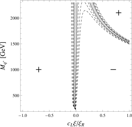
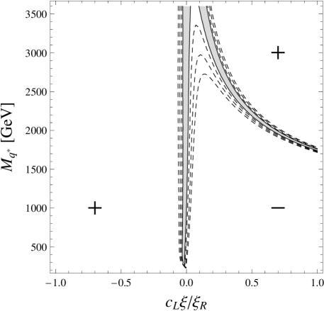
Figure 4: Contribution to $\widehat{T}$ in the $q_{L}$ composite limit (case (b)) in the $M_{q^{*}}-c_{L}\xi/\xi_{R}$ plane, where $\xi_{R}=1/4$. The grey area shows the region $-1.7\cdot 10^{-3}<\widehat{T}<+1.9\cdot 10^{-3}$ and the dashed lines show the contribution to $|\widehat{T}|$ equal to 2.8, 4.2 and 5.6 as they respectively move away from the grey area. We have marked with a “$+$” (“$-$”) the areas in which the contribution to $\widehat{T}$ is positive (negative). We have taken $M_{\rho}=2.3$ TeV (left) and $M_{\rho}=3.6$ TeV (right).

Let us now consider the $t_{R}$ composite limit:

Case (a): In this case $T_{R}$ is a singlet that corresponds, in the limit Eq. (9), to $t_{R}$. There are no custodians and the effective theory below $M_{\rho}$ corresponds to the SM plus the operators of Eqs. (15). We find

$$c_{R}=0\,,$$ (38)

that is a consequence of the custodial symmetry [7]. Eq. (38) together with the absence of custodians imply that $\widehat{T}$ is not generated at the order considered here. Hence, no serious bounds on a composite $t_{R}$ are obtained in this case.

Case (b): In this case $t_{R}\in T_{R}^{(1)}+T_{R}^{(2)}$ transforming as a $(\mathbf{1},\mathbf{3})_{\mathbf{2/3}}+(\mathbf{3},\mathbf{1})_{\mathbf{2/3}}$. There are then five custodians that transform as $\bf 1_{5/3}$, $\bf 1_{-1/3}$ and $\bf 3_{2/3}$ under the electroweak symmetry. Using a $2\times 2$ matrix representation for $T_{R}^{(1),(2)}$, we have the following dimension-4 operators for the top and custodians:

$$\mathcal{L}_{4} = \mathop{\rm Tr}[\bar{T}_{R}^{(1)}i/{D}T_{R}^{(1)}]+\mathop{\rm Tr}[\bar{T}_{R}^{(2)}i/{D}T_{R}^{(2)}]+\mathop{\rm Tr}[\bar{T}_{L}^{(1)}i/{D}T_{L}^{(1)}]+\mathop{\rm Tr}[\bar{T}_{L}^{(2)}i/{D}T_{L}^{(2)}]+\bar{q}_{L}i/{D}q_{L}$$ (39)

$$+ y_{t}\sqrt{2}\mathop{\rm Tr}[(\bar{T}_{R}^{(1)}\Sigma^{\dagger}+\Sigma^{\dagger}\bar{T}_{R}^{(2)})\mathcal{P}_{q}^{-1}(q_{L})]+M_{q^{*}}\left\{\mathop{\rm Tr}[\bar{T}_{R}^{(1)}\widetilde{P}_{t}T_{L}^{(1)}]+\mathop{\rm Tr}[\bar{T}_{R}^{(2)}T_{L}^{(2)}]\right\}+h.c.\,,$$

where $\mathcal{P}_{q}^{-1}(q_{L})=(q_{L},0)$ and $\widetilde{P}_{t}=\sigma_{3}$. These two projectors, appearing in the Yukawa and custodian masses, parametrize the breaking of the custodial symmetry. Contributing to $\widehat{T}$, there can also be dimension-6 operators that, up to order $p^{2}/f^{2}$, are given by

$$\frac{c^{\prime}_{R}}{f^{2}}\left\{\mathop{\rm Tr}\left[\bar{T}^{(1)}_{R}\gamma^{\mu}[\hat{V}_{\mu},T^{(1)}_{R}]\right]-\mathop{\rm Tr}\left[\bar{T}^{(2)}_{R}\gamma^{\mu}[V_{\mu},T^{(2)}_{R}]\right]\right\}\,.$$ (40)

The contribution of the above lagrangian to $c_{T}$ is logarithmically divergent . The divergence is generated by the diagrams of Fig. 5; they give us the evolution of $c_{T}$ from $M_{\rho}$ to $M_{q^{*}}$. Again, choosing the scale $M_{\rho}$ such that $c_{T}(M_{\rho})=0$, we have

$$\xi c_{T}(M_{q^{*}})=-\widehat{T}_{top}^{SM}2c^{\prime\,2}_{R}\xi^{2}\frac{1}{\epsilon_{t}}\log{(M_{\rho}^{2}/M_{q^{*}}^{2})}\,.$$ (41)

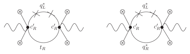
Figure 5: Logarithmic divergent loop diagrams contributing to the SM gauge boson masses, and therefore to $c_{T}$, for the low-energy effective theory of a composite $t_{R}$ and its custodial partners (case (b)). The external lines with a cross correspond to insertions of the Higgs VEV and the crosses denotes $M_{q^{*}}$ insertions.

Let us now integrate the custodians. We are led to the lagrangian Eqs. (15) and (16) with the coefficients

$$c_{R}=0\ ,\quad\tilde{c}_{L}^{(1)}=-\tilde{c}_{L}^{(3)}=\frac{1}{2}\,.$$ (42)

As in the previous case, we have $c_{R}=0$ due to the custodial symmetry [7]. For $c_{T}$, the matching at $\mu=M_{q^{*}}$ is given by Eq. (35) where

$$\left[\widehat{T}_{custodians}+\widehat{T}_{mix}\right]_{\mu\rightarrow M_{q^{*}}^{+}}=\widehat{T}_{top}^{SM}\left(c^{\prime\,2}_{R}\frac{\xi^{2}}{\epsilon_{t}}+4c^{\prime\,2}_{R}\xi^{2}-8c^{\prime}_{R}\xi-\frac{16}{3}\epsilon_{t}\right).$$ (43)

The running from $M_{q^{*}}$ to $m_{t}$ proceeds by the same diagrams as those in Fig. 1 but with the replacements $\tilde{c}_{R}\rightarrow c_{R}\xi/\epsilon_{t}$ and $c_{L}^{(1),(3)}\rightarrow\tilde{c}_{L}^{(1),(3)}\epsilon_{t}/\xi$. We obtain

$$\xi c_{T}(m_{t})=\xi c_{T}(M_{q^{*}})+\widehat{T}_{top}^{SM}\left(-2\epsilon_{t}\right)\log\epsilon_{t}.$$ (44)

Finally, when we match at the top mass scale, Eq. (31), we get

$$\left[\widehat{T}_{top}\right]_{\mu\rightarrow m_{t}^{+}}=\widehat{T}_{top}^{SM}(-\epsilon_{t})\,.$$ (45)

Again, we are not including the SM top contribution. Adding Eqs. (41), (43), (44) and (45), we obtain the total contribution to $\widehat{T}$

$$\widehat{T} =\widehat{T}_{top}^{SM}\left[c^{\prime\,2}_{R}\xi^{2}\left(\frac{1}{\epsilon_{t}}+4-\frac{2}{\epsilon_{t}}\log\frac{M_{\rho}^{2}}{M_{q^{*}}^{2}}\right)-8c^{\prime}_{R}\xi-\epsilon_{t}\left(\frac{19}{3}+2\log\epsilon_{t}\right)\right].$$ (46)

A plot of the value of $\widehat{T}$ is presented in Fig. 6 in the $M_{q^{*}}-c^{\prime}_{R}\xi/\xi_{R}$ plane for $M_{\rho}=2.3$ TeV and $3.6$ TeV. We note that the parameter $c^{\prime}_{R}$ is not related to any coefficient of the low-energy top lagrangian. Nevertheless, since one expects $c^{\prime}_{R}\xi/\xi_{R}$ to be of order $1$ for a composite $t_{R}$, the bounds from Fig. 6 can be considered indirect limits on the degree of compositeness of $t_{R}$. These bounds are strong in the $c^{\prime}_{R}>0$ region, but quite weak for $c^{\prime}_{R}<0$. It is interesting to see that in this latter region it is very natural to have a positive contribution to $\widehat{T}$, as needed for EWPT.

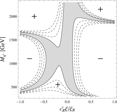
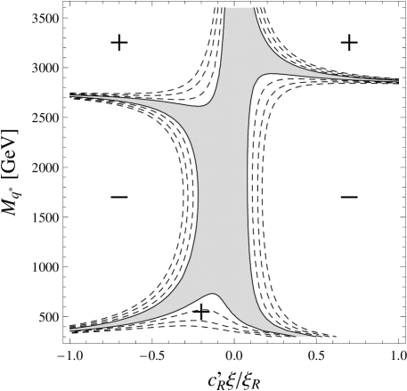
Figure 6: Contribution to $\widehat{T}$ in the $t_{R}$ composite limit (case (b)) in the $M_{q^{*}}-c_{R}^{\prime}\xi/\xi_{R}$ plane, where $\xi_{R}=1/4$. The grey area shows the region $-1.7\cdot 10^{-3}<\widehat{T}<+1.9\cdot 10^{-3}$ and the dashed lines show the contribution to $|\widehat{T}|$ equal to 2.8, 4.2 and 5.6 as they respectively move away from the grey area. We have marked with a “$+$” (“$-$”) the areas in which the contribution to $\widehat{T}$ is positive (negative). We have taken $M_{\rho}=2.3$ TeV (left) and $M_{\rho}=3.6$ TeV (right).

From the above analysis we can summarize the following. A composite $q_{L}$ is only likely in case (a). It yields to $c_{L}^{(1)}=-c_{L}^{(3)}\sim 1$ so it can be tested in modifications of the top couplings. On the other hand, a composite $t_{R}$ is weakly constrained in both cases. Case (a) predicts a small $\widehat{T}$, while in case (b) $\widehat{T}$ can receive sizable positive contributions, and therefore is favored by EWPT. Both cases, however, predict $c_{R}=0$, so the only way to test this possibility is by effects coming from $c_{4t}$ (four-top physics).

4.2 One-loop contributions to $Zb\bar{b}$

Although the coupling $Zb\bar{b}$ is not modified at the tree-level, it can receive corrections at the one-loop level due to loops of SM particles and custodians that break the custodial and $P_{LR}$ symmetry protecting this coupling. Here we only present the one-loop corrections to $Zb_{L}\bar{b}_{L}$ proportional to $c_{4q}$; they are, as we will see, the only one that can be parametrically larger than the corrections to $\widehat{T}$, and then can put, in certain cases, stronger constrains on composite tops . In the limit $M_{\rho}\gg M_{q^{*}}\gg m_{t}$, we find, for the both cases of Eq. (20),

$$\delta g_{b_{L}}=-\delta g_{b_{L}}^{SM}3c_{4q}\xi\left[c_{L}\xi\left(\frac{4}{\epsilon_{t}}\log{\frac{M_{\rho}^{2}}{M_{q^{*}}^{2}}}+4\log{\epsilon_{t}}\right)+2\log{\epsilon_{t}}\right]\,,$$ (47)

where

$$\delta g_{b_{L}}^{SM}=\frac{g}{\cos\theta_{W}}\frac{m_{t}^{2}}{16\pi^{2}v^{2}}\simeq 2\cdot 10^{-3}\,,$$

corresponds to the top one-loop leading-contribution to $Zb\bar{b}$ in the SM. Notice that Eq. (47) shows contributions that grow with the custodian mass and are logarithmically sensitive to the heavy resonance mass $M_{\rho}$. Therefore, for a composite $q_{L}$, where $c_{4q}\sim c_{L}\sim 1$, these contributions to $Zb\bar{b}$ can be larger than those to $\widehat{T}$ for the case (a). For example, for $c_{4q}\sim-1/6$, $c_{L}\sim-0.2$, $\xi\sim 1/4$, and $M_{\rho}\sim 2.3$ TeV, $M_{q^{*}}\sim 800$ GeV, the contributions to $\widehat{T}$ are below the experimental bound but we find $\delta g_{b_{L}}/g_{b_{L}}\sim 0.013$ that is larger than the experimental constraint $-0.002\lesssim\delta g_{b_{L}}/g_{b_{L}}\lesssim 0.006$. These sizable contributions to $Zb\bar{b}$, however, scale with $c_{4q}c_{L}\propto(y_{L}/g_{\rho})^{6}$, while those to $\widehat{T}$ are proportional to $c_{L}^{2}\propto(y_{L}/g_{\rho})^{4}$; therefore the contributions to $Zb\bar{b}$ can be parametrically suppressed with respect to those to $\widehat{T}$ if $y_{L}$ is slightly smaller than $g_{\rho}$. For a composite $t_{R}$, contributions to $Zb\bar{b}$ proportional to the custodian mass or logarithmically sensitive to $M_{\rho}$ are not present, and therefore Fig. 6 will not suffer large modifications.

For very light custodians, the constraints from $Zb\bar{b}$ can be as important as those from $\widehat{T}$ [15, 16]. This implies that the allowed low-$M_{q^{*}}$ regions of Figs. 2 and 6 could be sligthly reduced by the $Zb\bar{b}$ constraints. We leave this calculation for a future publication.

5 Phenomenological implications at future colliders

In this section we want to study the experimental implications of having one of the top chiralities being a composite state. For this purpose, the effective lagrangian of section 3 gives a useful model-independent parametrization of the composite-top new interactions. We will not consider physics involving the Higgs that has been already studied in Ref. [5], and we will only concentrate on top physics.

5.1 Anomalous couplings

The coefficients $c_{L}^{(1),(3)}$ and $c_{R}$ give rise to new contributions to the top coupling to the SM gauge bosons. In particular, for the $Zt_{L}\bar{t}_{L}$, $Wt_{L}\bar{b}_{L}$ and $Zt_{R}\bar{t}_{R}$ couplings, we have respectively

$$\frac{\delta g_{Zt_{L}t_{L}}}{g_{Zt_{L}t_{L}}}=\frac{(c_{L}^{(3)}-c_{L}^{(1)})\xi}{1-\frac{4}{3}\sin^{2}{\theta_{W}}}\ ,\quad\quad\frac{\delta g_{Wt_{L}b_{L}}}{g_{Wt_{L}b_{L}}}=c_{L}^{(3)}\xi\ ,\quad\quad\frac{\delta g_{Zt_{R}t_{R}}}{g_{Zt_{R}t_{R}}}=\frac{3c_{R}\xi}{4\sin^{2}{\theta_{W}}}\,.$$ (48)

In the framework considered here we have $c_{L}^{(3)}\simeq-c_{L}^{(1)}$ and $c_{R}\simeq 0$, and therefore only deviations on the $t_{L}$ couplings can be sizable. To observe these deviations is not going to be easy. At the LHC, top quarks are mostly produced in pairs via the strong gluon fusion process $gg\rightarrow t\bar{t}$, decaying to $Wb$. To measure the $Wt_{L}b_{L}$ coupling, however, a single top must be mostly detected from the process $ub\rightarrow dt$. At the LHC this coupling could be measured with a sensitivity around 7% [17], implying that one could see deviations if $c_{L}\xi\gtrsim 0.07$. For the $Zt\bar{t}$ coupling the situation is more difficult, since it will not be able to be measured at the LHC. The ILC, however, will be the suitable machine to unravel the composite nature of the top. Studies show that the top couplings could be measured with an accuracy as low as 1% [18].

5.1.1 Subleading anomalous coupligs

The operators of section 3 are the dominant ones in a $p^{2}/f^{2}$ expansion. Nevertheless, there are other operators that, although subleading, can have an important impact in future experiments. For a composite $t_{R}$ one of these subleading operators is

$$\frac{ic_{RR}}{f^{2}}\frac{y_{b}}{y_{t}}H^{\dagger}D_{\mu}\widetilde{H}\bar{b}_{R}\gamma^{\mu}t_{R}\,.$$ (49)

where, due to the presence of the $b_{R}$, the coefficient of the operator is suppressed by the Yukawa coupling of the bottom $y_{b}/y_{t}\simeq 0.02$. The coupling $c_{RR}$ is constrained by $b\rightarrow s\gamma$ to be $c_{RR}\xi\lesssim 0.2$ [19]. At the LHC this coupling will be able to be tested in top decays. Ref. [20] gives a precision $-3.2\lesssim c_{RR}\xi\lesssim 6.8$ for an integrated luminosity of $L=10$ fb^-1.

Another subleading operator is

$$\frac{c_{M}y_{t}}{16\pi^{2}f^{2}}\bar{q}_{L}W^{\mu\nu}\widetilde{H}\sigma^{\mu\nu}t_{R}\,,$$ (50)

where $W^{\mu\nu}$ is the field-strenght of the SM $W$ boson. Ref. [20] gives a precision for this coupling at the LHC of order $-3.6\lesssim c_{M}\xi\lesssim 3.6$ for $L=10$ fb^-1. Similar coupling for the gluon could be measured at the LHC with an accuracy $c_{M}\xi\simeq 0.4$ for $L=100$ fb^-1 [17].

5.2 Four-top interactions and $pp\rightarrow t\bar{t}t\bar{t}(b\bar{b})$

The most genuine effect of a composite top comes from the four-top interaction of Eqs. (11) and (15). For a composite $t_{R}$ the operator ${\cal O}_{4t}=(\bar{t}_{R}\gamma^{\mu}t_{R})(\bar{t}_{R}\gamma_{\mu}t_{R})$ induces a top-scattering amplitude that grows with the energy:

$$|{\cal A}(t_{R}\bar{t}_{R}\rightarrow t_{R}\bar{t}_{R})|^{2}=64\frac{c^{2}_{4t}}{f^{4}}(u-2m_{t}^{2})^{2}\,.$$ (51)

Similar expression holds for a composite $t_{L}$, induced in this case by the operator ${\cal O}_{4q}=(\bar{q}_{L}\gamma^{\mu}q_{L})(\bar{q}_{L}\gamma_{\mu}q_{L})$. The growth with the energy of the four-top interaction will lead at the LHC to an enhancement of the cross-section for $pp\rightarrow t\bar{t}t\bar{t}$ as shown in Fig. 7.

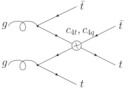
Figure 7: Contribution of the four-top interaction to the process $pp\rightarrow t\bar{t}t\bar{t}$.

We have calculated the total cross-section for the process $pp\rightarrow t\bar{t}t\bar{t}$ using the MadGraph/MadEvent generator [21]. For the computation we have used the CTEQ6M parton distribution functions and $Q=1$ TeV as a reference value of the QCD renormalization and factorization scales. The result as a function of $c_{4t}$ is shown in Fig. 8 for $f=500$ GeV. When the operator ${\cal O}_{4t}$ is generated by a heavy color resonance, Eq. (17), the total cross-section for $pp\rightarrow t\bar{t}t\bar{t}$ is smaller than the SM one. Nevertheless, this cross-section can be substantially larger for larger values of $c_{4t}$. Similar results have been presented previously in Ref. [22].

Figure 8: Cross-section for $pp\rightarrow t\bar{t}t\bar{t}$ as a function of $c_{4t}$ arising from the operator ${\cal O}_{4t}$ (4t), SM diagrams (SM) and both (ALL).

Due to Eq. (51), we expect the $t\bar{t}$ pair coming from the four-top interaction to have a larger invariant mass and transverse momenta than those coming from gluons. Hence, by taking $p_{T}(t_{1})>p_{T}(t_{2})$ (and the same for the anti-tops), we can identify the top $t_{1}$ as the scattered top and the top $t_{2}$ as the spectator top. We also expect the $t_{1}\bar{t}_{1}$ pair to have large invariant mass $m$ and to be produced at large angles and then to have a small pseudorapidity $\eta$. These observables can be useful to discriminate the four-top signal versus backgrounds.

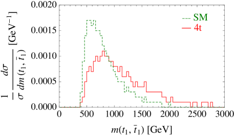
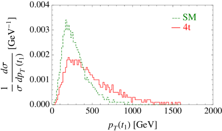
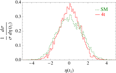
Figure 9: Normalized differential cross-section for $pp\rightarrow t\bar{t}t\bar{t}$ arising from the operator ${\cal O}_{4t}$ and the SM plotted versus the invariant mass of the scattered top pair $m(t_{1},\bar{t}_{1})$, the transverse momentum $p_{T}(t_{1})$, and the pseudorapidity $\eta(t_{1})$.

In Fig. 9 we plot the four-top normalized differential cross-section arising from the four-top contact interaction, and compare this with that of the SM. We show the normalized differential cross-section versus the invariant mass of the scattered top pair $m(t_{1},\bar{t}_{1})$, the transverse momentum of $t_{1}$, $p_{T}(t_{1})$, and its pseudorapidity $\eta(t_{1})$; being normalized distributions, they do not depend on $c_{4t}$ or $f$. As expected, the normalized differential cross-sections due to the new four-top contact interaction are larger for large $m(t_{1},\bar{t}_{1})$, $p_{T}(t_{1})$ or small $\eta(t_{1})$ than those of the SM. In Table 1 we give the values of the cross-section for the four-top production for different cuts in the top-pair invariant-mass, transverse momenta or pseudorapidities. We have taken $c_{4t}=-1/6$ and $f=500$ GeV, corresponding to the values of the composite Higgs model, Eqs. (17) and (4) respectively. For the different cuts we give the value of the significance taken as $\mathcal{S}=\frac{\sigma_{ALL}-\sigma_{SM}}{\sqrt{\sigma_{SM}}}\sqrt{L},$ where $L$ is the integrated luminosity that we take to be $L=100\textnormal{ fb}^{-1}$. We see that the cuts do not substantially increase the significance. Nevertheless, these cuts can be useful in order to eliminate reducible backgrounds, since the detection of the four tops will crucially depend on how well one will be able to reconstruct them at LHC. Since the scattered tops are very energetic, their decay products will be highly collimated, making conventional reconstruction algorithms difficult to apply. In Ref. [22] an analysis at the particle level of the process $pp\rightarrow t\bar{t}t\bar{t}$ has been made, adopting the simple signature of at least two like-sign leptons $l^{\pm}l^{\prime\pm}$ plus at least two hard jets. They get significances $\sim 5$ for a value of $c_{4t}\sim 1/6$ and $f\sim 300-450$ GeV. A more extended analysis at the detector level will be needed to study the feasibility of detecting this process.

	Cuts	$\mathbf{\sigma_{4t}}$[fb]	$\mathbf{\sigma_{SM}}$[fb]	$\mathbf{\sigma_{ALL}}$[fb]	$\mathbf{\mathcal{S}}$
a)	no cuts	1.8	4.6	7.0	11
b)	$m(t_{1},\bar{t}_{1})>650$ GeV	1.5	2.8	4.5	10
c)	$p_{T}(t_{1}),p_{T}(\bar{t}_{1})>200$ GeV, $p_{T}(t_{2}),p_{T}(\bar{t}_{2})>30$ GeV	1.3	2.2	3.5	8.7
d)	$|\eta|(t_{1}),|\eta|(\bar{t}_{1})<2$, $|\eta|(t_{2}),|\eta|(\bar{t}_{2})<4$	1.5	3.5	5.4	10
e)	(b) + (c) + (d)	1.1	1.7	2.8	8.4

Table 1: Cross-section for $pp\rightarrow t\bar{t}t\bar{t}$ arising from ${\cal O}_{4t}$ with $c_{4t}=-1/6$ and $f=500$ GeV (4t), SM diagrams (SM) and both (ALL) for different cuts. The corresponding significance ${\cal S}$ is also given.

	Cuts	$\mathbf{\sigma_{4q}}$[fb]	$\mathbf{\sigma_{SM}}$[fb]	$\mathbf{\sigma_{ALL}}$[fb]	$\mathbf{\mathcal{S}}$
a)	$p_{T}(b),p_{T}(\bar{b})>150$ GeV + $\Delta R(b,\bar{b})>1$	5.6	16	23	18
b)	(a) + $m(t,\bar{t})>600$ GeV	3.9	6.0	11	19
c)	(a) + $m(b,\bar{b})>600$ GeV	3.9	4.4	9.1	23
d)	(a) + $p_{T}(t),p_{T}(\bar{t})>300$ GeV	1.3	1.2	2.6	13

Table 2: Cross-section for $pp\rightarrow t\bar{t}b\bar{b}$ arising from ${\cal O}_{4q}$ with $c_{4q}=-1/6$ and $f=500$ GeV (4q), SM diagrams (SM) and both (ALL) for different cuts. The corresponding significance ${\cal S}$ is also given.

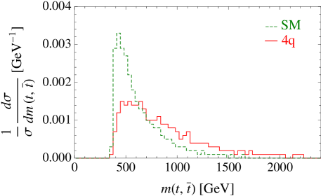
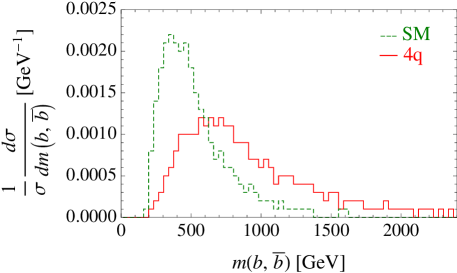
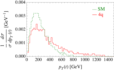
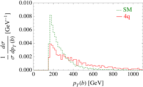
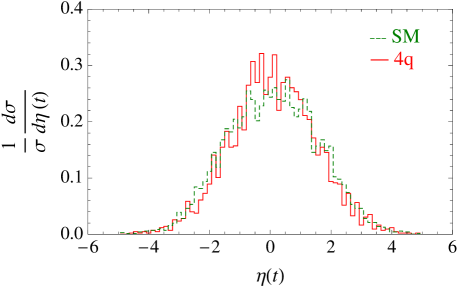
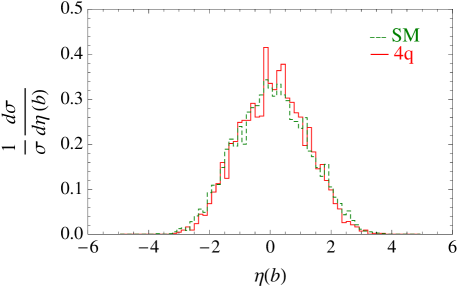
Figure 10: Normalized differential cross-section for $pp\rightarrow t\bar{t}b\bar{b}$ (with cuts $p_{T}(b),p_{T}(\bar{b})>150\,\mathrm{GeV}$ and $\Delta R(b,\bar{b})>1$) induced by the operator ${\cal O}_{4q}$ versus the invariant mass, the transverse momentum and the pseudorapidity of the tops or bottoms. We compare them with those of the SM.

In the case of a composite $q_{L}$, the operator ${\cal O}_{4q}$ also induces an amplitude for the process $b\bar{b}\rightarrow t\bar{t}$ that grows with the energy:

$$|{\cal A}(b_{L}\bar{b}_{L}\rightarrow t_{L}\bar{t}_{L})|^{2}=4\frac{c^{2}_{4q}}{f^{4}}(u-m_{t}^{2}-m_{b}^{2})^{2}\,.$$ (52)

At the LHC this will give an enhancement of the cross-section of $pp\rightarrow t\bar{t}b\bar{b}$ similar to Fig. 7 but with $b$ either as the spectator or the scattered quarks. To calculate with the MadGraph/MadEvent generator the total cross-section for $pp\rightarrow t\bar{t}b\bar{b}$ we will demand a large $p_{T}$ for the bottom quarks and a large separation angle between them, in order to avoid large logarithmic corrections due to collinear $b\bar{b}$ coming from the gluon [23] . In Table 2 we give the cross-section for $pp\rightarrow t\bar{t}b\bar{b}$ for $p_{T}(b),p_{T}(\bar{b})>150$ GeV and $\Delta R(b,\bar{b})=\sqrt{(\eta_{b}-\eta_{\bar{b}})^{2}+(\phi_{b}-\phi_{\bar{b}})^{2}}>1$ where $\phi_{i}$ is the azimuthal angle (we take the renormalization scale $Q=0.5$ TeV, $c_{4q}=-1/6$ and $f=500$ GeV). To show the dependence of the $t\bar{t}b\bar{b}$ production cross-section versus the invariant mass, transverse momentum and pseudorapidity of the bottom and top, we plot in Fig. 10 the normalized differential cross-sections for $pp\rightarrow t\bar{t}b\bar{b}$ induced by the four-fermion interaction, and compare them with the SM ones. The variation of the cross-section and the significance of the signal for several cuts is given in Table 2.

5.2.1 Top polarization measurement

The determination of the top-quark polarization gives a complementary way to probe the properties of the top interactions and to discriminate between either right-handed or left-handed top compositeness. At the LHC, the top quarks are dominantly produced unpolarized by QCD interactions. In the presence of the operators ${\cal O}_{4t,4q}$, however, the $t\bar{t}t\bar{t}$ production yields an excess of either right- or left-handed scattered tops that can be visible by measuring the top polarization.

The polarization of the top quarks can be analyzed from the angular distribution of their decay products. In the decay channel $t\rightarrow W^{+}b\rightarrow l^{+}\nu b,q\bar{q}^{\prime}b$, the angular distribution of the “spin analyzers” $X=l^{+},\nu,q,\bar{q}^{\prime},W^{+},b$ is given by

$$\frac{1}{\Gamma}\frac{d\Gamma}{d\cos{\theta_{X}}}=\frac{1}{2}(1+\alpha_{X}\cos{\theta_{X}})\,,$$ (53)

with $\theta_{X}$ being the angle between the direction of $X$ (in the top rest frame) and the direction of the top polarization. The constants $\alpha_{X}\in[-1,1]$, take in the SM the approximate values $\alpha_{l^{+}}=\alpha_{\bar{d}}=1$, $\alpha_{\nu}=\alpha_{u}=-0.32$, $\alpha_{W^{+}}=-\alpha_{b}=0.41$ [24]. From Eq. (53) we can obtain the top production differential cross-section

$$\frac{1}{\sigma}\frac{d\sigma}{d\cos\theta_{X}}=F_{R}+F_{L}=\frac{A}{2}(1+\alpha_{X}\cos{\theta_{X}})+\frac{1-A}{2}(1-\alpha_{X}\cos{\theta_{X}}),$$ (54)

where $F_{R}$ and $F_{L}$ are respectively the angular distributions for right- and left-handed quarks and $A$ corresponds to the fraction of right-handed quarks produced (therefore $A\in[0,1]$). In the SM we expect $A\sim 1/2$. In Fig. 11 we show the normalized differential cross-section for four-top production at the LHC as a function of $\cos\theta_{X}$ where $X=l^{+}$ is the lepton coming from the top with the highest $p_{T}$. We show this for tops arising either from ${\cal O}_{4t}$ (4t) or ${\cal O}_{4q}$ (4q), and compare with the SM case. By fitting Fig. 11 with the distribution Eq. (54) we find $A\simeq 0.5$ for the SM, while $A\simeq 0.8$ and $0.2$ respectively for the 4t and 4q case. From Eq. (54) one can calculate forward-backward asymmetries in the lepton channel similar to those of Ref. [25] that can be useful to disentangle the helicity of the top if an excess in the four-top production is found at the LHC.

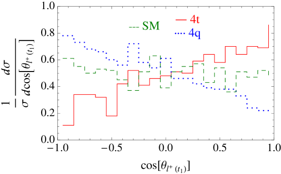
Figure 11: Normalized differential cross-section for $pp\rightarrow t\bar{t}t\bar{t}$ versus $\cos{\theta_{X}}$ where $X$ is the lepton coming from the decay of the scattered top.

6 Conclusions

In models in which EWSB is triggered by a new strong sector or a warped extra dimension, the SM fermions can get their masses by mixing with composite states (or operators) of the new sector. In this framework it is natural to consider due to the heaviness of the top that one of its chiralities, $q_{L}$ or $t_{R}$, is mostly composite.

In this article we have seen that present experimental bounds do not rule out this possibility. The custodial symmetry of the BSM sector plays an important role guaranteeing that the $T$-parameter and $Zb\bar{b}$ do not get corrections at tree-level for the cases (a) and (b) of Eq. (20). We have calculated the one-loop effects to the $T$-parameter and showed, for a composite $q_{L}$, that while in the case (b) the bounds from $\widehat{T}$ are very restrictive (Fig. 4), for the case (a), the presence of the custodial partners of the top, the custodians, avoids large one-loop contributions to $\widehat{T}$ (Fig. 2). For a composite $t_{R}$ the bounds from $\widehat{T}$ are very weak; case (a) does not generate contributions to $\widehat{T}$, while for case (b) one finds wide allowed regions (Fig. 6). Our one-loop calculation shows that moderate and positive contributions to $\widehat{T}$ are more probable in regions in which the coefficients of the higher-dimensional operators $c_{i}$ are negative. These regions, although absent in minimal holographic models [15], can be present in more generic scenarios. These positive contributions to $\widehat{T}$ are needed in this class of models in order to accommodate a generic positive contribution to the $S$-parameter.

At future accelerators, we have seen that top compositeness can be tested by looking for deviations on the $Zt\bar{t}$ and $Wt\bar{b}$ coupling. Only the second one, however, can be measured with certain accuracy at the LHC. The ILC would clearly be an excellent machine to probe the properties of the top and determine its degree of compositeness. A second important effect of top compositeness is the presence of four-top contact terms that enhances the cross-section for $pp\rightarrow t\bar{t}t\bar{t}$ at high-energies. We have calculated the cross-section of this process at the LHC for the case of a composite $t_{R}$, and showed several observables that can allow us to discriminate from the SM prediction. It is however unclear, due to the smallness of the cross-section, whether the four-top production can be seen at the LHC. Clearly, a more detailed analysis is needed to assure the feasibility of this process. Similar analysis has been discussed for the process $pp\rightarrow t\bar{t}b\bar{b}$ for the case of a composite $q_{L}$.

We finalize saying that the composite nature of the top could also be seen indirectly by detecting the custodians. Studies in this direction have been recently carried out in Ref. [26].

References

- [1] S. Weinberg, Phys. Rev. D 13, 974 (1976); Phys. Rev. D 19, 1277 (1979); L. Susskind, Phys. Rev. D 20, 2619 (1979).
- [2] D. B. Kaplan and H. Georgi, Phys. Lett. B 136, 183 (1984); B 136, 187 (1984); M. J. Dugan, H. Georgi and D. B. Kaplan, Nucl. Phys. B 254, 299 (1985).
- [3] C. Csaki, C. Grojean, L. Pilo and J. Terning, Phys. Rev. Lett. 92 (2004) 101802; Y. Nomura, JHEP 0311 (2003) 050; R. Barbieri, A. Pomarol and R. Rattazzi, Phys. Lett. B 591 (2004) 141.
- [4] K. Agashe, R. Contino and A. Pomarol, Nucl. Phys. B 719 (2005) 165.
- [5] G. F. Giudice, C. Grojean, A. Pomarol and R. Rattazzi, JHEP 0706 (2007) 045.
- [6] M. E. Peskin and T. Takeuchi, Phys. Rev. D 46 (1992) 381.
- [7] K. Agashe, R. Contino, L. Da Rold and A. Pomarol, Phys. Lett. B 641 (2006) 62.
- [8] R. Contino, T. Kramer, M. Son and R. Sundrum, JHEP 0705 (2007) 074.
- [9] D. B. Kaplan, Nucl. Phys. B 365 (1991) 259.
- [10] R. Contino, L. Da Rold and A. Pomarol, Phys. Rev. D 75 (2007) 055014.
- [11] R. S. Chivukula, S. B. Selipsky and E. H. Simmons, Phys. Rev. Lett. 69 (1992) 575.
- [12] R. Barbieri, A. Pomarol, R. Rattazzi and A. Strumia, Nucl. Phys. B 703 (2004) 127.
- [13] A. G. Cohen, H. Georgi and B. Grinstein, Nucl. Phys. B 232 (1984) 61.
- [14] D. C. Kennedy, Phys. Lett. B 268 (1991) 86.
- [15] M. S. Carena, E. Ponton, J. Santiago and C. E. M. Wagner, Phys. Rev. D 76 (2007) 035006.
- [16] R. Barbieri, B. Bellazzini, V. S. Rychkov and A. Varagnolo, Phys. Rev. D 76 (2007) 115008; P. Lodone, arXiv:0806.1472 [hep-ph].
- [17] G. Weiglein et al. [LHC/LC Study Group], Phys. Rept. 426 (2006) 47.
- [18] J. A. Aguilar-Saavedra et al. [ECFA/DESY LC Physics Working Group], arXiv:hep-ph/0106315.
- [19] F. Larios, M. A. Perez and C. P. Yuan, Phys. Lett. B 457 (1999) 334.
- [20] J. A. Aguilar-Saavedra, J. Carvalho, N. Castro, F. Veloso and A. Onofre, Eur. Phys. J. C 50 (2007) 519; Eur. Phys. J. C 53 (2008) 689.
- [21] F. Maltoni and T. Stelzer, JHEP 0302 (2003) 027; J. Alwall et al., JHEP 0709 (2007) 028.
- [22] B. Lillie, J. Shu and T. M. P. Tait, JHEP 0804 (2008) 087.
- [23] W. Bernreuther, J. Phys. G 35 (2008) 083001.
- [24] F. Hubaut, E. Monnier, P. Pralavorio, K. Smolek and V. Simak, Eur. Phys. J. C 44S2 (2005) 13.
- [25] K. Agashe, A. Belyaev, T. Krupovnickas, G. Perez and J. Virzi, Phys. Rev. D 77 (2008) 015003.
- [26] R. Contino and G. Servant, arXiv:0801.1679 [hep-ph].