Rational Witt classes of pretzel knots

Abstract.

In his two pioneering articles [5, 6] Jerry Levine introduced and completely determined the algebraic concordance groups of odd dimensional knots. He did so by defining a host of invariants of algebraic concordance which he showed were a complete set of invariants. While being very powerful, these invariants are in practice often hard to determine, especially for knots with Alexander polynomials of high degree. We thus propose the study of a weaker set of invariants of algebraic concordance – the rational Witt classes of knots. Though these are rather weaker invariants than those defined by Levine, they have the advantage of lending themselves to quite manageable computability. We illustrate this point by computing the rational Witt classes of all pretzel knots. We give many examples and provide applications to obstructing sliceness for pretzel knots. Also, we obtain explicit formulae for the determinants and signatures of all pretzel knots.

This article is dedicated to Jerry Levine and his lasting mathematical legacy; on the occasion of the conference “Fifty years since Milnor and Fox”  held at Brandeis University on June 2–5, 2008.

1. Introduction

1.1. Preliminaries

In his seminal papers [5, 6] Jerry Levine introduced and determined the algebraic concordance groups $\mathcal{C}_{n}$ of concordance classes of embeddings of $S^{n}$ into $S^{n+2}$. These groups had previously been found by Kervaire [3] to be trivial for $n$ even; for $n$ odd, Levine proved that

$$\mathcal{C}_{n}\cong\mathbb{Z}^{\infty}\oplus\mathbb{Z}_{2}^{\infty}\oplus\mathbb{Z}_{4}^{\infty}$$

Levine achieved this remarkable result by considering a natural homomorphism $\varphi_{n}:\mathcal{C}_{n}\to\mathcal{I}(\mathbb{Q})$ from the algebraic concordance group $\mathcal{C}_{n}$ into the concordance group of isometric structures $\mathcal{I}(\mathbb{Q})$ on finite dimensional vector spaces over $\mathbb{Q}$ (we describe $\mathcal{I}(\mathbb{Q})$ in detail in section 2.3 below). He constructed a complete set of invariants of concordance of isometric structures and used these invariants to show that $\mathcal{I}(\mathbb{Q})\cong\mathbb{Z}^{\infty}\oplus\mathbb{Z}_{2}^{\infty}\oplus\mathbb{Z}_{4}^{\infty}$. Moreover, he showed that he map $\varphi_{n}:\mathcal{C}_{n}\to\mathcal{I}(\mathbb{Q})$ is injective and that its image is large enough to itself contain a copy of $\mathbb{Z}^{\infty}\oplus\mathbb{Z}_{2}^{\infty}\oplus\mathbb{Z}_{4}^{\infty}$, thereby establishing the isomorphism $\mathcal{C}_{n}\cong\mathbb{Z}^{\infty}\oplus\mathbb{Z}_{2}^{\infty}\oplus\mathbb{Z}_{4}^{\infty}$. In this article we focus exclusively on the case of $n=1$.

To determine the values of Levine’s complete set of invariants for a given knot $K$, one is required to find the irreducible symmetric factors of the Alexander polynomial $\Delta_{K}(t)$ of $K$. As the question of whether or not a given polynomial is irreducible is a difficult one in general, the task of determining all the irreducible factors of a given symmetric polynomial can be quite intractable, more so as the degree of the polynomial grows. To circumnavigate this issue, we consider another homomorphism $\varphi:\mathcal{C}_{1}\to W(\mathbb{Q})$ from the algebraic concordance group $\mathcal{C}_{1}$ into the Witt ring over the rationals ($W(\mathbb{Q})$ is described in detail in section 2.2, for a brief description see section 1.2 below). The isomorphism type of $W(\mathbb{Q})$ as an Abelian group is well understood and is given by $W(\mathbb{Q})\cong\mathbb{Z}\oplus\mathbb{Z}_{2}^{\infty}\oplus\mathbb{Z}_{4}^{\infty}$. The maps $\varphi$ and $\varphi_{1}$ fit into the commutative diagram

From simply knowing the isomorphism types of $\mathcal{C}_{1}$ and $W(\mathbb{Q})$, it is clear that $\varphi:\mathcal{C}_{1}\to W(\mathbb{Q})$ cannot be injective and a loss of information must occurs in passing from $K\in\mathcal{C}_{1}$ to $\varphi(K)\in W(\mathbb{Q})$. The payoff being that one is no longer required to factor polynomials. Indeed, to determine $\varphi(K)$ for a given knot $K\subset S^{3}$ one only needs to use the Gram-Schmidt orthogonalization process along with a simple “reduction”argument (described in section 4.1). The Gram-Schmidt process is completely algorithmic (in contrast with polynomial factorization) and is readily available in many mathematics software packages. To goal of this article then is to underscore the computability and usefulness of the rational Witt classes $\varphi(K)$. Their determination is almost entirely algorithmic and often straightforward, if tedious, to calculate. We illustrate our point by focusing on a concrete family of knots – the set of pretzel knots. This family is large enough to reflect a number of varied properties of the invariant $\varphi$ and yet tractable enough so that a complete determination of the rational Witt classes is possible. We proceed by giving a few details about pretzel knots first and then state our main results.

1.2. Statement of results

Given a positive integer $n$ and integers $p_{1},p_{2},...,p_{n}$, let $P(p_{1},p_{2},...,p_{n})$ denote the $n$-stranded pretzel knot/link. It is obtained by taking $n$ pairs of parallel strands, introducing $p_{i}$ half-twists into the $i$-th strand and capping the strands off by $n$ pairs of bridges. The signs of the $p_{i}$ determine the handedness of the corresponding half-twists. Our convention is that $p_{i}>0$ corresponds to right-handed half-twists, see figure 1 for an example. We limit our considerations to knots and moreover require that $n\geq 3$ and that $p_{i}\neq 0$ (the purpose of these two limitations is to exclude connected sums of torus knots/links). There are 3 categories of choices of the parameters $n,p_{1},...p_{n}$ which lead to knots, namely

(1) $$\mathbf{(i)} n p_{i}$$ is odd and all exept one of the are odd.

(2) $$\mathbf{(ii)} n p_{i}$$ is even and all exept one of the are odd.

(3) $$\mathbf{(iii)} n p_{i}$$ is odd and all are odd.

As we shall see, these categories exhibit slightly different behavior as far as their images in $W(\mathbb{Q})$.

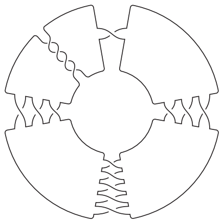
Figure 1. The pretzel knot $P(-1,3,-5,3,4)$.

Pretzel knots are invariant under the action of $\mathbb{Z}_{n}$ by cyclic permutation, i.e. $P(p_{1},p_{2},...,p_{n-1},p_{n})=P(p_{n},p_{1},p_{2},,...,p_{n-1})$. We use this symmetry to fix the convention that if $P(p_{1},...,p_{n})$ comes from either category (i) or (ii) above, we let $p_{n}$ be the unique even integer among $p_{1},...,p_{n}$.

To state our results, we need to give a brief description of the rational Witt ring $W(\mathbb{Q})$, a more copious exposition is provided in section 2.2. As a set, $W(\mathbb{Q})$ consists of equivalence classes of pairs $(\langle\cdot,\cdot\rangle,V)$ where $V$ is a finite dimensional vector space over $\mathbb{Q}$ and $\langle\cdot,\cdot\rangle:V\times V\to\mathbb{Q}$ is a non-degenerate symmetric bilinear form. We say that a pair $(\langle\cdot,\cdot\rangle,V)$ is metabolic or totally isotropic is there exits a half-dimensional subspace $W\subset V$ such that $\langle\cdot,\cdot\rangle|_{W\times W}\equiv 0$. We will be adding pairs $(\langle\cdot,\cdot\rangle_{1},V_{1})$ and $(\langle\cdot,\cdot\rangle_{2},V_{2})$ by direct summing them, thus

$$(\langle\cdot,\cdot\rangle_{1},V_{1})\oplus(\langle\cdot,\cdot\rangle_{2},V_{2})=(\langle\cdot,\cdot\rangle_{1}\oplus\langle\cdot,\cdot\rangle_{2},V_{1}\oplus V_{2})$$

With this understood, the equivalence relation on $W(\mathbb{Q})$ is the one by which $(\langle\cdot,\cdot\rangle_{1},V_{1})$ is equivalent to $(\langle\cdot,\cdot\rangle_{2},V_{2})$ if $(\langle\cdot,\cdot\rangle_{1},V_{1})\oplus(-\langle\cdot,\cdot\rangle_{2},V_{2})$ is metabolic. One proceeds to check that addition is commutative and indeed well defined on $W(\mathbb{Q})$, giving $W(\mathbb{Q})$ the structure of an Abelian group.

It is not hard to obtain an explicit presentation of $W(\mathbb{Q})$ (see theorem 2.1 in section 2.2), for now however it will suffice to point out that $W(\mathbb{Q})$ is generated by the set $\{\langle a\rangle\in W(\mathbb{Q})\,|\,a\in\mathbb{Q}-\{0\}\,\}$. Here $\langle a\rangle$ stands for $(\langle\cdot,\cdot\rangle_{a},\mathbb{Q})$ where $\langle\cdot,\cdot\rangle_{a}$ is the form on $\mathbb{Q}$ specified by $\langle 1,1\rangle_{a}=a$.

Given a knot $K\subset S^{3}$, pick an oriented, genus $g$ Seifert surface $\Sigma\subset S^{3}$ and consider the linking pairing $\ell k:H_{1}(\Sigma;\mathbb{Z})\times H_{1}(\Sigma;\mathbb{Z})\to\mathbb{Z}$ given by

$$\ell k(\alpha,\beta)=\mbox{ linking number between $\alpha$ and $\beta^{+}$ }$$

where $\beta^{+}$ is a small push-off of $\beta$ in the preferred normal direction of $\Sigma$ determined by its orientation. Extending $\ell k$ to $H_{1}(\Sigma;\mathbb{Q})$ linearly and letting $\langle\cdot,\cdot\rangle:H_{1}(\Sigma;\mathbb{Q})\times H_{1}(\Sigma;\mathbb{Q})\to\mathbb{Q}$ be $\langle\alpha,\beta\rangle=\ell k(\alpha,\beta)+\ell k(\beta,\alpha)$, defines a non-degenerate symmetric bilinear pairing on the rational vector space $H_{1}(\Sigma_{g};\mathbb{Q})$. We use this to define

$$\varphi(K)=(\langle\cdot,\cdot\rangle,H_{1}(\Sigma;\mathbb{Q}))\in W(\mathbb{Q})$$

which we refer to as the rational Witt class of $K$. According to [5], $\varphi(K)$ is well defined and only depends on $K$ (as an oriented knot) but not on the particular choice of Seifert surface $\Sigma$. In fact, $\varphi(K)$ only depends on the algebraic concordance class of $K$. With these descriptions out of the way, we are now ready to state our main results.

Theorem 1.1.

Consider category $(i)$ from (1), i.e. let $n\geq 3$ be an odd integer, let $p_{1},...,p_{n-1}$ be odd integers and let $p_{n}\neq 0$ be an even integer. Then the rational Witt class of the pretzel knot $P(p_{1},...,p_{n})$ is given by

$$\varphi(P(p_{1},...,p_{n})) =\bigoplus_{i=1}^{n-1}\left(\left\langle s_{i}\cdot 1\cdot 2\right\rangle\oplus\left\langle s_{i}\cdot 2\cdot 3\right\rangle\oplus...\oplus\left\langle s_{i}\cdot(|p_{i}|-1)\cdot|p_{i}|)\right\rangle\right)\oplus$$

(4) $$\quad\quad\quad\quad\oplus\langle-(p_{1}\cdot...\cdot p_{n-1})\cdot\det P(p_{1},...,p_{n-1})\rangle\oplus$$

(5) $$\quad\quad\quad\quad\oplus\langle\det P(p_{1},...,p_{n-1})\cdot\det P(p_{1},...,p_{n})\rangle$$

where $s_{i}=-Sign(p_{i})$. The two determinants appearing above equal

$$\det P(p_{1},...,p_{n}) =\prod_{i=1}^{n}p_{1}\cdot...\cdot\hat{p}_{i}\cdot...\cdot p_{n}$$

(6) $$\det P(p_{1},...,p_{n-1}) =\prod_{i=1}^{n-1}p_{1}\cdot...\cdot\hat{p}_{i}\cdot...\cdot p_{n-1}$$

As is customary in the literature, having a hat decorate a variable in a product indicates that the factor should be left out. For example $p_{1}\cdot\hat{p}_{2}\cdot p_{3}$ stands for $p_{1}\cdot p_{3}$.

Theorem 1.2.

Consider category $(ii)$ from (1), that is, let $n\geq 3$ be an even integer, let $p_{1},...,p_{n-1}$ be odd integers and let $p_{n}\neq 0$ be an even integer. Then the rational Witt class of the pretzel knot $P(p_{1},...,p_{n})$ is

$$\varphi(P(p_{1},...,p_{n})) =\bigoplus_{i=1}^{n}\left(\left\langle s_{i}\cdot 1\cdot 2\right\rangle\oplus\left\langle s_{i}\cdot 2\cdot 3\right\rangle\oplus...\oplus\left\langle s_{i}\cdot(|p_{i}|-1)\cdot|p_{i}|)\right\rangle\right)\oplus$$

(7) $$\quad\quad\quad\oplus\langle-(p_{1}\cdot...\cdot p_{n})\cdot\det P(p_{1},...,p_{n})\rangle$$

where $s_{i}=-Sign(p_{i})$ and the determinant $\det P(p_{1},...,p_{n})$ is again given by

$$\det P(p_{1},...,p_{n})=\prod_{i=1}^{n}p_{1}\cdot...\cdot\hat{p}_{i}\cdot...\cdot p_{n}$$

To state the next theorem we introduce some auxiliary notation first: Let $\sigma_{j}(t_{1},...,t_{m})$ denote the degree $j$ symmetric polynomial in the variables $t_{1},...,t_{m}$. For example, $\sigma_{1}(t_{1},...,t_{m})=t_{1}+...+t_{m}$ while $\sigma_{m}(t_{1},...,t_{m})=t_{1}\cdot...\cdot t_{m}$. We adopt the convention that $\sigma_{0}(t_{1},...,t_{m})=1$. With this in mind, we have

Theorem 1.3.

Consider category $(iii)$ from (1). Thus, let $n\geq 3$ and $p_{1},...,p_{n}$ be odd integers and let $\sigma_{i}$ stand as an abbreviation for the integer $\sigma_{i}(p_{1},...,p_{i+1})$. Then the rational Witt class of the pretzel knot $P(p_{1},...,p_{n})$ is given by

$$\varphi(P(p_{1},...,p_{n})) =\langle\sigma_{0}\cdot\sigma_{1}\rangle\oplus\langle\sigma_{1}\cdot\sigma_{2}\rangle\oplus...\oplus\langle\sigma_{n-2}\cdot\sigma_{n-1}\rangle$$

We note that $\det P(p_{1},...,p_{n})=\sigma_{n-1}$.

Remark 1.4.

To put the results of theorems 1.1 – 1.3 into perspective, we would like to point out that at the time of this writing, the algebraic concordance orders aren’t known yet even for the 3-stranded pretzel knots $P(p_{1},p_{2},p_{3})$ from category $(i)$ in (1). The chief reason for this is that this family contains knots with Alexander polynomials of arbitrarily high degree.

In contrast, the algebraic concordance orders of $P(p_{1},p_{2},p_{3})$ coming from category $(iii)$ in (1) are well understood and follow easily from Levine’s article [6], see remark 1.12 below. All non-trivial knots in this family are of Seifert genus $1$.

1.3. Applications and examples

While theorems 1.1 – 1.3 give $\varphi(K)$ in terms of the generators of $W(\mathbb{Q})$, in concrete cases one can determine $\varphi(K)$ as a specific element in $\mathbb{Z}\oplus\mathbb{Z}_{2}^{\infty}\oplus\mathbb{Z}_{4}^{\infty}\cong W(\mathbb{Q})$. We give a host of examples of this nature next. Such computations rely on an understanding of the isomorphism between $W(\mathbb{Q})$ and $\mathbb{Z}\oplus\mathbb{Z}_{2}^{\infty}\oplus\mathbb{Z}_{4}^{\infty}$. This isomorphism is completely explicit and easily computed, we explain it in some detail in section 2.2. For now we merely present the results of our computations, the full details are deferred to section 5.

After presenting a several concrete examples, we turn to general type corollaries of theorems 1.1 – 1.3. The ultimate goal of course is to have a set of numerical conditions on $n,p_{1},...,p_{n}$ which would pinpoint the order of $\varphi(K)$ in $W(\mathbb{Q})$. The obstacle to achieving this is number theoretic in nature and we have been unable to overcome it in its full generality. However, we are able to give such conditions for the case of $n=3$ and for some special cases when $n\geq 4$. As we shall see in section 2.2, a necessary condition for $\varphi(K)$ to be zero in $W(\mathbb{Q})$ is that $\sigma(K)=0$ and $|\det K|=m^{2}$ for some odd integer $m$. If only the first of these conditions holds, then $\varphi(K)$ is at least of order $2$ in $W(\mathbb{Q})$. With this in mind the next examples testify that the rational Witt classes carry significantly more information than merely the signature and determinant. We start with a useful definition

Definition 1.5.

If $p$ is an odd integer, we shall say that the knot

$$P(p_{1},...,p_{i-1},p,p_{i},...,p_{j-1},-p,p_{j},...,p_{n})$$

is gotten from $P(p_{1},...,p_{n})$ by an upward stabilization (or conversely that $P(p_{1},...,p_{n})$ is obtained from $P(p_{1},...,p_{i-1},p,p_{i},...,p_{j-1},-p,p_{j},...,p_{n})$ by a downward stabilization).

Example 1.6.

Let $K_{1}$, $K_{2}$ and $K_{3}$ be the knots

$$K_{1}=P(21,13,-17,-15,12)\quad\quad K_{2}=P(-3,-3,-7,5,2)\quad\quad K_{3}=P(-3,-5,7,9,6)$$

from category $(i)$ and let $K=K_{1}\#K_{2}\#K_{3}$. The $\sigma(K)=0$ but $\varphi(K)$ has order $4$ in $W(\mathbb{Q})$. Thus $K$ has concordance order at least $4$. The same holds if $K_{i}$ is replaced by a knot gotten from $K_{i}$ by any finite number of upward stabilizations.

Example 1.7.

Let $K_{1}$ and $K_{2}$ be the knots

$$K_{1}=P(7,3,-5,2)\quad\quad K_{2}=P(-19,-15,21,10)$$

from category $(ii)$ and let $K=K_{1}\#K_{2}$. The $\sigma(K)=0$ but $\varphi(K)$ has order $4$ in $W(\mathbb{Q})$ and therefore also in concordance group. The same is true if $K_{i}$ is replaced by a knot gotten from $K_{i}$ by any finite number of upward stabilizations.

Example 1.8.

Let $K$ be a knot obtained by a finite number of upward stabilization from either

$$P(-3,9,15,-5-5)\quad\mbox{ or }\quad P(-3,-5,-11,15,15)$$

from category $(iii)$. Then the signature of $K$ is zero, the determinant of $K$ is a square but $\varphi(K)\neq 0\in W(\mathbb{Q})$. Consequently, no such $K$ is slice.

Example 1.9.

Let $K_{1}$, $K_{2}$ and $K_{3}$ be the knots

$$K_{1}=P(21,13,-17,-15,12)\quad\quad K_{2}=P(-19,-15,21,10)\quad\quad K_{3}=P(-15,-7,-7,13,11)$$

from the categories $(i)$, $(ii)$ and $(iii)$ and let $K=K_{1}\#K_{2}\#K_{3}$. Then $\sigma(K)=0$ but $\varphi(K)$ is of order $4$ in $W(\mathbb{Q})$. The same holds under replacement of $K_{i}$ by upward stabilizations.

The details of the above computations can be found in section 5. We now turn to more general corollaries of theorems 1.1 – 1.3.

Theorem 1.10.

Consider a 3-stranded pretzel knot $K=P(p,q,r)$ with $p,q,r$ odd. Then the order of $\varphi(K)$ in $W(\mathbb{Q})$ is as follows:

• $\varphi(K)$ is or order 1 in $W(\mathbb{Q})$ if and only if $\det K=-m^{2}$ for some odd $m\in\mathbb{Z}$.

• $\varphi(K)$ is of order 2 in $W(\mathbb{Q})$ if and only if $\det K<0$, $\det K$ is not a square and $|\det K|\equiv 1\,\,(\mbox{mod }4)$.

• $\varphi(K)$ is of order 4 in $W(\mathbb{Q})$ if and only if $\det K<0$ and $|\det K|\equiv 3\,\,(\mbox{mod }4)$.

• $\varphi(K)$ is of infinite order $W(\mathbb{Q})$ if and only if $\det K>0$.

Recall that $\det K=pq+pr+qr$.

Theorem 1.11.

Consider again $K=P(p,q,r)$ but with $p,q$ odd and with $r\neq 0$ even. Then $\varphi(K)$ is of finite order in $W(\mathbb{Q})$ if and only if

$$p+q=0\quad\quad\quad\mbox{ or }\quad\quad\quad p+q=\pm 2\,\,\mbox{ and }\,\,\det K>0$$

The order of $\varphi(K)$ in $W(\mathbb{Q})$ in these cases is as follows:

• If $p+q=0$ then $\varphi(K)$ has order $1$ in $W(\mathbb{Q})$.

• If $p+q=\pm 2$ and $\det K>0$ then

  • $\varphi(K)$ is of order $1$ in $W(\mathbb{Q})$ if $\det K=m^{2}$ for some odd integer $m$.

  • $\varphi(K)$ is of order $2$ in $W(\mathbb{Q})$ if $\det K$ is not a square and is congruent to $1\,(\mbox{mod }4)$.

  • $\varphi(K)$ is of order $4$ in $W(\mathbb{Q})$ if $\det K\equiv 3\,(\mbox{mod }4)$.

Here too $\det K=pq+pr+qr$.

A slightly more general version of this theorem is given in theorem 6.2.

Remark 1.12.

As already mentioned above, the algebraic concordance orders of the knots $P(p,q,r)$ with $p,q,r$ odd are known by work of Levine [6] and agree with the orders of $\varphi(P(p,q,r))$ in $W(\mathbb{Q})$. The analogues of the results of theorem 1.11 are not known for the algebraic concordance group. However, according to theorem 1.15 below, it is clear that when $r$ is even, the order of $\varphi(P(p,q,r))$ in $W(\mathbb{Q})$ and the order of $P(p,q,r)$ in $\mathcal{C}_{1}$ are different in general.

Remark 1.13.

The condition on the congruency class mod $4$, appearing in both theorems 1.11 and 1.10, is reminiscent of a similar condition appearing in a beautiful (and much stronger) theorem by Livingston and Naik [8]: If $K$ is a knot with $\det K=\wp\cdot\beta$ where $\wp$ is a prime congruent to $3$ mod $4$ and $\gcd(\wp,\beta)=1$, then $K$ has infinite order in the topological concordance group.

Theorem 1.14.

Consider a pretzel knot $K=P(p_{1},...,p_{n})$ from category $(i)$ in (1), i.e. assume that $n,p_{1},....,p_{n-1}$ are odd, $n\geq 3$ and $p_{n}\neq 0$ is even. Additionally, suppose that the $p_{1},...,p_{n-1}$ are all mutually coprime. Then $\varphi(K)=0\in W(\mathbb{Q})$ if and only if $\sigma(K)=0$ and $\det K=\pm m^{2}$ for some odd $m\in\mathbb{Z}$.

Seeing as the torsion subgroups of $\mathcal{C}_{1}$ and $W(\mathbb{Q})$ are isomorphic, one can’t help but speculate whether $\varphi|_{Tor(\mathcal{C}_{1})}:Tor(\mathcal{C}_{1})\to W(\mathbb{Q})$ is injective. Unfortunately this is not the case as the next theorem testifies.

Theorem 1.15.

Consider the knot $K=P(5,-3,8)$. All Tristram-Levine signatures $\sigma_{\omega}(K)$ vanish but $K$ is not trivial in $\mathcal{C}_{1}$. On the other hand, the rational Witt class $\varphi(K)$ is zero . Thus, $K$ is a nontrivial element of $\mbox{Ker}(\varphi)\cap Tor(\mathcal{C}_{1})$.

Remark 1.16.

We would like to point out that for knots $K$ with 10 or fewer crossings, $K$ is algebraically slice if and only if $\varphi(K)$ is zero in $W(\mathbb{Q})$. This follows by inspection, using KnotInfo, and relying on the fact that if $\varphi(K)=0$ then $\sigma(K)=0$ and $\det K=\pm m^{2}$.

As a byproduct of our computations we obtain closed formulae for the signature and determinants of all pretzel knots. The formulae for the determinants have already been stated in theorems 1.1 – 1.3, the signature formulae are the content of the next theorem. While these are not directly relevant to our discussion, we list them here in the hopes that they may be useful elsewhere.

Theorem 1.17.

Let $K=P(p_{1},...,p_{n})$ be a pretzel knot from either of the 3 categories $(i)$–$(iii)$ from (1). As usual, we assume that $n\geq 3$. Then the signature $\sigma(K)$ of $K$ can be computed as follows:

1. If $n,p_{1},...,p_{n-1}$ are odd and $p_{n}\neq 0$ is even, then

   $$\sigma(K) =-\left(\sum_{i=1}^{n-1}Sign(p_{i})\cdot(|p_{i}|-1)\right)+Sign(p_{1}\cdot...\cdot p_{n-1}\cdot\det P(p_{1},...,p_{n-1}))+$$

   (8) $$\quad\quad\quad\quad\quad\quad\quad\quad\quad\quad+Sign(\det P(p_{1},...,p_{n-1})\cdot\det P(p_{1},...,p_{n}))$$

   The determinants $\det P(p_{1},...,p_{n})$ and $\det P(p_{1},...,p_{n-1})$ are computed as in theorem 1.1.

2. If $n,p_{n}$ are even, $p_{1},...,p_{n-1}$ are odd and $p_{n}\neq 0$, then

   $$\sigma(K) =-\left(\sum_{i=1}^{n-1}Sign(p_{i})\cdot(|p_{i}|-1)\right)+Sign(p_{1}\cdot...\cdot p_{n}\cdot\det P(p_{1},...,p_{n}))$$

   where $\det P(p_{1},...,p_{n})$ is as computed in theorem 1.2.

3. If $n,p_{1},...,p_{n}$ are all odd, then

   $$\sigma(K) =\sum_{i=1}^{n-1}Sign(\sigma_{i-1}\cdot\sigma_{i})$$

   where $\sigma_{i}=\sigma_{i}(p_{1},...,p_{i+1})$ as in theorem 1.3.

For example, if $K=P(p_{1},...,p_{n})$ with $n,p_{1},...,p_{n}$ odd and $p_{i}>0$ for all $i$, then $\sigma_{i}>0$ for all $i$ also and therefore $\sigma(K)=n-1$. As another example consider the case of $n,p_{n}$ even and $p_{1},...,p_{n-1}$ odd and again $p_{i}>0$ for all $i$. Then $\sigma(K)=n+1-(p_{1}+...+p_{n})$.

1.4. Organization

Section 2 provides background on the three flavors of algebraic concordance groups $\mathcal{C}_{1}$, $\mathcal{I}(\mathbb{Q})$ and $W(\mathbb{Q})$ encountered in the introduction. The relationships between these groups are also made more transparent. In section 3 the first steps towards computing $\varphi(P(p_{1},...,p_{n}))$ are taken in that specific Seifert surfaces are picked for the knots along with specific bases for their first homology. These choices allow us to determined a linking matrix for the knots. Section 4 explains how one can diagonalize the linking matrices found in section 3, leading to proofs of theorems 1.1, 1.2 and 1.3. More detailed versions of these theorems are provided in theorems 4.8, 4.11 and 4.13 respectively. Section 5 is devoted to computations of examples and shows how theorems 1.1 – 1.3 imply the results from examples 1.6 – 1.9 stated above. The final section provides proofs for theorems 1.10, 1.11, 1.14 and 1.15.

Acknowledgement In the preparation of this work I have greatly benefitted from conversations with Chuck Livingston. I am grateful for his generousity in sharing his insight and expertise.

2. Algebraic concordance groups

In this section we describe the three algebraic concordance groups mentioned in the introduction, namely $\mathcal{C}_{1}$ – The algebraic concordance group of classical knots in $S^{3}$. $\mathcal{I}(\mathbb{F})$ – The concordance group of isometric structures over the field $\mathbb{F}$. $W(\mathbb{\mathbb{F}})$ – The Witt ring of non-degenerate, symmetric, bilinear forms over $\mathbb{F}$.

2.1. The algebraic concordance group $\mathcal{C}_{1}$

This section largely follows the exposition from [5] with a slight bias towards a coordinate free description.

Our explanation of the algebraic concordance group $\mathcal{C}_{1}$ runs largely in parallel to the description of the Witt ring $W(\mathbb{Q})$ from the introduction. Thus, we shall consider pairs $(\langle\cdot,\cdot\rangle,L)$ where $L$ is a finitely generated free Abelian group and $\langle\cdot,\cdot\rangle:L\times L\to\mathbb{Z}$ is a bilinear pairing with the property that $\langle\cdot,\cdot\rangle-\langle\cdot,\cdot\rangle^{\tau}$ is unimodular. Following Levine [6], we shall call such pairs admissible pairs. Here $\langle\cdot,\cdot\rangle^{\tau}$ denotes the bilinear form

$$\langle x,y\rangle^{\tau}=\langle y,x\rangle$$

Note that $\langle\cdot,\cdot\rangle$ is not required to be symmetric nor non-degenerate. We will say that $(\langle\cdot,\cdot\rangle,L)$ is metabolic or totally isotropic if there exists a splitting $L\cong L_{1}\oplus L_{2}$ with $rk\,L=2\,(rk\,L_{1})$ and $\langle\cdot,\cdot\rangle|_{L_{1}\times L_{1}}\equiv 0$. We shall add pairs $(\langle\cdot,\cdot\rangle_{1},L_{1})$ and $(\langle\cdot,\cdot\rangle_{2},L_{2})$ by direct summing them, i.e.

$$(\langle\cdot,\cdot\rangle_{1},L_{1})\oplus(\langle\cdot,\cdot\rangle_{2},L_{2})=(\langle\cdot,\cdot\rangle_{1}\oplus\langle\cdot,\cdot\rangle_{2},L_{1}\oplus L_{2})$$

With these definitions understood, we define the algebraic concordance group $\mathcal{C}_{1}$ to be the set of pairs $(\langle\cdot,\cdot\rangle,L)$ as above, up to the equivalence relation $\sim$ by which

$$(\langle\cdot,\cdot\rangle_{1},L_{1})\sim(\langle\cdot,\cdot\rangle_{2},L_{2})\quad\mbox{ if and only if }\quad(\langle\cdot,\cdot\rangle_{1},L_{1})\oplus(-\langle\cdot,\cdot\rangle_{2},L_{2})\mbox{ is metabolic.}$$

We shall refer to this equivalence relation as that of algebraic concordance. Under the operation of direct summing, $\mathcal{C}_{1}$ becomes an Abelian group. An easy check reveals that the inverse of $(\langle\cdot,\cdot\rangle,L)$ is $(-\langle\cdot,\cdot\rangle,L)$. The group $\mathcal{C}_{1}$ was introduced by Jerry Levine in [5] and its isomorphism type was completely determined by him in [6]. The relation of $\mathcal{C}_{1}$ to knot theory is as follows: Let $K$ be a knot in $S^{3}$ and let $\Sigma\subset S^{3}$ be an oriented genus $g$ Seifert surface for $K$. We shall view the orientation on $\Sigma$ as being given by an normal unit vector field $\vec{n}$ on $\Sigma$. Recall from the introduction that the linking pairing $\ell k:H_{1}(\Sigma;\mathbb{Z})\times H_{1}(\Sigma;\mathbb{Z})\to\mathbb{Z}$ is defined by

$$\ell k(x,y)=\mbox{ linking number of $x$ and $y^{+}$ }$$

where, by a customary blurring of viewpoints, we interpret $x$ and $y$ as simple closed curves on $\Sigma$. With this in mind, $y^{+}$ is a small push-off of $y$ in the normal direction of $\Sigma$ determined by $\vec{n}$. It is well known (see e.g. [11]) that $(\ell k,H_{1}(\Sigma;\mathbb{Z}))$ is an admissible pair and therefore the assignment $(K,\Sigma)\mapsto(\ell k,H_{1}(\Sigma;\mathbb{Z}))\in\mathcal{C}_{1}$ is well defined. As Levine shows in [5], the algebraic concordance class of $(\ell k,H_{1}(\Sigma;\mathbb{Z}))$ is independent of $\Sigma$ and by abuse of notation, we shall denote it simply by $K$, hoping that no confusion will arise. Levine also shows that if $K_{1}$ and $K_{2}$ are (geometrically) concordant as knots then their linking forms are algebraically concordant. This statement applies to both smooth and topological (geometric) concordance.

2.2. The Witt ring over the field $\mathbb{F}$

For an excellent introduction to Witt rings we advise the reader to consult [4], but see also [2] and [12]. The first half of this section is a re-iteration of the description for the Witt ring $W(\mathbb{Q})$ over the rational numbers extended to arbitrary fields.

Let $\mathbb{F}$ be a field and consider pairs $(\langle\cdot,\cdot\rangle,V)$ where $V$ is a finite dimensional $\mathbb{F}$-vector space and $\langle\cdot,\cdot\rangle:V\times V\to\mathbb{F}$ is a symmetric, non-degenerate bilinear pairing. By “non-degenerate”  we mean that the map $v\mapsto\langle\cdot,v\rangle$ provides an isomorphism from $V$ to $V^{\ast}$. We call a pair $(\langle\cdot,\cdot\rangle,V)$ metabolic or totally isotropic if there exists a subspace $W\subset V$ with $\dim_{\mathbb{F}}V=2\dim_{\mathbb{F}}W$ and such that $\langle\cdot,\cdot\rangle|_{W\times W}\equiv 0$. As in the case of $\mathbb{F}=\mathbb{Q}$, we define addition of $(\langle\cdot,\cdot\rangle_{1},V_{1})$ and $(\langle\cdot,\cdot\rangle_{2},V_{2})$ by direct sum

$$(\langle\cdot,\cdot\rangle_{1},V_{1})\oplus(\langle\cdot,\cdot\rangle_{2},V_{2})=(\langle\cdot,\cdot\rangle_{1}\oplus\langle\cdot,\cdot\rangle_{2},V_{1}\oplus V_{2})$$

and we proceed to define the equivalence relation $(\langle\cdot,\cdot\rangle_{1},V_{1})\sim(\langle\cdot,\cdot\rangle_{2},V_{2})$ to mean that $(\langle\cdot,\cdot\rangle_{1},V_{1})\oplus(-\langle\cdot,\cdot\rangle_{2},V_{2})$ is metabolic. The set of equivalence classes of pairs $(\langle\cdot,\cdot\rangle,V)$ is denoted by $W(\mathbb{F})$ and called the Witt ring of $\mathbb{F}$. It becomes an Abelian group under the direct sum operation and a commutative ring with the operation of multiplication given by tensor products

$$(\langle\cdot,\cdot\rangle_{1},V_{1})\otimes(\langle\cdot,\cdot\rangle_{2},V_{2})=(\langle\cdot,\cdot\rangle_{1}\cdot\langle\cdot,\cdot\rangle_{2},V_{1}\otimes_{\mathbb{F}}V_{2})$$

The Witt ring $W(\mathbb{F})$ was introduced by Witt in [13] and has found renewed prominence in the theory of quadratic forms over fields through the work of Pfister (see for example [9, 10]).

As is usual in the literature, we will denote $\mathbb{F}-\{0\}$ by $\dot{\mathbb{F}}$. Let us recall the notation $\langle a\rangle$ already used in the introduction: Given $a\in\dot{\mathbb{F}}$ we let $\langle a\rangle$ denote the non-degenerate symmetric bilinear form $(\langle\cdot,\cdot\rangle_{a},\mathbb{F})$ specified by $\langle 1,1\rangle_{a}=a$. Note that

(9) $$\langle a\rangle=\langle a\cdot b^{2}\rangle\in W(\mathbb{F})\quad\forall\,b\in\dot{\mathbb{F}}\quad\quad\mbox{ and }\quad\quad\langle b\rangle\oplus\langle-b\rangle=0\in W(\mathbb{F})\quad\forall b\in\dot{\mathbb{F}}$$

The first of these follows from the fact that $f:(\langle a\rangle,\mathbb{F})\to(\langle a\cdot b^{2}\rangle,\mathbb{F})$ given by $f(x)=x\cdot b$ is an isomorphism of forms. The second form is clearly metabolic and thus zero in $W(\mathbb{F})$. These “harmless”observations are incredibly useful in computations and we will rely on them substantially in our sample calculations in section 5.

With this notation in mind, the following theorem can be found in [4].

Theorem 2.1.

Let $\langle\cdot,\cdot\rangle$ be a non-degenerate symmetric bilinear form on a finite dimensional $\mathbb{F}$-vector space $V$ of dimension $n$. Then there exist scalars $d_{1},...,d_{n}\in\dot{\mathbb{F}}$ such that

$$\langle\cdot,\cdot\rangle=\langle d_{1}\rangle\oplus...\oplus\langle d_{n}\rangle\in W(\mathbb{F})$$

Said differently, $W(\mathbb{F})$ is generated by the set $\{\langle a\rangle\,|\,a\in\dot{\mathbb{F}}\}$. A presentation of $W(\mathbb{F})$ (as a commutative ring) is obtained from these generators along with the relators

$$(R1) \quad\quad\quad\langle 1\rangle-1$$

(10) $$(R2) \quad\quad\quad\langle a\rangle\cdot\langle b\rangle-\langle a\cdot b\rangle a,b\in\dot{\mathbb{F}}$$

(11) $$(R3) \quad\quad\quad\langle a\rangle+\langle b\rangle-\langle a+b\rangle\cdot(1+\langle a\cdot b\rangle) a,b\in\dot{\mathbb{F}}$$

In other words, $W(\mathbb{F})$ is isomorphic to quotient of the free commutative ring generated by the set $\{\langle a\rangle\,|\,a\in\dot{\mathbb{F}}\}$ by the ideal generated by elements of the form as in $(R1)$ – $(R3)$. In $(R1)$, the symbol $1$ denotes the multiplicative unit of $W(\mathbb{F})$.

With this we turn to studying some specific Witt rings. We will chiefly be interested in the cases where $\mathbb{F}$ is either $\mathbb{Q}$ or $\mathbb{F}_{\wp}$ where the latter will be our notation for the finite field of characteristic $\wp\geq 2$. The next result can again be found in [4] and also in [2].

Theorem 2.2.

Let $\wp\in\mathbb{Z}$ be a prime. Then there are isomorphisms of Abelian groups

$$W(\mathbb{F}_{\wp})\cong\left\{\begin{array}[]{cl}\mathbb{Z}_{2}&\quad;\quad\wp=2\cr\mathbb{Z}_{2}\oplus\mathbb{Z}_{2}&\quad;\quad\wp\equiv 1\mbox{ $($mod }4)\cr\mathbb{Z}_{4}&\quad;\quad\wp\equiv 3\mbox{ $($mod }4)\end{array}\right.$$

The generators of $\mathbb{Z}_{2}\cong W(\mathbb{F}_{2})$ and of $\mathbb{Z}_{4}\cong W(\mathbb{F}_{\wp})$ with $\wp\equiv 3\mbox{ $($mod }4)$ are given by $\langle 1\rangle$ while the two copies of $\mathbb{Z}_{2}$ in $W(\mathbb{F}_{\wp})$ in the case when $\wp\equiv 1\mbox{ $($mod }4)$ are generated by $\langle 1\rangle$ and $\langle a\rangle$ where $a\in\dot{\mathbb{F}}$ is any non-square element.

The origins of the proof of the next theorem go back to Gauss’ work on quadratic reciprocity, it was re-discovered by Milnor and Tate [2].

Theorem 2.3.

There is an isomorphism of Abelian groups

$$\sigma\oplus\partial:W(\mathbb{Q})\to\mathbb{Z}\oplus\left(\bigoplus_{\tiny\begin{array}[]{c}\wp\in\mathbb{N}\cr\wp=\mbox{\tiny prime}\end{array}}W(\mathbb{F}_{\wp})\right)$$

where $\sigma:W(\mathbb{Q})\to\mathbb{Z}$ is the signature function while $\partial:W(\mathbb{Q})\to\left(\oplus_{\wp}W(\mathbb{F}_{\wp})\right)$ is the direct sum of homomorphisms $\partial_{\wp}:W(\mathbb{Q})\to W(\mathbb{F}_{\wp})$ (with $\wp$ ranging over all primes) described on generators of $W(\mathbb{F}_{\wp})$ as follows: Given a rational number $\lambda\neq 0$, write it as $\lambda=\wp^{\ell}\cdot\beta$ where $\ell$ is an integer and $\beta$ a rational number whose numerator and denominator are relatively prime to $\wp$. Then

(12) $$\partial_{\wp}(\langle\wp^{\ell}\cdot\beta\rangle)=\left\{\begin{array}[]{cl}0&\quad;\quad\ell\mbox{ is even }\cr\langle\beta\rangle&\quad;\quad\ell\mbox{ is odd }\end{array}\right.$$

Corollary 2.4.

As an Abelian group, $W(\mathbb{Q})$ is isomorphic to $\mathbb{Z}\oplus\mathbb{Z}_{2}^{\infty}\oplus\mathbb{Z}_{4}^{\infty}$.

2.3. The concordance group of isometric structures

For more details on this section, see [6].

Let $\mathbb{F}$ be a field, then an isometric structure over $\mathbb{F}$ is a triple $(\langle\cdot,\cdot\rangle,T,V)$ consisting of a non-degenerate symmetric bilinear form $(\langle\cdot,\cdot\rangle,V)$ and a linear operator $T:V\to V$ which is an isometry with respect to $\langle\cdot,\cdot\rangle$, i.e. $\langle Tv,Tw\rangle=\langle v,w\rangle$ for all $v,w\in V$. A triple $(\langle\cdot,\cdot\rangle,T,V)$ shall be called metabolic or totally isotropic if there is a half-dimensioinal $T$-invariant subspace $W\subset V$ for which $\langle\cdot,\cdot\rangle|_{W\times W}\equiv 0$. Much as in the case of the algebraic concordance group $\mathcal{C}_{1}$ and the Witt ring $W(\mathbb{F})$, isometric structures too are added by direct sum $\oplus$. We define two triples $(\langle\cdot,\cdot\rangle_{1},T_{1},V_{1})$ and $(\langle\cdot,\cdot\rangle_{2},T_{2},V_{2})$ to be equivalent if

$$(\langle\cdot,\cdot\rangle_{1},T_{1},V_{1})\oplus(-\langle\cdot,\cdot\rangle_{2},-T_{2},V_{2})$$

is metabolic. With these definitions understood, we define the concordance group of isometric structures $\mathcal{I}(\mathbb{F})$ as the set of equivalence classes of triples $(\langle\cdot,\cdot\rangle,T,V)$ as above. Not surprisingly, $\mathcal{I}(\mathbb{F})$ becomes an Abelian group under the operation of direct summing.

2.4. Maps between the algebraic concordance groups

Having defined $\mathcal{C}_{1}$, $W(\mathbb{\mathbb{F}})$ and $\mathcal{I}(\mathbb{\mathbb{F}})$, we turn to describing some natural maps between them in the case when $\mathbb{F}=\mathbb{Q}$. We start by a lemma proved by Levine in [6].

Lemma 2.5.

Let $(\langle\cdot,\cdot\rangle,L)$ be an admissible pair (as in section 2.1). Then there exists an admissible pair $(\langle\cdot,\cdot\rangle^{\prime},L^{\prime})$ algebraically concordant to $(\langle\cdot,\cdot\rangle,L)$ and such that $\langle\cdot,\cdot\rangle^{\prime}:L^{\prime}\times L^{\prime}\to\mathbb{Z}$ is a non-degenerate bilinear form.

With this in mind, consider an admissible non-degenerate pair $(\langle\cdot,\cdot\rangle,L)$. Given any basis $\mathcal{B}=\{\alpha_{1},...,\alpha_{n}\}$ of $L$, let $A$ be the matrix representing $\langle\cdot,\cdot\rangle$, that is, set $a_{i,j}=\langle\alpha_{i},\alpha_{j}\rangle$ and let $A=[a_{i,j}]$. We define the maps $\varphi:\mathcal{C}_{1}\to W(\mathbb{Q})$, $\varphi_{1}:\mathcal{C}_{1}\to\mathcal{I}(\mathbb{Q})$ and $\psi:\mathcal{I}(\mathbb{Q})\to W(\mathbb{Q})$ as in [6]

$$\varphi(\langle\cdot,\cdot\rangle,L) =(\langle\cdot,\cdot\rangle+\langle\cdot,\cdot\rangle^{\tau},L\otimes_{\mathbb{Z}}\mathbb{Q})$$

(13) $$\varphi_{1}(\langle\cdot,\cdot\rangle,L) =(A+A^{\tau},-A^{-1}A^{\tau},L\otimes_{\mathbb{Z}}\mathbb{Q})$$

(14) $$\psi(\langle\cdot,\cdot\rangle,T,V) =(\langle\cdot,\cdot\rangle,V)$$

It is not hard to verify that the definition of $\varphi_{1}$ is independent of the choice of the basis $\mathcal{B}$ of $L$. It is also easy to verify that, with respect to $\mathcal{B}$, the matrix $-A^{-1}A^{\tau}$ defines an isometry on $L\otimes_{\mathbb{Z}}\mathbb{Q}$. Is should be clear that $\varphi=\psi\circ\varphi_{1}$, as already pointed out in the introduction. We leave it as an (easy) exercise for the reader to check that these maps are well defined. This requires one to show that metabolic elements from any one group map to metabolic elements in the other groups.

We conclude this section by reminding the reader of the isomorphism types of $\mathcal{C}_{1}$, $W(\mathbb{Q})$ and $\mathcal{I}(\mathbb{Q})$ stated in the introduction:

As already mentioned, Levine showed $\varphi_{1}$ to be injective. Clearly injectivity cannot hold for $\varphi$. However, given the above diagram, one cannot help but ask: “How much loss of information is there if one restricts $\varphi$ to the torsion subgroup of $\mathcal{C}_{1}$?”  As theorem 1.15 shows, the restriction of $\varphi$ to the torsion subgroup of $\mathcal{C}_{1}$ is unfortunately not injective. Nevertheless, examples 1.6 – 1.9 show that $\varphi|_{Tor(\mathcal{C}_{1})}$ contains significantly more information than just the knot determinant.

3. The linking matrices

In this section we compute the linking matrix for $K=P(p_{1},...,p_{n})$ associated to a choice of oriented Seifert surface $\Sigma$ for $K$ along with a concrete basis for $H_{1}(\Sigma;\mathbb{Z})$. The details of these computations for the three cases $(i)$–$(iii)$ from (1) proceed in slightly different manners.

3.1. The case of $n,p_{1},...,p_{n-1}$ odd and $p_{n}$ even

For the remainder of this subsection, we shall assume the conditions from its title with the additional constraints that $n\geq 3$ and $p_{n}\neq 0$.

We start by recalling figure 1 in which we chose a particular projection for the pretzel knot $P(p_{1},...,p_{n})$. We choose $\Sigma_{1}$ to be the Seifert surface for $K$ obtained from that projection via Seifert’s algorithm (see for example [11]). Specifically, $\Sigma_{1}$ consists of $n-1$ disks $D_{1},...,D_{n-1}$ of which $D_{i}$ and $D_{i+1}$ are connected with $|p_{i}|$ bands, each carrying a single half-twist whose handedness is determined by the sign of $p_{i}$ (in that the band obtains a right-handed twist if $p_{i}<0$ and a left-handed twist if $p_{i}>0$). The disks $D_{n-1}$ and $D_{1}$ are similarly connected with $|p_{n-1}|$ bands. Finally, there is a band with $|p_{n}|$ half-twists (right-handed if $p_{n}>0$ and left-handed if $p_{n}<0$) both of whose ends are attached to $D_{1}$. Note that the genus of $\Sigma_{1}$ is $|p_{1}|+|p_{2}|+...+|p_{n-1}|+3-n$.We label the bands connecting $D_{i}$ to $D_{i+1}$ by $B^{i}_{1},...,B^{i}_{|p_{i}|}$ and we label those connecting $D_{n-1}$ to $D_{1}$ by $B^{n-1}_{1},...,B^{n-1}_{|p_{n-1}|}$. The unique band with $|p_{n}|$ twists is labeled $B^{n}$. All of our conventions and labels are illustrated in figure 2.

With these preliminaries in place, we choose our basis

(15) $$\mathcal{B}_{1}=\{\alpha^{1}_{1},...,\alpha^{1}_{|p_{1}|-1},\alpha^{2}_{1},...,\alpha^{2}_{|p_{2}|-1},...,\alpha^{n-1}_{1},...,\alpha^{n-1}_{|p_{n-1}|-1},\gamma,\delta\}$$

for $H_{1}(\Sigma_{1};\mathbb{Z})$ in the following way:

1. We let $\alpha^{i}_{j}$ to be the simple closed curve passing through the bands $B^{i}_{1}$ and$B^{i}_{j+1}$.

2. We pick $\gamma$ to be the simple closed curve passing over the bands $B^{1}_{1}$, $B^{2}_{1}$, …, $B^{n-1}_{1}$.

3. The remaining curve $\delta$ passes once through the band $B^{n}$.

These curves, along with our orientation conventions, are also depicted in figure 2. The orientation of $\Sigma_{1}$ is determined by the normal vector field which points outwards from the page (and towards the reader) on all disks $D_{1},D_{3},D_{5},...$ and into the page (and away from the reader) on the disks $D_{2},D_{4},D_{6},...$ . These conventions are indicated by the symbols $\oplus$ and $\ominus$ respectively in figure 2.

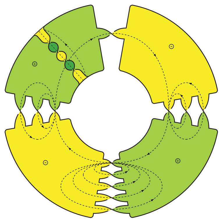
Figure 2. Our choice of Seifert surface $\Sigma_{1}$ for $P(p_{1},...,p_{n})$ for the case when $n,p_{1},...,p_{n-1}$ are odd and $p_{n}$ is even. Our example shows the knot $P(-1,3,-5,3,4)$. The choices of generators for $H_{1}(\Sigma_{1};\mathbb{Z})$ along with their orientations are indicated.

With these definitions in place, we are ready to start computing entries in the linking matrix $\mathcal{L}=[\mathcal{\ell}_{i,j}]$ where $\ell_{i,j}=\ell k(x_{i},x_{j})$. Here $x_{i}$ is the $i$-th element of the basis $\mathcal{B}_{1}$ and $\ell k(x_{i},x_{j})$ is the linking number of $x_{i}$ and $x_{j}^{+}$. The latter is a small push-off of $x_{j}$ in the direction of the normal vector field on $\Sigma_{1}$ determined by its orientation.

Seeing as the loops $\alpha^{i}_{k}$ and $\alpha^{j}_{m}$ are disjoint for any choice of $i\neq j$, we find that $\ell k(\alpha^{i}_{k},\alpha^{j}_{m})=\ell k(\alpha^{j}_{m},\alpha^{i}_{k})=0$ for any choices of $i,j,k,m$ with $i\neq j$. For the same reason, one also obtains $\ell k(\alpha^{i}_{k},\delta)=\ell k(\delta,\alpha^{i}_{k})=0$ for any choices of $i,k$.

The contribution of the subset $\{\alpha^{i}_{1},...,\alpha^{i}_{|p_{i}|-1}\}$ of $\mathcal{B}$ to the linking form $\mathcal{L}$, only depends on $p_{i}$. To see how, let us introduce the $n\times n$ matrices $X_{n}$ and $Y_{n}=X_{n}+X_{n}^{\tau}$ by the formulae

(16) $$X_{n}=\left[\begin{array}[]{rrrrrr}1&0&0&...&0&0\cr 1&1&0&...&0&0\cr 1&1&1&...&0&0\cr\vdots&\vdots&\vdots&\ddots&\vdots&\vdots\cr 1&1&1&...&1&0\cr 1&1&1&...&1&1\cr\end{array}\right]\quad\quad\mbox{ and }\quad\quad Y_{n}=\left[\begin{array}[]{rrrrrr}2&1&1&...&1&1\cr 1&2&1&...&1&1\cr 1&1&2&...&1&1\cr\vdots&\vdots&\vdots&\ddots&\vdots&\vdots\cr 1&1&1&...&2&1\cr 1&1&1&...&1&2\cr\end{array}\right]$$

By consulting figure 2, one finds that

(17) $$\begin{array}[]{ll}\ell k(\alpha^{i}_{k},\alpha^{i}_{m})=\left\{\begin{array}[]{rcl}0&\quad;&k<m\cr-1&\quad;&k\geq m\end{array}\right.&\quad\quad\quad\mbox{ if }p_{i}>0\mbox{ and }i\mbox{ is even.}\cr&\cr\ell k(\alpha^{i}_{k},\alpha^{i}_{m})=\left\{\begin{array}[]{rcl}\phantom{-}1&\quad;&k\leq m\cr 0&\quad;&k>m\end{array}\right.&\quad\quad\quad\mbox{ if }p_{i}<0\mbox{ and }i\mbox{ is even.}\cr&\cr\ell k(\alpha^{i}_{k},\alpha^{i}_{m})=\left\{\begin{array}[]{rcl}-1&\quad;&k\leq m\cr 0&\quad;&k>m\end{array}\right.&\quad\quad\quad\mbox{ if }p_{i}>0\mbox{ and }i\mbox{ is odd.}\cr&\cr\ell k(\alpha^{i}_{k},\alpha^{i}_{m})=\left\{\begin{array}[]{rcl}0&\quad;&k<m\cr\phantom{-}1&\quad;&k\geq m\end{array}\right.&\quad\quad\quad\mbox{ if }p_{i}<0\mbox{ and }i\mbox{ is odd.}\end{array}$$

The case of $p_{i}>0$ and $i$ even is singled out in figure 3.

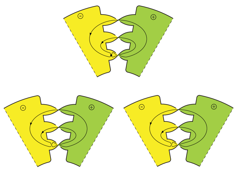
Figure 3. This figure computes the linking $\ell k(\alpha^{i}_{1},\alpha^{i}_{2})$ when $i$ is even. The two push-offs $\alpha^{i,+}_{1}$ and $\alpha^{i,+}_{2}$ of $\alpha^{i}_{1}$ and $\alpha^{i}_{2}$ respectively, are shown in the bottom two pictures. The linking of the two is readily computed from these.

From this we find that $\mathcal{L}_{i}$, the restriction of the linking form $\mathcal{L}$ to the $Span(\alpha^{i}_{1},...,\alpha^{i}_{|p_{i}|-1})$, with respect to the basis $\{\alpha^{i}_{1},...,\alpha^{i}_{|p_{i}|-1}\}$ takes on one of 4 possible forms:

$$\mathcal{L}_{i}=\left\{\begin{array}[]{rl}-X_{|p_{i}|-1}&\quad;\quad\mbox{ if }p_{i}>0\mbox{ and }i\mbox{ is even.}\cr&\cr X^{\tau}_{|p_{i}|-1}&\quad;\quad\mbox{ if }p_{i}<0\mbox{ and }i\mbox{ is even.}\cr&\cr-X^{\tau}_{|p_{i}|-1}&\quad;\quad\mbox{ if }p_{i}>0\mbox{ and }i\mbox{ is odd.}\cr&\cr X_{|p_{i}|-1}&\quad;\quad\mbox{ if }p_{i}<0\mbox{ and }i\mbox{ is odd.}\end{array}\right.$$

In each of the four cases above, the matrix representing $\mathcal{L}_{i}+\mathcal{L}_{i}^{\tau}$ can then be expressed as

(18) $$\mathcal{L}_{i}+\mathcal{L}_{i}^{\tau}=-Sign(p_{i})\,\,Y_{|p_{i}|-1}$$

Having worked out all of the linking numbers $\ell k(\alpha^{i}_{k},\alpha^{j}_{m})$, we now turn to exploring how $\gamma$ and $\delta$ contribute to $\mathcal{L}$. Their linking numbers with the various other curves from the basis $\mathcal{B}$ are easily read off from figure 2:

(19) $$\ell k(\gamma,\gamma) =-(Sign(p_{1})+Sign(p_{2})+...+Sign(p_{n-1}))/2$$

(20) $$\ell k(\gamma,\delta) =0$$

(21) $$\ell k(\delta,\gamma) =1$$

(22) $$\ell k(\delta,\delta) =p_{n}/2$$

while the linking numbers of $\gamma$ with the various $\alpha^{i}_{k}$ are

(23) $$\begin{array}[]{rl}\ell k(\gamma,\alpha^{i}_{k})&=\left\{\begin{array}[]{rr}-1&\quad;\quad\mbox{ if }p_{i}>0\mbox{ and }i\mbox{ is even.}\cr 0&\quad;\quad\mbox{ if }p_{i}<0\mbox{ and }i\mbox{ is even.}\cr 0&\quad;\quad\mbox{ if }p_{i}>0\mbox{ and }i\mbox{ is odd.}\cr 1&\quad;\quad\mbox{ if }p_{i}<0\mbox{ and }i\mbox{ is odd.}\end{array}\right.\cr&\cr\ell k(\alpha^{i}_{k},\gamma)&=\left\{\begin{array}[]{rr}0&\quad;\quad\mbox{ if }p_{i}>0\mbox{ and }i\mbox{ is even.}\cr 1&\quad;\quad\mbox{ if }p_{i}<0\mbox{ and }i\mbox{ is even.}\cr-1&\quad;\quad\mbox{ if }p_{i}>0\mbox{ and }i\mbox{ is odd.}\cr 0&\quad;\quad\mbox{ if }p_{i}<0\mbox{ and }i\mbox{ is odd.}\end{array}\right.\end{array}$$

As earlier, we see that while $\ell k(\alpha^{i}_{k},\gamma)$ and $\ell k(\gamma,\alpha^{i}_{k})$ depend on a number of cases, the quantity $\ell k(\gamma,\alpha^{i}_{k})+\ell k(\alpha^{i}_{k},\gamma)$ always equals $-Sign(p_{i})$. We are thus in a position to assemble all the pieces.

Theorem 3.1.

Let $n,p_{1},...,p_{n-1}$ be odd integers with $n\geq 3$ and let $p_{n}\neq 0$ be an even integer. To keep notation below at bay, let us also introduce the abbreviations

$$s_{i}=-Sign(p_{i})\quad\quad\quad s=s_{1}+...+s_{n-1}\quad\quad\quad\rho_{i}=|p_{i}|-1$$

Then the symmetrized linking form $\mathcal{L}+\mathcal{L}^{\tau}$ of the pretzel knot $P(p_{1},...,p_{n})$ associated to the oriented Seifert surface $\Sigma_{1}$ and the basis

$$\mathcal{B}=\{\alpha^{1}_{1},...,\alpha^{1}_{|p_{1}|-1},\alpha^{2}_{1},...,\alpha^{2}_{|p_{2}|-1},...,\alpha^{n-1}_{1},...,\alpha^{n-1}_{|p_{n-1}|-1},\gamma,\delta\}$$

of $H_{1}(\Sigma_{1};\mathbb{Z})$ as chosen above (see specifically figure 2), has the form

$$\mathcal{L}+\mathcal{L}^{\tau}=\left[\begin{array}[]{ccc|ccc|c|ccc|c|c}&&&&&&\dots&&&&s_{1}&0\cr&s_{1}Y_{\rho_{1}}&&&0&&\dots&&0&&\vdots&\vdots\cr&&&&&&\dots&&&&s_{1}&0\cr\hline\cr&&&&&&\dots&&&&s_{2}&0\cr&0&&&s_{2}Y_{\rho_{2}}&&\dots&&0&&\vdots&\vdots\cr&&&&&&\dots&&&&s_{2}&0\cr\hline\cr\vdots&\vdots&\vdots&\vdots&\vdots&\vdots&\ddots&&&&\vdots&\vdots\cr\hline\cr&&&&&&&&&&s_{n-1}&0\cr&0&&&0&&&&s_{n-1}Y_{\rho_{n-1}}&&\vdots&\vdots\cr&&&&&&&&&&s_{n-1}&0\cr\hline\cr s_{1}&\dots&s_{1}&s_{2}&\dots&s_{2}&\dots&s_{n-1}&\dots&s_{n-1}&s&1\cr\hline\cr 0&\dots&0&0&\dots&0&\dots&0&\dots&0&1&p_{n}\cr\end{array}\right]$$

The matrices $Y_{\rho}$ are as introduced in (16).

3.2. The case of $n$ even, $p_{1},...,p_{n-1}$ odd and $p_{n}$ even

We turn to the next case of choice of parities of $n,p_{1},...,p_{n}$ and pick it for the remainder of this section to be as listed in the title. We also keep our additional assumptions of $n\geq 3$ and $p_{n}\neq 0$.

The Seifert surface $\Sigma_{2}$ that we choose for $P(p_{1},...,p_{n})$ and the preferred basis $\mathcal{B}_{2}$ for $H_{1}(\Sigma_{2};\mathbb{Z})$ are very much like in the case considered in section 3.1. Specifically, we let $\Sigma_{2}$ be obtained from $\Sigma_{1}$ ($\Sigma_{1}$ is the Seifert surface from section 3.1) by simply deleting its unique band with and even number of half-twists and allowing the number of bands which connect the disks $D_{n}$ and $D_{1}$ to be an even number, namley $|p_{n}|$. We then arrive at a surface $\Sigma_{2}$ as in figure 4. The same figure also indicates our choice of basis

$$\mathcal{B}_{2}=\{\alpha^{1}_{1},...,\alpha^{1}_{|p_{1}|-1},\alpha^{2}_{1},...,\alpha^{2}_{|p_{2}|-1},...,\alpha^{n}_{1},...,\alpha^{n}_{|p_{n}|-1},\gamma\}$$

for $H_{1}(\Sigma_{2};\mathbb{Z})$ which is identical to $\mathcal{B}_{1}$ from (15) safe that we are presently no longer requiring the generator $\delta$. The orientation convention is as in the previous section and is again indicated by a $\oplus$ and $\ominus$ in figure 4.

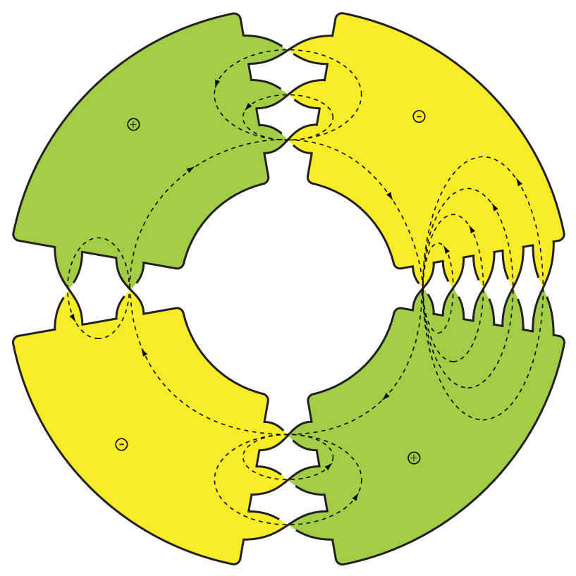
Figure 4. Our choice of Seifert surface $\Sigma_{2}$ for $P(p_{1},...,p_{n})$ for the case when $n$ is even, $p_{1},...,p_{n-1}$ are odd and $p_{n}$ is even. Our example shows the knot $P(3,-5,3,2)$. The choices of generators for $H_{1}(\Sigma_{2};\mathbb{Z})$ with their orientations are indicated.

The linking numbers between the various $\alpha^{i}_{k}$ and $\alpha^{j}_{m}$ and indeed between the $\alpha^{i}_{k}$ and $\gamma$ are identical to those found in section 3.1. We thus immediately arrive at the analogue of theorem 3.1:

Theorem 3.2.

Let $n\geq 3$ be an even integer and let $p_{1},...,p_{n-1}$ be odd integers and $p_{n}\neq 0$ an even integer. Let us re-introduce the abbreviations

$$s_{i}=-Sign(p_{i})\quad\quad\quad s=s_{1}+...+s_{n-1}\quad\quad\quad\rho_{i}=|p_{i}|-1$$

Then the symmetrized linking form $\mathcal{L}+\mathcal{L}^{\tau}$ of the pretzel knot $P(p_{1},...,p_{n})$ associated to the oriented Seifert surface $\Sigma_{2}$ and the basis

$$\mathcal{B}_{2}=\{\alpha^{1}_{1},...,\alpha^{1}_{|p_{1}|-1},\alpha^{2}_{1},...,\alpha^{2}_{|p_{2}|-1},...,\alpha^{n}_{1},...,\alpha^{n}_{|p_{n}|-1},\gamma\}$$

of $H_{1}(\Sigma_{2};\mathbb{Z})$ as chosen above (see specifically figure 4) takes the form

$$\mathcal{L}+\mathcal{L}^{\tau}=\left[\begin{array}[]{ccc|ccc|c|ccc|c}&&&&&&\dots&&&&s_{1}\cr&s_{1}Y_{\rho_{1}}&&&0&&\dots&&0&&\vdots\cr&&&&&&\dots&&&&s_{1}\cr\hline\cr&&&&&&\dots&&&&s_{2}\cr&0&&&s_{2}Y_{\rho_{2}}&&\dots&&0&&\vdots\cr&&&&&&\dots&&&&s_{2}\cr\hline\cr\vdots&\vdots&\vdots&\vdots&\vdots&\vdots&\ddots&&&&\vdots\cr\hline\cr&&&&&&&&&&s_{n}\cr&0&&&0&&&&s_{n}Y_{\rho_{n}}&&\vdots\cr&&&&&&&&&&s_{n}\cr\hline\cr s_{1}&\dots&s_{1}&s_{2}&\dots&s_{2}&\dots&s_{n}&\dots&s_{n}&s\end{array}\right]$$

The matrices $Y_{\rho}$ are as in (16).

3.3. The case of $n$ and $p_{1},...,p_{n}$ odd

In this section we consider the remaining case where all of $n,p_{1},...,p_{n}$ are odd with $n\geq 3$. We start by picking a Seifert surface $\Sigma_{3}$ for $P(p_{1},...,p_{n})$ which is this time obtained by taking two disks and connecting them by $n$ bands $B_{1}$, … $B_{n}$, each with $|p_{i}|$ half twists (right-handed twists if $p_{i}>0$ and left-handed twists if $p_{i}<0$). The thus obtained surface looks as in figure 5.

Figure 5. Our choice of Seifert surface $\Sigma_{3}$ for $P(p_{1},...,p_{n})$ for the case when $n$ and $p_{1},...,p_{n}$ are odd. Our example shows the knot $P(5,-3,3,-3,-1)$. The choices of generators for $H_{1}(\Sigma_{3};\mathbb{Z})$ with their orientations are indicated.

We next choose a basis

$$\mathcal{B}_{3}=\{\alpha_{1},...,\alpha_{n-1}\}$$

of $H_{1}(\Sigma_{3};\mathbb{Z})$ by letting $\alpha_{i}$ be the curve on $\Sigma_{3}$ which runs through the bands $B_{i}$ and $B_{i+1}$. The orientation conventions for the $\alpha_{i}$ and indeed the orientation for $\Sigma_{2}$ itself (indicated again by a $\oplus$ and a $\ominus$) are depicted in figure 5.

The linking form in this basis is rather easy to determine. Note first that $\ell k(\alpha_{i},\alpha_{j})=0$ whenever $|i-j|\geq 2$. On the other hand, by inspection from figure 5, it follows that

$$\ell k(\alpha_{i},\alpha_{i})=\frac{p_{i}+p_{i+1}}{2}\quad\quad\ell k(\alpha_{i},\alpha_{i+1})=-\frac{p_{i+1}+1}{2}\quad\quad\ell k(\alpha_{i+1},\alpha_{i})=-\frac{p_{i+1}-1}{2}$$

With this in place, here is the analogue of theorems 3.1 and 3.2 for the present case.

Theorem 3.3.

Let $n\geq 3$ be an odd integer and let $p_{1},...,p_{n}$ be any odd integers. Then the symmetrized linking form $\mathcal{L}+\mathcal{L}^{\tau}$ of the pretzel knot $P(p_{1},...,p_{n})$ associated to the oriented Seifert surface $\Sigma_{3}$ and the basis $\mathcal{B}_{3}=\{\alpha_{1},...,\alpha_{n-1}\}$ of $H_{1}(\Sigma_{3};\mathbb{Z})$ as chosen above (see figure 5) takes the form

$$\mathcal{L}+\mathcal{L}^{\tau}=\left[\begin{array}[]{cccccccc}p_{1}+p_{2}&-p_{2}&0&0&\dots&0&0&0\cr-p_{2}&p_{2}+p_{3}&-p_{3}&0&\dots&0&0&0\cr 0&-p_{3}&p_{3}+p_{4}&-p_{4}&\dots&0&0&0\cr\vdots&&&\vdots&&&&\vdots\cr 0&0&0&0&\dots&-p_{n-2}&p_{n-2}+p_{n-1}&-p_{n-1}\cr 0&0&0&0&\dots&0&-p_{n-1}&p_{n-1}+p_{n}\end{array}\right]$$

4. Diagonalizing the linking matrices

In this section we show how one can diagonalize the matrices $\mathcal{L}+\mathcal{L}^{\tau}$ obtained in theorems 3.1, 3.2 and 3.3. We do this essentially using the Gram-Schmidt process on $(\langle\cdot,\cdot\rangle,H_{1}(\Sigma;\mathbb{Q}))$ with $\langle x,y\rangle=\ell k(x,y)+\ell k(y,x)$. We need to exercise a bit of care since, while $\langle\cdot,\cdot\rangle$ is non-degenerate, it is by no means definite and square zero vectors do exist.

Once $\mathcal{L}+\mathcal{L}^{\tau}$ has been diagonalized, it is an easy matter to read off the rational Witt class of $\mathcal{L}+\mathcal{L}^{\tau}$ in terms of the generators of $W(\mathbb{Q})$.

4.1. The Gram-Schmidt procedure and reduction

We start by reminding the reader of the Gram-Schmidt process on an arbitrary finite dimensional inner product space $(\langle\cdot,\cdot\rangle,V)$. By convention, such an inner product $\langle\cdot,\cdot\rangle$ is assumed to be positive definite. We then address the issue of square zero vectors in $(\langle\cdot,\cdot\rangle,H_{1}(\Sigma;\mathbb{Q}))$.

Theorem 4.1 (Gram-Schmidt).

Let $\{f_{1},...,f_{n}\}$ be a basis for the inner product space $(\langle\cdot,\cdot\rangle,V)$ and let $\{e_{1},...,e_{n}\}$ be the set of vectors obtained as

$$e_{1} =f_{1}$$

(24) $$e_{2} =f_{2}-\frac{\langle f_{2},e_{1}\rangle}{\langle e_{1},e_{1}\rangle}e_{1}$$

(25) $$e_{3} =f_{3}-\frac{\langle f_{3},e_{2}\rangle}{\langle e_{2},e_{2}\rangle}e_{2}-\frac{\langle f_{3},e_{1}\rangle}{\langle e_{1},e_{1}\rangle}e_{1}$$

(26) $$\vdots$$

(27) $$e_{n} =f_{n}-\frac{\langle f_{n},e_{n-1}\rangle}{\langle e_{n-1},e_{n-1}\rangle}e_{n-1}-...-\frac{\langle f_{n},e_{1}\rangle}{\langle e_{1},e_{1}\rangle}e_{1}$$

Then $\{e_{1},...,e_{n}\}$ is an orthogonal basis for $V$ and $Span\{e_{1},...,e_{i}\}=Span\{f_{1},...,f_{i}\}$ for each $i\leq n$.

Remark 4.2.

In order to keep the scalars in our computations integral (rather than rational and non-integral), we will often use the slightly modified Gram-Schmidt process by which we set

$$e_{i}=d_{i}\cdot\left(f_{i}-\frac{\langle f_{i},e_{i-1}\rangle}{\langle e_{i-1},e_{i-1}\rangle}e_{i-1}-...-\frac{\langle f_{i},e_{1}\rangle}{\langle e_{1},e_{1}\rangle}e_{1}\right)$$

where $d_{i}$ is some common multiple of $\langle e_{1},e_{1}\rangle,...,\langle e_{i-1},e_{i-1}\rangle$. Clearly, the thus created set $\{e_{1},...,e_{n}\}$ is still an orthogonal basis for any choice of $d_{i}\neq 0$.

The next theorem addresses the failure of the Gram-Schmidt procedure in the presence of square zero vectors (on non-definite inner product spaces). The result should be viewed as an iterative prescription to be applied as many times in the Gram-Schmidt process as is the number of square zero vectors $e_{i}$ encountered.

Theorem 4.3.

Let $(\langle\cdot,\cdot\rangle,V)$ be a pair consisting of a finite dimensional $\mathbb{F}$-vector space $V$ and a non-degenerate bilinear symmetric form $\langle\cdot,\cdot\rangle$. Let $\{f_{1},...,f_{n}\}$ be a basis for $V$ and let, for some $m<n$, $\{e_{1},...,e_{m}\}$ be obtained from $\{f_{1},...,f_{n}\}$ as in theorem 4.1 (or alternatively as in remark 4.2). Assume that $\langle e_{i},e_{i}\rangle\neq 0$ for all $i<m$ but that $\langle e_{m},e_{m}\rangle=0$. Additionally, suppose also that $\langle e_{m},f_{m+1}\rangle\neq 0$ (which can always be achieved by a simple reordering, if necessary, of $f_{m+1},...,f_{n}$).

Then $(\langle\cdot,\cdot\rangle,V)$ is equal to $(\langle\cdot,\cdot\rangle^{\prime},V^{\prime})$ in the Witt ring $W(\mathbb{F})$ where

$$V^{\prime}=Span(e_{1},...,e_{m-1},f^{\prime}_{m+2},...,f^{\prime}_{n})\quad\quad\mbox{ and }\quad\quad\langle\cdot,\cdot\rangle^{\prime}=\langle\cdot,\cdot\rangle|_{V^{\prime}\times V^{\prime}}$$

with

$$f^{\prime}_{m+1} =f_{m+1}-\sum_{j=1}^{m-1}\frac{\langle f_{m+1},e_{j}\rangle}{\langle e_{j},e_{j}\rangle}e_{j}$$

(29) $$f^{\prime\prime}_{m+k} =f_{m+k}-\sum_{j=1}^{m-1}\frac{\langle f_{m+k},e_{j}\rangle}{\langle e_{j},e_{j}\rangle}e_{j}$$

(30) $$f^{\prime}_{m+k} =f^{\prime\prime}_{m+k}-\frac{\langle f^{\prime\prime}_{m+k},e_{m}\rangle}{\langle f^{\prime}_{m+1},e_{m}\rangle}f^{\prime}_{m+1}-\frac{\langle f^{\prime\prime}_{m+k},f^{\prime}_{m+1}\rangle\cdot\langle f^{\prime}_{m+1},e_{m}\rangle-\langle f^{\prime\prime}_{m+k},e_{m}\rangle\cdot\langle f^{\prime}_{m+1},f^{\prime}_{m+1}\rangle}{\langle f^{\prime}_{m+1},e_{m}\rangle\cdot\langle f^{\prime}_{m+1},e_{m}\rangle}e_{m}$$

where the last two equations are valid for $k\geq 2$.

Proof.

Let $A$ be the symmetric non-degenerate $n\times n$ matrix representing $\langle\cdot,\cdot\rangle$ with respect to the basis $\{e_{1},...,e_{m-1}\}\cup\{e_{m},f_{m+1},...,f_{n}\}$. Then $A$ is of the form

$$A=\left[\begin{array}[]{ccc|cccc}\langle e_{1},e_{1}\rangle&\dots&0&0&\langle e_{1},f_{m+1}\rangle&...&\langle e_{1},f_{n}\rangle\cr\vdots&\ddots&\vdots&\vdots&\vdots&\ddots&\vdots\cr 0&\dots&\langle e_{m-1},e_{m-1}\rangle&0&\langle e_{m-1},f_{m+1}\rangle&\dots&\langle e_{m-1},f_{m+1}\rangle\cr\hline\cr 0&\dots&0&0&\langle e_{m},f_{m+1}\rangle&...&\langle e_{m},f_{n}\rangle\cr\langle f_{m+1},e_{1}\rangle&\dots&\langle f_{m+1},e_{m-1}\rangle&\langle f_{m+1},e_{m}\rangle&\langle f_{m+1},f_{m+1}\rangle&...&\langle f_{m+1},f_{n}\rangle\cr\vdots&\ddots&\vdots&\vdots&\vdots&\ddots&\vdots\cr\langle f_{n},e_{1}\rangle&\dots&\langle f_{n},e_{m-1}\rangle&\langle f_{n},e_{m}\rangle&\langle f_{n},f_{m+1}\rangle&...&\langle f_{n},f_{n}\rangle\end{array}\right]$$

For $k\geq 1$, let $f^{\prime\prime}_{m+k}$ be given by

$$f^{\prime\prime}_{m+k}=f_{m+k}-\sum_{j=1}^{m-1}\frac{\langle f_{m+k},e_{j}\rangle}{\langle e_{j},e_{j}\rangle}e_{j}$$

so that $\langle f^{\prime\prime}_{m+k},e_{i}\rangle=0$ for all $k\geq 1$ and all $i\leq m-1$. Thus the matrix $A^{\prime\prime}$ representing $\mathcal{L}+\mathcal{L}^{\tau}$ with respect to the basis $\{e_{1},...e_{m},f^{\prime\prime}_{m+1},...,f^{\prime\prime}_{n}\}$ looks like

$$A^{\prime\prime}=\left[\begin{array}[]{ccc}\langle e_{1},e_{1}\rangle&\dots&0\cr\vdots&\ddots&\vdots\cr 0&\dots&\langle e_{m-1},e_{m-1}\rangle\end{array}\right]\oplus\left[\begin{array}[]{cccc}0&\langle e_{m},f_{m+1}\rangle&...&\langle e_{m},f_{n}\rangle\cr\langle f_{m+1},e_{m}\rangle&\langle f^{\prime\prime}_{m+1},f^{\prime\prime}_{m+1}\rangle&...&\langle f^{\prime\prime}_{m+1},f^{\prime\prime}_{n}\rangle\cr\vdots&\vdots&\ddots&\vdots\cr\langle f_{n},e_{m}\rangle&\langle f^{\prime\prime}_{n},f^{\prime\prime}_{m+1}\rangle&...&\langle f^{\prime\prime}_{n},f^{\prime\prime}_{n}\rangle\end{array}\right]$$

Note that $\langle e_{m},f^{\prime\prime}_{m+k}\rangle=\langle e_{m},f_{m+k}\rangle$ for all $k\geq 1$. To simplify the second summand, we introduce a further change of basis by setting

$$f^{\prime}_{m+k}=f^{\prime\prime}_{m+k}-\frac{\langle f^{\prime\prime}_{m+k},e_{m}\rangle}{\langle f^{\prime\prime}_{m+1},e_{m}\rangle}f^{\prime\prime}_{m+1}-\frac{\langle f^{\prime\prime}_{m+k},f^{\prime\prime}_{m+1}\rangle\cdot\langle f^{\prime\prime}_{m+1},e_{m}\rangle-\langle f^{\prime\prime}_{m+k},e_{m}\rangle\cdot\langle f^{\prime\prime}_{m+1},f^{\prime\prime}_{m+1}\rangle}{\langle f^{\prime\prime}_{m+1},e_{m}\rangle\cdot\langle f^{\prime\prime}_{m+1},e_{m}\rangle}e_{m}$$

for all $k\geq 2$ and for convenience, set $f^{\prime}_{m+1}=f^{\prime\prime}_{m+1}$. A quick check reveals that now

$$\langle f^{\prime}_{m+k},e_{m}\rangle=0\quad\quad\mbox{ and }\quad\quad\langle f^{\prime}_{m+k},f^{\prime}_{m+1}\rangle=0\quad\quad\forall k\geq 2$$

Therefore the second summand of $A^{\prime\prime}$ above, when expressed with respect to the basis $\{e_{m},f^{\prime}_{m+1},...,f^{\prime}_{n}\}$, takes the form

$$\left[\begin{array}[]{cc}0&\langle e_{m},f_{m+1}\rangle\cr\langle f_{m+1},e_{m}\rangle&\langle f^{\prime}_{m+1},f^{\prime}_{m+1}\rangle\end{array}\right]\oplus\left[\begin{array}[]{ccc}\langle f^{\prime}_{m+2},f^{\prime}_{m+2}\rangle&...&\langle f^{\prime}_{m+2},f^{\prime}_{n}\rangle\cr\vdots&&\vdots\cr\langle f^{\prime}_{n},f^{\prime}_{m+2}\rangle&...&\langle f^{\prime}_{n},f^{\prime}_{n}\rangle\end{array}\right]$$

Since the first summand is metabolic and therefore equals zero in $W(\mathbb{F})$, the claim of the theorem follows. ∎

We shall refer to the passage from $(\langle\cdot,\cdot\rangle,V)$ to $(\langle\cdot,\cdot\rangle^{\prime},V^{\prime})$, as described in theorem 4.3, as reduction, seeing as the dimension of $V$ gets reduced by $2$ in the process.

4.2. The case of $n,p_{1},...,p_{n-1}$ odd and $p_{n}$ even, revisited

The goal of this subsection is to diagonlize the symmetrized linking matrix $\mathcal{L}+\mathcal{L}^{\tau}$ obtained in theorem 3.1. Specifically, we want to find a regular matrix $P$ of the same dimension as $\mathcal{L}+\mathcal{L}^{\tau}$ such that $P^{\tau}(\mathcal{L}+\mathcal{L}^{\tau})P$ is a diagonal matrix. By way of shortcut of notation, we will write $\langle x,y\rangle$ to denote $\ell k(x,y)+\ell k(y,x)$.

As the matrix $\mathcal{L}+\mathcal{L}^{\tau}$ from theorem 3.1 consists of a number of matrix blocks of the form $\pm Y_{m}$ (see (16) for the definition of $Y_{m}$), we first take the time to apply the Gram-Schmidt process to the latter. We let $P_{m}$ denote the upper triangular $m\times m$ matrix given by

(31) $$P_{m}=\left[\begin{array}[]{rrrrrrr}1&-1&-1&-1&...&-1&-1\cr 0&2&-1&-1&...&-1&-1\cr 0&0&3&-1&...&-1&-1\cr\vdots&\vdots&\vdots&\vdots&\vdots&\vdots&\vdots\cr 0&0&0&&...&m-1&-1\cr 0&0&0&&...&0&m\cr\end{array}\right]$$

Lemma 4.4.

Consider the inner product space $(\langle\cdot,\cdot\rangle,\mathbb{Z}^{m})$ where the inner product $\langle\cdot,\cdot\rangle$ with respect to the standard basis $\{\alpha_{1},...,\alpha_{m}\}$ of $\mathbb{Z}^{m}$ is given by

$$\langle\alpha_{i},\alpha_{j}\rangle=(i,j)\mbox{--th entry of the matrix }Y_{m}\mbox{ from \eqref{X-n}}$$

Then defining $a_{i}=i\alpha_{i}-\alpha_{i-1}-\alpha_{i-2}-...-\alpha_{1}$ for each $i=1,...,m$ yields an orthogonal basis for $(\langle\cdot,\cdot\rangle,\mathbb{Z}^{m})$ with $\langle a_{i},a_{i}\rangle=i(i+1)$. Said differently,

$$P_{m}^{\tau}\,Y_{m}\,P_{m}=\mbox{Diag}\,(1\cdot 2\,,\,2\cdot 3\,,\,3\cdot 4\,,...,\,m\cdot(m+1))$$

Proof.

This is a straightforward application of the Gram-Schmidt process. Let $a_{i}$ be as stated in the lemma and assume that $\{a_{1},...,a_{i}\}$ is an orthogonal set for all $i<k\leq m$ with the stated squares $\langle a_{i},a_{i}\rangle=i(i+1)$ (the case of $i=1$ being clearly true). We prove that the statement remains true if $i$ is chosen to be $k$. Note that

$$\langle\alpha_{k},a_{i}\rangle=\langle\alpha_{k},i\alpha_{i}-\alpha_{i-1}-...-\alpha_{1}\rangle=i-1-1-...-1=1$$

for any choice of $i<k$. Using the Gram-Schmidt process gives

$$a_{k} =\alpha_{k}-\frac{\langle\alpha_{k},a_{k-1}\rangle}{\langle a_{k-1},a_{k-1}\rangle}a_{k-1}-...-\frac{\langle\alpha_{k},a_{1}\rangle}{\langle a_{1},a_{1}\rangle}a_{1}$$

(32) $$=\alpha_{k}-\frac{1}{(k-1)k}((k-1)\alpha_{k-1}-\alpha_{k-2}-...-\alpha_{1})-...-\alpha_{1}$$

(33) $$=\frac{1}{k}\left(k\alpha_{k}-\alpha_{k-1}-\alpha_{k-2}-...-\alpha_{1}\right)$$

Proceeding as in remark 4.2, we let $a_{k}$ be equal to

$$a_{k}=k\alpha_{k}-\alpha_{k-1}-\alpha_{k-2}-...-\alpha_{1}$$

which already showes that $\{a_{1},...,a_{k}\}$ is orthogonal. To complete the proof of the lemma, we need to compute $\langle a_{k},a_{k}\rangle$:

$$\langle a_{k},a_{k}\rangle =\langle k\alpha_{k}-\alpha_{k-1}-...-\alpha_{1},k\alpha_{k}-\alpha_{k-1}-...-\alpha_{1}\rangle$$

(37) $$=k^{2}\langle\alpha_{k},\alpha_{k}\rangle-2k\langle\alpha_{k},\alpha_{k-1}+...+\alpha_{1}\rangle+\sum_{i=1}^{k-1}\langle\alpha_{i},\alpha_{i}\rangle+\sum_{\tiny\begin{array}[]{c}i,j=1\cr i\neq j\end{array}}^{k-1}\langle\alpha_{i},\alpha_{j}\rangle$$

(38) $$=2k^{2}-2k(k-1)+2(k-1)+((k-1)^{2}-(k-1))$$

(39) $$=k(k+1)$$

which is as claimed. ∎

We proceed by defining vectors $a^{i}_{k}$ as

$$a^{i}_{k}=k\alpha^{i}_{k}-\alpha^{i}_{k-1}-...-\alpha^{i}_{1}$$

for each $i=1,...,n-1$. Lemma 4.4 then shows that for each such index $i$, the set $\{a^{i}_{1},...,a^{i}_{|p_{i}|-1}\}$ is an orthogonal set with respect to $\langle\cdot,\cdot\rangle=\mathcal{L}+\mathcal{L}^{\tau}$ and $\langle a^{i}_{k},a^{i}_{k}\rangle=-Sign(p_{i})\,k(k+1)$. Moreover, since $\langle\alpha^{i}_{k},\alpha^{j}_{m}\rangle=0$ whenever $i\neq j$, we see that in fact the set

(40) $$\mathcal{B}^{\perp}_{1,prelim}=\{a^{1}_{1},...,a^{1}_{|p_{1}|-1},a^{2}_{1},...,a^{2}_{|p_{2}|-1},...,a^{n-1}_{1},...,a^{n-1}_{|p_{n-1}|-1}\}$$

is also an orthogonal set.

We then turn to finding two additional vectors, which we shall label $X$ and $Y$, needed to complete $\mathcal{B}^{\perp}_{1,prelim}$ to an orthogonal basis for $\mathcal{B}_{1}^{\perp}$ for $H_{1}(\Sigma_{1};\mathbb{Q})$. We find $X$ using again the Gram-Schmidt process.

Lemma 4.5.

Setting $X$ equal to

$$X=|p_{1}\cdot...\cdot p_{n-1}|\,\gamma-\sum_{i=1}^{n-1}\left(\left(\prod_{k\neq i}|p_{k}|\right)\sum_{k=1}^{|p_{i}|-1}\alpha^{i}_{k}\right)$$

makes the set $\mathcal{B}^{\perp}_{1,prelim}\cup\{X\}$ an orthogonal set. Moreover, the square of $X$ is

$$\langle X,X\rangle=-(p_{1}\cdot...\cdot p_{n-1})^{2}\left(\frac{1}{p_{1}}+...+\frac{1}{p_{n-1}}\right)$$

Proof.

An easy induction argument on $|p_{i}|$ shows that

$$\sum_{k=1}^{|p_{i}|-1}\frac{\langle\gamma,a^{i}_{k}\rangle}{\langle a^{i}_{k},a^{i}_{k}\rangle}a^{i}_{k}=\frac{1}{|p_{i}|}(\alpha^{i}_{1}+\alpha^{i}_{2}+...+\alpha^{i}_{|p_{i}|-1})$$

Letting $X$ be given by the Gram-Schmidt formula

$$X=\gamma-\sum_{i=1}^{n-1}\sum_{k=1}^{|p_{i}|-1}\frac{\langle\gamma,a^{i}_{k}\rangle}{\langle a^{i}_{k},a^{i}_{k}\rangle}a^{i}_{k}$$

leads, in conjunction with the above formula, to

$$X=\gamma-\sum_{i=1}^{n-1}\frac{1}{|p_{i}|}\sum_{k=1}^{|p_{i}|-1}\alpha^{i}_{k}$$

To keep coefficients integral (see remark 4.2) we multiply the right-hand side of the above by $|p_{1}\cdot...\cdot p_{n-1}|$ and set $X$ instead equal to

$$X=|p_{1}\cdot...\cdot p_{n-1}|\,\gamma-\sum_{i=1}^{n-1}\left(\left(\prod_{k\neq i}|p_{k}|\right)\sum_{k=1}^{|p_{i}|-1}\alpha^{i}_{k}\right)$$

as in the statement of the lemma. Thus, $\mathcal{B}^{\perp}_{1,prelim}\cup\{X\}$ is indeed an orthogonal set.

We next compute $\langle X,X\rangle$:

$$\langle X,X\rangle =(p_{1}\cdot...\cdot p_{n-1})^{2}\langle\gamma,\gamma\rangle+\sum_{i=1}^{n-1}\left[\left(\prod_{k\neq i}|p_{k}|\right)^{2}\left\langle\sum_{k=1}^{|p_{i}|-1}\alpha^{i}_{k},\sum_{k=1}^{|p_{i}|-1}\alpha^{i}_{k}\right\rangle\right]-$$

(41) $$-2\sum_{i=1}^{n-1}\frac{(p_{1}\cdot...\cdot p_{n-1})^{2}}{|p_{i}|}\left\langle\gamma,\sum_{k=1}^{|p_{i}|-1}\alpha^{i}_{k}\right\rangle$$

Using the linking form $\mathcal{L}$ from theorem 3.1, it is easy to see that (for example by induction on $|p_{i}|$)

$$\left\langle\sum_{k=1}^{|p_{i}|-1}\alpha^{i}_{k},\sum_{k=1}^{|p_{i}|-1}\alpha^{i}_{k}\right\rangle =-Sign(p_{i})\,|p_{i}|\,(|p_{i}|-1)$$

(42) $$\left\langle\gamma,\sum_{k=1}^{|p_{i}|-1}\alpha^{i}_{k}\right\rangle =-Sign(p_{i})\,(|p_{i}|-1)$$

which in turn shows that

$$\sum_{i=1}^{n-1} \left[\left(\prod_{k\neq i}|p_{k}|\right)^{2}\left\langle\sum_{k=1}^{|p_{i}|-1}\alpha^{i}_{k},\sum_{k=1}^{|p_{i}|-1}\alpha^{i}_{k}\right\rangle\right]-2\sum_{i=1}^{n-1}\frac{(p_{1}\cdot...\cdot p_{n-1})^{2}}{|p_{i}|}\left\langle\gamma,\sum_{k=1}^{|p_{i}|-1}\alpha^{i}_{k}\right\rangle=$$

(43) $$=- \sum_{i=1}^{n-1}Sign(p_{i})\frac{(p_{1}\cdot...\cdot p_{n-1})^{2}}{|p_{i}|}(|p_{i}|-1)+2\sum_{i=1}^{n-1}Sign(p_{i})\frac{(p_{1}\cdot...\cdot p_{n-1})^{2}}{|p_{i}|}(|p_{i}|-1)$$

(44) $$= \sum_{i=1}^{n-1}Sign(p_{i})\frac{(p_{1}\cdot...\cdot p_{n-1})^{2}}{|p_{i}|}(|p_{i}|-1)$$

(45) $$= |p_{1}\cdot...\cdot p_{n-1}|\,\sum_{i=1}^{n-1}Sign(p_{i})\left(\prod_{k\neq i}|p_{k}|\right)(|p_{i}|-1)$$

Finally, recalling (see theorem 3.1) that $\langle\gamma,\gamma\rangle=-(Sign(p_{1})+...+Sign(p_{n-1}))$, we are able to assemble all the pieces to compute $\langle X,X\rangle$:

$$\frac{1}{|p_{1}\cdot...\cdot p_{n-1}|}\,\langle X,X\rangle =-|p_{1}\cdot...\cdot p_{n-1}|(Sign(p_{1})+...+Sign(p_{n-1}))+$$

(46) $$\quad\quad\quad\quad+\sum_{i=1}^{n-1}Sign(p_{i})\left(\prod_{k\neq i}|p_{k}|\right)(|p_{i}|-1)$$

(47) $$=-\sum_{i=1}^{n-1}Sign(p_{i})\prod_{k\neq i}|p_{k}|$$

and so

$$\langle X,X\rangle=-(p_{1}\cdot...\cdot p_{n-1})^{2}\cdot\left(\frac{1}{p_{1}}+...+\frac{1}{p_{n-1}}\right)$$

as claimed in the statement of the lemma. ∎

In the final step, we would like to find a vector $Y\in H_{1}(\Sigma_{1};\mathbb{Q})$ such that $\mathcal{B}_{1,prelim}^{\perp}\cup\{X,Y\}$ is an orthogonal basis. While $\langle a^{i}_{k},a^{i}_{k}\rangle\neq 0$ for any choice of $i,k$, and thus the Gram-Schmidt process worked well for finding $X$, it is possible, and it does happen, that $\langle X,X\rangle=0$. This of course obstructs us from finding $Y$ by means of the Gram-Schmidt process, calling instead for an application of theorem 4.3. We proceed by treating the two cases $\langle X,X,\rangle\neq 0$ and $\langle X,X,\rangle=0$ separately.

Lemma 4.6.

Let $X\in H_{1}(\Sigma_{1};\mathbb{Q})$ be as defined in lemma 4.5 and assume that $\langle X,X\rangle\neq 0$. Define $Y\in H_{1}(\Sigma_{1};\mathbb{Q})$ as

$$Y =|p_{1}\cdot...\cdot p_{n-1}|\,\left(\frac{1}{p_{1}}+...+\frac{1}{p_{n-1}}\right)\delta+X$$

Then $\mathcal{B}_{1}^{\perp}=\mathcal{B}^{\perp}_{1,prelim}\cup\{X,Y\}$ is an orthogonal basis and

$$\langle Y,Y\rangle=\left(\prod_{i=1}^{n-1}p_{1}\cdot...\cdot\hat{p}_{i}\cdot...\cdot p_{n-1}\right)\cdot\left(\prod_{i=1}^{n}p_{1}\cdot...\cdot\hat{p}_{i}\cdot...\cdot p_{n}\right)$$

Proof.

Our assumption $\langle X,X\rangle\neq 0$ allows us to use the Gram-Schmidt process to find $Y$ as

$$Y=\delta-\frac{\langle\delta,X\rangle}{\langle X,X\rangle}X-\sum_{i=1}^{n-1}\sum_{k=1}^{|p_{i}|-1}\frac{\langle\delta,a^{i}_{k}\rangle}{\langle a^{i}_{k},a^{i}_{k}\rangle}a^{i}_{k}$$

Since $\langle\delta,\alpha^{i}_{k}\rangle=0$ for all $i,k$ it follows that $\langle\delta,a^{i}_{k}\rangle=0$ also, reducing the above formula to

$$Y=\delta-\frac{\langle\delta,X\rangle}{\langle X,X\rangle}X$$

With $\langle X,X\rangle$ already computed in lemma 4.5, the same lemma (using also the result of theorem 3.1) implies that

$$\langle\delta,X\rangle=|p_{1}\cdot...\cdot p_{n-1}|$$

showing that

$$Y =\delta+\frac{1}{|p_{1}\cdot...\cdot p_{n-1}|\,\left(\frac{1}{p_{1}}+...+\frac{1}{p_{n-1}}\right)}\,X$$

To keep our coefficients integral (see remark 4.2) we instead set

$$Y=|p_{1}\cdot...\cdot p_{n-1}|\,\left(\frac{1}{p_{1}}+...+\frac{1}{p_{n-1}}\right)\delta+X$$

showing that $\mathcal{B}_{1}^{\perp}=\mathcal{B}^{\perp}_{1,prelim}\cup\{X,Y\}$ is an orthogonal basis for $(\langle\cdot,\cdot\rangle,H_{1}(\Sigma_{1};\mathbb{Q}))$. It remains to calculate $\langle Y,Y\rangle$:

$$\langle Y,Y\rangle =(p_{1}\cdot...\cdot p_{n-1})^{2}\,\left(\frac{1}{p_{1}}+...+\frac{1}{p_{n-1}}\right)^{2}\langle\delta,\delta\rangle+$$

(49) $$\quad\quad\quad\quad+2|p_{1}\cdot...\cdot p_{n-1}|\,\left(\frac{1}{p_{1}}+...+\frac{1}{p_{n-1}}\right)\langle\delta,X\rangle+\langle X,X\rangle$$

(50) $$=(p_{1}\cdot...\cdot p_{n-1})^{2}\,\left(\frac{1}{p_{1}}+...+\frac{1}{p_{n-1}}\right)^{2}p_{n}+$$

(51) $$\quad\quad\quad\quad+2(p_{1}\cdot...\cdot p_{n-1})^{2}\,\left(\frac{1}{p_{1}}+...+\frac{1}{p_{n-1}}\right)-(p_{1}\cdot...\cdot p_{n-1})^{2}\left(\frac{1}{p_{1}}+...+\frac{1}{p_{n-1}}\right)$$

(52) $$=(p_{1}\cdot...\cdot p_{n-1})^{2}\,\left(\frac{1}{p_{1}}+...+\frac{1}{p_{n-1}}\right)\left[\left(\frac{1}{p_{1}}+...+\frac{1}{p_{n-1}}\right)p_{n}+1\right]$$

∎

Lemma 4.7.

Let $X\in H_{1}(\Sigma_{1};\mathbb{Q})$ be as defined in lemma 4.5 and assume that $\langle X,X\rangle=0$. Then, in the Witt ring $W(\mathbb{Q})$, the equality

$$(\langle\cdot,\cdot\rangle,H_{1}(\Sigma_{1};\mathbb{Q}))=(\langle\cdot,\cdot\rangle|_{V\times V},V)$$

holds where $V=Span\,\mathcal{B}^{\perp}_{1,prelim}$ (where the latter is as defined in (40)).

Proof.

This is a direct consequence of theorem 4.3 and can also be verified directly. Namely, observe that the format of $\mathcal{L}+\mathcal{L}^{\tau}$ as calculated in theorem 3.1 shows that

$$(\langle\cdot,\cdot\rangle,H_{1}(\Sigma_{1};\mathbb{Q}))=(\langle\cdot,\cdot\rangle|_{V\times V},V)\oplus(\langle\cdot,\cdot\rangle|_{W\times W},W)$$

where $W=Span\,\{X,\delta\}$. But since $\langle\cdot,\cdot\rangle|_{W\times W}$ is represented by the matrix

$$\langle\cdot,\cdot\rangle|_{W\times W}=\left[\begin{array}[]{cc}0&|p_{1}\cdot...\cdot p_{n-1}|\cr|p_{1}\cdot...\cdot p_{n-1}|&p_{n}\end{array}\right]$$

with respect to the basis $\{X,\delta\}$, we see that $\langle\cdot,\cdot\rangle|_{W\times W}$ is metabolic and thus equivalent to zero in $W(\mathbb{Q})$. ∎

We summarize our findings in the next theorem:

Theorem 4.8.

Let $P$ be the upper triangular matrix

$$P=\left[\begin{array}[]{ccc|c|ccc|c|c}&&&\dots&&&&\hat{p}_{1}p_{2}...p_{n-1}&\hat{p}_{1}p_{2}...p_{n-1}\cr&P_{|p_{1}|-1}&&\dots&&&&\vdots&\vdots\cr&&&\dots&&&&\hat{p}_{1}p_{2}...p_{n-1}&\hat{p}_{1}p_{2}...p_{n-1}\cr\hline\cr\vdots&\vdots&\vdots&\ddots&&&&\vdots&\vdots\cr\hline\cr&&&&&&&p_{1}p_{2}...\hat{p}_{n-1}&p_{1}p_{2}...\hat{p}_{n-1}\cr&&&&&P_{|p_{n-1}|-1}&&\vdots&\vdots\cr&&&&&&&p_{1}p_{2}...\hat{p}_{n-1}&p_{1}p_{2}...\hat{p}_{n-1}\cr\hline\cr 0&\dots&0&\dots&0&\dots&0&|p_{1}\cdot...\cdot p_{n-1}|&|p_{1}\cdot...\cdot p_{n-1}|\cr\hline\cr 0&\dots&0&\dots&0&\dots&0&0&|p_{1}\cdot...\cdot p_{n-1}|\cdot\left(\sum_{i=1}^{n-1}\frac{1}{p_{i}}\right)\cr\end{array}\right]$$

where $P_{m}$ is as defined in (31) and let $\mathcal{L}$ be as computed in theorem 3.1. Then, if $\langle X,X\rangle\neq 0$, one gets

$$P^{\tau}(\mathcal{L} +\mathcal{L}^{\tau})P=$$

(53) $$\oplus \left(\bigoplus_{i=1}^{n-1}Diag(-Sign(p_{i})\cdot 1\cdot 2,-Sign(p_{i})\cdot 2\cdot 3,...,-Sign(p_{i})\cdot(|p_{i}|-1)\cdot|p_{i}|)\right)\oplus$$

(54) $$\oplus Diag(\langle X,X\rangle,\langle Y,Y\rangle)$$

If $\langle X,X\rangle=0$, let $Q$ be the matrix obtained from $P$ by setting its last column and row equal to zero, safe the diagonal entry which should be set equal to 1. Then

$$Q^{\tau}(\mathcal{L} +\mathcal{L}^{\tau})Q=$$

(55) $$\oplus \left(\bigoplus_{i=1}^{n-1}Diag(-Sign(p_{i})\cdot 1\cdot 2,-Sign(p_{i})\cdot 2\cdot 3,...,-Sign(p_{i})\cdot(|p_{i}|-1)\cdot|p_{i}|)\right)\oplus$$

(58) $$\oplus \left[\begin{array}[]{cc}0&|p_{1}\cdot...\cdot p_{n-1}|\cr|p_{1}\cdot...\cdot p_{n-1}|&p_{n}\end{array}\right]$$

Recall that $\langle X,X\rangle$ and $\langle Y,Y\rangle$ have been computed in lemmas 4.5 and 4.6.

Before continuing on, we take a moment to express the quantities $\langle X,X\rangle$ and $\langle Y,Y\rangle$ in more familiar terms involving determinants of knots/links.

Lemma 4.9.

Assume that $n,p_{1},...,p_{n-1}$ are odd integers with $n\geq 3$ and that $p_{n}\neq 0$ is an even integer. Consider the pretzel knot $P(p_{1},...,p_{n})$ and the pretzel link (of 2 components) $P(p_{1},..,p_{n-1})$. Then

$$\det P(p_{1},...,p_{n}) =\prod_{i=1}^{n}p_{1}\cdot...\cdot\hat{p}_{i}\cdot...\cdot p_{n}$$

(59) $$\det P(p_{1},...,p_{n-1}) =\prod_{i=1}^{n-1}p_{1}\cdot...\cdot\hat{p}_{i}\cdot...\cdot p_{n-1}$$

In particular, we can re-write $\langle X,X\rangle$ and $\langle Y,Y\rangle$ as

$$\langle X,X\rangle =-(p_{1}\cdot...\cdot p_{n-1})\cdot\det P(p_{1},...,p_{n-1})$$

(60) $$\langle Y,Y\rangle =\det P(p_{1},...,p_{n})\cdot\det P(p_{1},...,p_{n-1})$$

Proof.

We shall calculate $\det P(p_{1},...,p_{n})$ by relying on the formula $\det P(p_{1},...,p_{n})=\det(\mathcal{L}-\mathcal{L}^{\tau})$ with $\mathcal{L}$ as in theorem 3.1. As we shall see, the result of this computation agrees with the formula claimed by the lemma only up to sign. We allow ourselves the liberty of choosing the sign of the determinant somewhat arbitrarily.

If $\langle X,X\rangle\neq 0$, we simply apply the determinant to the relation $A=P^{\tau}(\mathcal{L}+\mathcal{L}^{\tau})P$ from theorem 4.8 (where we let $A$ denote the first diagonal matrix from that theorem):

$$\det(\mathcal{L}+\mathcal{L}^{\tau}) =\det A/(\det P)^{2}$$

(61) $$=-\frac{\left(\prod_{i=1}^{n-1}\frac{(|p_{i}|!)^{2}}{|p_{i}|}\right)(p_{1}\cdot...\cdot p_{n-1})^{4}\left(\frac{1}{p_{1}}+...+\frac{1}{p_{n-1}}\right)^{2}\cdot\left[\left(\frac{1}{p_{1}}+...+\frac{1}{p_{n-1}}\right)p_{n}+1\right]}{\left(\prod_{i=1}^{n-1}\frac{|p_{i}|!}{|p_{i}|}\right)^{2}\cdot(p_{1}\cdot...\cdot p_{n-1})^{4}\cdot\left(\frac{1}{p_{1}}+...+\frac{1}{p_{n-1}}\right)^{2}}$$

(62) $$=-|p_{1}\cdot...\cdot p_{n-1}|\cdot\left[\left(\frac{1}{p_{1}}+...+\frac{1}{p_{n-1}}\right)p_{n}+1\right]$$

(63) $$=-Sign(p_{1}\cdot...\cdot p_{n-1})\cdot\left(\prod_{i=1}^{n}p_{1}\cdot...\cdot\hat{p}_{i}\cdot...\cdot p_{n}\right)$$

If $\langle X,X\rangle=0$ a similar argument applies. Namely, applying the determinant to the equation $Q^{\tau}(\mathcal{L}+\mathcal{L}^{\tau})Q$ from theorem 3.1, yields the desired result, the details are left as an easy exercise. The computation of $\det P(p_{1},...,p_{n-1})$ follows along the same lines with only minor modification. We focus on these differences rather than repeating the entire calculation.

The reader should first note that the Seifert surface $\Sigma_{1}$ for $P(p_{1},...,p_{n})$ displayed in figure 2, becomes a Seifert surface for $P(p_{1},...,p_{n-1})$ after removing the unique band with $p_{n}$ half twists. We shall call the resulting surface $\Sigma_{1}^{\prime}$. Its linking form $\mathcal{L}^{\prime}$ differs from $\mathcal{L}$ only in the last row and column (which are removed from $\mathcal{L}$ to obtain $\mathcal{L}^{\prime}$). In particular, the computation of $\det(\mathcal{L}^{\prime}+\mathcal{L}^{\prime\tau})$ is identical to that of $\det(\mathcal{L}+\mathcal{L}^{\tau})$ safe the contribution of $Y$ to the latter. Thus,

$$\det(\mathcal{L}^{\prime}+\mathcal{L}^{\prime\tau}) =\det(\mathcal{L}+\mathcal{L}^{\tau})\,\frac{(\mbox{Coefficient of $\delta$ in $Y$})^{2}}{\langle Y,Y\rangle}$$

(64) $$=-Sign(p_{1}\cdot...\cdot p_{n-1})\left(\prod_{i=1}^{n}p_{1}\cdot...\cdot\hat{p}_{i}\cdot...\cdot p_{n}\right)\cdot$$

(65) $$\quad\quad\quad\quad\quad\quad\quad\quad\cdot\frac{\left(\prod_{i=1}^{n-1}p_{1}\cdot...\cdot\hat{p}_{i}\cdot...\cdot p_{n-1}\right)^{2}}{\left(\prod_{i=1}^{n-1}p_{1}\cdot...\cdot\hat{p}_{i}\cdot...\cdot p_{n-1}\right)\cdot\left(\prod_{i=1}^{n}p_{1}\cdot...\cdot\hat{p}_{i}\cdot...\cdot p_{n}\right)}$$

(66) $$=-Sign(p_{1}\cdot...\cdot p_{n-1})\left(\prod_{i=1}^{n-1}p_{1}\cdot...\cdot\hat{p}_{i}\cdot...\cdot p_{n-1}\right)$$

This formula applies in both the cases when $\langle X,X\rangle=0$ and $\langle X,X\rangle\neq 0$. With this observation, the proof of the lemma is complete. ∎

4.3. The case of $n,p_{n}$ even and $p_{1},...,p_{n-1}$ odd, revisited

In this section we turn to diagonalizing the symmetrized linking form $\mathcal{L}+\mathcal{L}^{\tau}$ with $\mathcal{L}$ this time being as computed in theorem 3.2. The work has largely been done in the previous section and we focus our attention only on the minor differences.

Lemma 4.10.

Let $n$ and $p_{n}$ be even integers with $n\geq 3$ and $p_{n}\neq 0$ and let $p_{1},...,p_{n-1}$ be odd integers. Let $\mathcal{L}$ be the linking matrix associated to the Seifert surface $\Sigma_{3}$ of $P(p_{1},...,p_{n})$ and the basis $\mathcal{B}_{3}$ of $H_{1}(\Sigma_{3};\mathbb{Q})$ as defined in figure 4. Then the determinant of $P(p_{1},...,p_{n})$ is

$$\det P(p_{1},...,p_{n})=\prod_{i=1}^{n}p_{1}\cdot...\cdot\hat{p}_{i}\cdot...\cdot p_{n}$$

Proof.

Recall that $\det P(p_{1},...,p_{n})=\det(\mathcal{L}+\mathcal{L}^{\tau})$ but that we allow ourselves the freedom of choosing the sign of the determinant.

The determinant of $\mathcal{L}+\mathcal{L}^{\tau}$ is computed in analogy to the computation of lemma 4.9. Specifically, let $P^{\prime}$ be the matrix obtained from the matrix $P$ from theorem 3.1 by deleting its last row and column, and let $A^{\prime}$ be the diagonal matrix $P^{\tau}(\mathcal{L}+\mathcal{L}^{\prime})P$ from the same theorem, again with its last row and column deleted. Then $(P^{\prime})^{\tau}(\mathcal{L}+\mathcal{L}^{\tau})P^{\prime}=A^{\prime}$ so that

$$\det\mathcal{L}+\mathcal{L}^{\tau} =\frac{\det A^{\prime}}{(\det P^{\prime})^{2}}$$

(67) $$=Sign(p_{n})\frac{\left(\prod_{i=1}^{n}\frac{(|p_{i}|!)^{2}}{|p_{i}|}\right)(p_{1}\cdot...\cdot p_{n})^{2}\left(\frac{1}{p_{1}}+...+\frac{1}{p_{n}}\right)}{\left(\prod_{i=1}^{n}\frac{|p_{i}|!}{|p_{i}|}\right)^{2}\cdot(p_{1}\cdot...\cdot p_{n})^{2}}$$

(68) $$=Sign(p_{n})|p_{1}\cdot...\cdot p_{n}|\cdot\left(\frac{1}{p_{1}}+...+\frac{1}{p_{n}}\right)$$

(69) $$=Sign(p_{1}\cdot...\cdot p_{n-1})\cdot\left(\prod_{i=1}^{n}p_{1}\cdot...\cdot\hat{p}_{i}\cdot...\cdot p_{n}\right)$$

as needed, up to sign. ∎

We have thus proved the following theorem:

Theorem 4.11.

Let $n$ and $p_{n}$ be even integers with $n\geq 3$ and $p_{n}\neq 0$ and let $p_{1},...,p_{n-1}$ be odd integers. Let $P$ be the matrix

$$P=\left[\begin{array}[]{ccc|c|ccc|c}&&&\dots&&&&\hat{p}_{1}p_{2}...p_{n}\cr&P_{|p_{1}|-1}&&\dots&&&&\vdots\cr&&&\dots&&&&\hat{p}_{1}p_{2}...p_{n}\cr\hline\cr\vdots&\vdots&\vdots&\ddots&&&&\vdots\cr\hline\cr&&&&&&&p_{1}p_{2}...\hat{p}_{n}\cr&&&&&P_{|p_{n}|-1}&&\vdots\cr&&&&&&&p_{1}p_{2}...\hat{p}_{n}\cr\hline\cr 0&\dots&0&\dots&0&\dots&0&|p_{1}\cdot...\cdot p_{n}|\end{array}\right]$$

and let $\mathcal{L}$ be as computed in theorem 3.2. Then

$$P^{\tau}(\mathcal{L}+\mathcal{L}^{\tau})P =\left(\bigoplus_{i=1}^{n}Diag(-Sign(p_{i})\cdot 1\cdot 2,...,-Sign(p_{i})\cdot(|p_{i}|-1)\cdot|p_{i}|)\right)\oplus$$

(70) $$\quad\quad\quad\quad\quad\quad\quad\quad\oplus Diag(-(p_{1}\cdot...\cdot p_{n})\cdot\det P(p_{1},...,p_{n}))$$

The determinant $\det P(p_{1},...,p_{n})$ has been computed in lemma 4.10.

4.4. The case of $n,p_{1},...,p_{n}$ all odd, revisited

The goal of this section is to diagonalized the symmetrized linking matrix $\mathcal{L}+\mathcal{L}^{\tau}$ from theorem 3.3. Here too we would like to utilize the Gram-Schmidt process inasmuch as possible. Recall that the basis $\mathcal{B}_{3}$ for $H_{1}(\Sigma_{3};\mathbb{Q})$ is $\mathcal{B}_{3}=\{\alpha_{1},...,\alpha_{n-1}\}$ with $\alpha_{i}$ as in figure 5. We wish to create an orthogonal basis $\mathcal{B}_{3}^{\perp}=\{a_{1},...,a_{n-1}\}$ by means of the formalism from theorem 4.1 (see also remark 4.2). Towards that goal, we prove a simple lemma after reminding the reader of some notation which was mentioned in the introduction.

For an integer $i\geq 1$, let $\sigma_{i}(t_{1},...,t_{m})$ be the $i$-th symmetric polynomial in the variables $t_{1},...,t_{m}$. For example, $\sigma_{1}(t_{1},...,t_{n})=t_{1}+...+t_{m}$ and $\sigma_{2}(t_{1},...,t_{m})=t_{1}t_{2}+t_{1}t_{3}+...+t_{m-1}t_{m}$ and so on. By convention, we define the 0-th symmetric polynomial to be $\sigma_{0}(t_{1},...,t_{m})=1$. We shall write $\sigma_{i}$ for $\sigma_{i}(p_{1},...,p_{i+1})$.

Lemma 4.12.

Set $a_{1}=\alpha_{1}$ and $a_{i+1}=\sigma_{i}\,\alpha_{i+1}+p_{i+1}a_{i}\in H_{1}(\Sigma_{3};\mathbb{Q})$ and let $\mathcal{B}_{3}^{\perp}=\{a_{1},...,a_{n-1}\}$. Then $\mathcal{B}_{3}^{\perp}$ is an orthogonal set and

$$\langle a_{i},a_{i}\rangle=\sigma_{i-1}\cdot\sigma_{i}$$

Before proving this statement, we would like to point out that lemma 4.12 does not claim, indeed this would be false in certain cases, that $\mathcal{B}_{3}^{\perp}$ is a basis for $H_{1}(\Sigma_{3};\mathbb{Q})$. Some elements of $\mathcal{B}_{3}^{\perp}$ may be zero.

Proof.

We proof lemma 4.12 by induction on $i$, the cases of $i=1,2$ are easily seen to hold. Proceeding to the step of the induction, we consider the vector $a_{i+1}$. Pick first an index $j$ with $j<i$, then we get

$$\langle a_{i+1},a_{j}\rangle =\langle\sigma_{i}\,\alpha_{i+1},a_{j}\rangle+\langle p_{i+1}a_{i},a_{j}\rangle=0$$

since in this case $\langle\alpha_{i+1},a_{j}\rangle=0$ (as follows from inspection of the linking matrix $\mathcal{L}$ from theorem 3.3). On the other hand,

$$\langle a_{i+1},a_{i}\rangle =\langle\sigma_{i}\,\alpha_{i},a_{i}\rangle+\langle p_{i+1}a_{i},a_{i}\rangle$$

(71) $$=-\sigma_{i}\cdot\sigma_{i-1}\cdot p_{i+1}+p_{i+1}\cdot\sigma_{i-1}\cdot\sigma_{i}$$

(72) $$=0$$

To finish the induction argument, we next determine $\langle a_{i+1},a_{i+1}\rangle$:

$$\langle a_{i+1},a_{i+1}\rangle =\langle\sigma_{i}\,\alpha_{i+1}+p_{i+1}a_{i},\sigma_{i}\,\alpha_{i+1}+p_{i+1}a_{i}\rangle$$

(73) $$=(\sigma_{i})^{2}(p_{i+1}+p_{i+2})+p_{i+1}^{2}\sigma_{i-1}\,\sigma_{i}-2p^{2}_{i+1}\sigma_{i}\,\sigma_{i-1}$$

(74) $$=\sigma_{i}\,[\sigma_{i}\,(p_{i+1}+p_{i+2})-p_{i+1}^{2}\sigma_{i-1}]$$

(75) $$=\sigma_{i}\,\sigma_{i+1}$$

In the second to last line, we relied on the easy to verify identities

$$\sigma_{j} =p_{j+1}\sigma_{j-1}+\sigma_{j}(p_{1},...,p_{j})$$

(76) $$\sigma_{j+1} =p_{j+1}p_{j+2}\sigma_{j-1}+(p_{j+1}+p_{j+2})\sigma_{j}(p_{1},...,p_{j})$$

∎

As the proof of lemma 4.12 shows, the Gram-Schmidt algorithm breaks down whenever $\sigma_{i}$ vanishes for some $i\geq 1$.

Theorem 4.13.

Let $n,p_{1},...,p_{n}$ be odd integers with $n\geq 3$. Let $\mathcal{L}$ be the linking matrix for the pretzel knot $P(p_{1},...,p_{n})$ as described in theorem 3.3. Let $P$ be the upper triangular matrix

$$P=\left[\begin{array}[]{cccccccc}\sigma_{0}&b_{1,2}&b_{1,3}&\dots&b_{1,n-1}\cr 0&\sigma_{1}&b_{2,3}&\dots&b_{2,n-1}\cr 0&0&\sigma_{2}&\dots&b_{3,n-1}\cr\vdots&\vdots&\vdots&...&\vdots\cr 0&0&0&...&\sigma_{n-1}\end{array}\right]\quad\mbox{ with }\quad b_{k,i}=\sigma_{k-1}\cdot\prod_{j=k+1}^{i}p_{j}$$

Then

$$P^{\tau}(\mathcal{L}+\mathcal{L}^{\tau})P=Diag(\sigma_{0}\cdot\sigma_{1}\,,\,\sigma_{1}\cdot\sigma_{2}\,,...,\,\sigma_{n-2}\cdot\sigma_{n-1})$$

The rational Witt class of $\mathcal{L}+\mathcal{L}^{\tau}$ is given by

$$\varphi(P(p_{1},...,p_{n}))=\bigoplus_{i=1}^{n-1}\langle\sigma_{i-1}\cdot\sigma_{i}\rangle$$

Proof.

The claim about the form of $P^{\tau}(\mathcal{L}+\mathcal{L}^{\tau})P$ follows directly from lemma 4.12. The fact that the integers $b_{k,i}$ take the form described, can be proved by induction on $i$ by using the formulae (the first two lines being the definitions of $b_{*,*}$ as change of basis parameters, the third line being from lemma 4.12)

$$a_{i+1} =\sigma_{i}\alpha_{i+1}+b_{i,i+1}\alpha_{i}+b_{i-1,i+1}\alpha_{i-1}+...b_{1,i+1}\alpha_{1}$$

(77) $$a_{i} =\sigma_{i-1}\alpha_{i}+b_{i-1,i}\alpha_{i-1}+b_{i-2,i}\alpha_{i-2}+...b_{1,i}\alpha_{1}$$

(78) $$a_{i+1} =\sigma_{i}\alpha_{i+1}+p_{i+1}a_{i}$$

The claim of the theorem about Witt classes follows immediately from lemma 4.12 in the case when none of the numbers $\sigma_{i}$ vanish since in that case the set $\mathcal{B}_{3}^{\perp}$ from the said lemma is actually a basis for $H_{1}(\Sigma_{3};\mathbb{Q})$. We thus need to address the case when some of the $\sigma_{i}$ equal zero. We shall prove the theorem by induction on $n$.

When $n=3$ the symmetrized linking matrix $\mathcal{L}+\mathcal{L}^{\tau}$ looks like

$$\mathcal{L}+\mathcal{L}^{\tau}=\left[\begin{array}[]{cc}p_{1}+p_{2}&-p_{2}\cr-p_{2}&p_{2}+p_{3}\end{array}\right]$$

If $\sigma_{1}=p_{1}+p_{2}$ vanishes then $\mathcal{L}+\mathcal{L}^{\tau}$ is metabolic and thus zero in $W(\mathbb{Q})$. Conversely, if $p_{1}+p_{2}=0$ then $\langle\sigma_{0}\sigma_{1}\rangle\oplus\langle\sigma_{1}\sigma_{2}\rangle=0\in W(\mathbb{Q})$. If on the other hand $\sigma_{2}=p_{1}p_{2}+p_{1}p_{3}+p_{2}p_{3}$ vanishes (but $p_{1}+p_{2}$ does not), then the matrix representing $\langle\cdot,\cdot\rangle$ with respect to the basis $\{a_{1},a_{2}\}$ is

$$\left[\begin{array}[]{cc}p_{1}+p_{2}&0\cr 0&0\end{array}\right]=Diag(p_{1}+p_{2},0)$$

so that in this case $\mathcal{L}+\mathcal{L}^{\tau}$ equals $\langle p_{1}+p_{2}\rangle$ in $W(\mathbb{Q})$. But, with the same vanishing assumption, we also get $\langle\sigma_{0}\sigma_{1}\rangle\oplus\langle\sigma_{1}\sigma_{2}\rangle=\langle\sigma_{0}\sigma_{1}\rangle\oplus\langle 0\rangle=\langle p_{1}+p_{2}\rangle\in W(\mathbb{Q})$. This proves the theorem for the case of $n=3$.

To address the step of the induction, let $i$ be the smallest index for which $\sigma_{i}(p_{1},...,p_{i+1})$ vanishes and consider the basis $\{a_{1},a_{2},...,a_{i},\alpha_{i+1},...,\alpha_{n-1}\}$. Note that then $\langle a_{i},a_{i}\rangle=0$. With respect to this basis, the intersection form $\langle\cdot,\cdot\rangle$ is represented by the matrix

$$Diag(\sigma_{0}\sigma_{1},\sigma_{1}\sigma_{2},...,\sigma_{i-2}\sigma_{i-1})\oplus\left[\begin{array}[]{ccccc}0&-p_{i+1}\sigma_{i-1}&0&0&\dots\cr-p_{i+1}\sigma_{i-1}&p_{i+1}+p_{i+2}&-p_{i+2}&0&\dots\cr 0&-p_{i+2}&p_{i+2}+p_{i+3}&-p_{i+3}&\dots\cr 0&0&-p_{i+3}&p_{i+3}+p_{i+4}&\dots\cr\vdots&\vdots&\vdots&\vdots&\ddots\cr\end{array}\right]$$

Consider the second of these two matrix summands. Add the first row multiplied by $-p_{i+2}/(p_{i+1}\sigma_{i-1})$ to the third row and likewise add the first column multiplied by $-p_{i+2}/(p_{i+1}\sigma_{i-1})$ to the third column (this simply corresponds to another change of basis). Thus we see that $\mathcal{L}+\mathcal{L}^{\tau}$ is represented by the matrix

(81) $$Diag(\sigma_{0}\sigma_{1},\sigma_{1}\sigma_{2},...,\sigma_{i-2}\sigma_{i-1}) \oplus\left[\begin{array}[]{cc}0&-p_{i+1}\sigma_{i-1}\cr-p_{i+1}\sigma_{i-1}&p_{i+1}+p_{i+2}\end{array}\right]\oplus$$

(85) $$\oplus\left[\begin{array}[]{ccc}p_{i+2}+p_{i+3}&-p_{i+3}&\dots\cr-p_{i+3}&p_{i+3}+p_{i+4}&\dots\cr\vdots&\vdots&\ddots\cr\end{array}\right]$$

The second summand is metabolic and therefore zero in $W(\mathbb{Q})$. On the third summand however can apply the induction hypothesis and we conclude that

$$\varphi(P(p_{1},...,p_{n})) =Diag(\sigma_{0}\sigma_{1},\sigma_{1}\sigma_{2},...,\sigma_{i-2}\sigma_{i-1})\oplus$$

(86) $$\oplus\left(\bigoplus_{j=i+2}^{n-1}\langle\sigma_{j-i-2}(p_{i+2},...,p_{j})\sigma_{j-i-1}(p_{i+2},...,p_{j+1})\rangle\right)$$

It remains to compare this to the result claimed by the theorem. For this purpose we observe that for $k\geq i$, the equality

$$\sigma_{k}(p_{1},...,p_{k+1})=\sigma_{i}(p_{1},...,p_{i+1})\,\sigma_{k-i}(p_{i+2},...,p_{k+1})+\sigma_{i+1}(p_{1},...,p_{i+1})\,\sigma_{k-i-1}(p_{i+2},...,p_{k+1})$$

holds. Thus in the event when $\sigma_{i}=0$ we get that

$$\sigma_{k}(p_{1},...,p_{k+1})=\sigma_{i+1}(p_{1},...,p_{i+1})\,\sigma_{k-i-1}(p_{i+2},...,p_{k+1})$$

Therefore, for $k\geq i+2$ we also get

$$\langle\sigma_{k-1}\sigma_{k}\rangle =\langle(\sigma_{i+1}(p_{1},...,p_{i+1}))^{2}\,\sigma_{k-i-2}(p_{i+2},...,p_{k})\,\sigma_{k-i-1}(p_{i+2},...,p_{k+1})\rangle$$

(87) $$=\langle\sigma_{k-i-2}(p_{i+2},...,p_{k+1})\,\sigma_{k-i-1}(p_{i+2},...,p_{k+1})\rangle$$

while of course for $k=i,i+1$ we get $\langle\sigma_{k-1}\sigma_{k}\rangle=0\in W(\mathbb{Q})$. This completes the proof of the induction step and thus of the theorem. ∎

Lemma 4.14.

Assume that $n,p_{1},...,p_{n}$ are all odd with $n\geq 3$. Then the determinant of $P(p_{1},...,p_{n})$ is given by

$$\det P(p_{1},...,p_{n})=\prod_{i=1}^{n}p_{1}\cdot...\cdot\hat{p}_{i}\cdot...\cdot p_{n}=\sigma_{n-1}$$

Proof.

Let $\mathcal{L}$ be the linking matrix (from theorem 3.3) for $P(p_{1},...,p_{n})$ associated to the Seifert surface $\Sigma_{3}$ and the choice of basis $\mathcal{B}_{3}$ as in figure 5.

To compute $\det(\mathcal{L}+\mathcal{L}^{\tau})$ we proceed by induction on $n$. When $n=3$, the explicit form of $\mathcal{L}+\mathcal{L}^{\tau}$ from theorem 3.3 shows that $\det(\mathcal{L}+\mathcal{L}^{\tau})=p_{1}p_{2}+p_{1}p_{3}+p_{2}p_{3}$ as claimed by the lemma. When $n>3$, let $Y_{n}=Y_{n}(p_{1},...,p_{n})$ denote the matrix $\mathcal{L}+\mathcal{L}^{\tau}$ from theorem 3.3 but temporarily allowing $n$ to also be even. A first row expansion of $\det Y_{n}$ with a repeated use the induction argument yields:

$$\det Y_{n}(p_{1},...,p_{n}) =(p_{1}+p_{2})\cdot\det Y_{n-1}(p_{2},...,p_{n})-p_{2}^{2}\cdot\det Y_{n-2}(p_{3},...,p_{n})$$

(88) $$=(p_{1}+p_{2})\cdot\sigma_{n-2}(p_{2},...,p_{n})-p_{2}^{2}\cdot\sigma_{n-3}(p_{3},....,p_{n})$$

(89) $$=(p_{1}+p_{2})\cdot(p_{2}\cdot\sigma_{n-3}(p_{3},...,p_{n})+p_{3}\cdot...\cdot p_{n})-p_{2}^{2}\cdot\sigma_{n-3}(p_{3},....,p_{n})$$

(90) $$=p_{1}\cdot p_{2}\cdot\sigma_{n-3}(p_{3},...,p_{n})+(p_{1}+p_{2})\cdot p_{3}\cdot...\cdot p_{n}$$

(91) $$=\sigma_{n-1}(p_{1},...,p_{n})$$

completing the proof of the lemma. ∎

5. Computations

In this section we use the results from theorems 1.1, 1.2 and 1.3 to explicitly evaluate the Witt classes of the knots from examples 1.6 – 1.9. We start with an easy observation.

Proposition 5.1.

If $K$ is a knot obtained from $P(p_{1},...,p_{n})$ by a finite number of upward stabilizations (see definition 1.5), then

$$\varphi(K)=\varphi(P(p_{1},...,p_{n}))$$

Moreover, the signatures of $K$ and $P(p_{1},...,p_{n})$ are the same and there exists an integer $m$ such that $\det K=m^{2}\cdot\det P(p_{1},...,p_{n})$.

This follows easily from theorems 1.1, 1.2 and 1.3 by inspection. It follows even quicker from observing that the knots $P(p,-p,p_{1},...,p_{n})$ and $P(p_{1},...,p_{n})$ are smoothly concordant (see for example [1]) and thus in particular also algebraically concordant. This of course implies that their Witt classes are the same and in particular that they have the same signature. Moreover, the determinant of a Witt class is well defined up to multiplication by squares.

We now turn to a more detailed analysis of the examples from section 1.3. The numerical data presented has already been somewhat simplified by relying on the two relations (9) which we use freely and tacitly throughout. Example 1.6 Let $K_{1}$, $K_{2}$ and $K_{3}$ be the knots

$$K_{1}=P(21,13,-17,-15,12)\quad\quad K_{2}=P(-3,-3,-7,5,2)\quad\quad K_{3}=P(-3,-5,7,9,6)$$

from category $(i)$ in (1) and let $K=K_{1}\#K_{2}\#K_{3}$. The $\sigma(K)=0$ but $\varphi(K)$ has order $4$ in $W(\mathbb{Q})$. Thus $K$ has topological and smooth concordance order at least $4$.

The signatures of $K_{1}$, $K_{2}$ and $K_{3}$ can be computed by a use of theorem 1.17 and are $\sigma(K_{1})=-2$, $\sigma(K_{2})=8$ and $\sigma(K_{3})=-6$ showing that $\sigma(K)=0$. The rational Witt classes of $K_{1}$, $K_{2}$ and $K_{3}$ are

$$\varphi(K_{1}) =\langle-56078\rangle\oplus\langle-105\rangle\oplus\langle-95\rangle\oplus\langle-38\rangle\oplus\langle-34\rangle\oplus\langle 182\rangle\oplus\langle 210\rangle\oplus\langle 510510\rangle$$

(92) $$\varphi(K_{2}) =\langle 2\rangle\oplus\langle 2\rangle\oplus\langle 6\rangle\oplus\langle 6\rangle\oplus\langle 23\rangle\oplus\langle 30\rangle\oplus\langle 42\rangle\oplus\langle 105\rangle$$

(93) $$\varphi(K_{3}) =\langle-42\rangle\oplus\langle-42\rangle\oplus\langle-30\rangle\oplus\langle-30\rangle\oplus\langle-14\rangle\oplus\langle-5\rangle\oplus\langle-3\rangle\oplus\langle-2\rangle\langle 770\rangle\oplus\langle 4686\rangle$$

Thus, for example, $\partial_{71}(K)=\langle-1\rangle\in W(\mathbb{F}_{71})\cong\mathbb{Z}_{4}$ showing that $K$ has order $4$ in $W(\mathbb{Q})$. Similarly, $\partial_{23}(K)=\langle 1\rangle\in W(\mathbb{F}_{23})\cong\mathbb{Z}_{4}$. As a curiosity we note that $\partial_{2549}(K)=\langle 1\rangle\in W(\mathbb{F}_{2549})\cong\mathbb{Z}_{2}\oplus\mathbb{Z}_{2}$. Example 1.7 Let $K_{1}$ and $K_{2}$ be the knots

$$K_{1}=P(7,3,-5,2)\quad\quad K_{2}=P(-19,-15,21,10)$$

from category $(ii)$ in (1) and let $K=K_{1}\#K_{2}\#K_{2}\#K_{2}$. The $\sigma(K)=0$ but $\varphi(K)$ has order $4$ in $W(\mathbb{Q})$ and therefore also in the topological and smooth concordance group.

The signatures of $K_{1}$ and $K_{2}$ are found from theorem 1.17 as $\sigma(K_{1})=-6$ and $\sigma(K_{2})=2$ and so $\sigma(K)=0$. The rational Witt classes of $K_{1}$ and $K_{2}$ are

$$\varphi(K_{1}) =\langle-34230\rangle\oplus\langle-42\rangle\oplus\langle-30\rangle\oplus\langle-6\rangle\oplus\langle-2\rangle\oplus\langle-2\rangle$$

(95) $$\varphi(K_{2}) =\langle-450870\rangle\oplus\langle-105\rangle\oplus\langle-95\rangle\oplus\langle 33\rangle\oplus\langle 39\rangle\oplus\langle 110\rangle\oplus\langle 182\rangle\oplus\langle 210\rangle$$

From this one then finds that, for example, $\partial_{3}(K)=\langle 1\rangle\in W(\mathbb{F}_{3})\cong\mathbb{Z}_{4}$ (as $\partial_{3}(K_{1})=0$ and $\partial_{3}(K_{2})=\langle-1\rangle$). Likewise, $\partial_{163}(K)=\langle-1\rangle\in W(\mathbb{F}_{163})\cong\mathbb{Z}_{4}$ while $\partial_{113}(K)=\langle a\rangle\in W(\mathbb{F}_{113})\cong\mathbb{Z}_{2}\oplus\mathbb{Z}_{2}$ where $a\in\mathbb{F}_{113}$ is any element which isn’t a square. Example 1.8 Let $K$ be a knot obtained by a finite number of upward stabilization from either

$$P(-3,9,15,-5-5)\quad\mbox{ or }\quad P(-3,-5,-11,15,15)$$

from category $(iii)$. Then the signature of $K$ is zero, the determinant of $K$ is a square but $\varphi(K)\neq 0\in W(\mathbb{Q})$. Consequently, no such $K$ is slice.

Note that according to proposition 5.1, it suffices to prove the claims for the two given pretzel knots. From theorem 1.17 we find

$$\sigma(K_{1})=0,\,\,\det K_{1}=75^{2}\quad\mbox{ and }\quad\sigma(K_{2})=0,\,\,\det K_{1}=135^{2}$$

and the rational Witt classes of $K_{1}$ and $K_{2}$ are

$$\varphi(K_{1}) =\langle 6\rangle\oplus\langle 42\rangle\oplus\langle-35\rangle\oplus\langle-5\rangle$$

(96) $$\varphi(K_{2}) =\langle-2\rangle\oplus\langle-206\rangle\oplus\langle 35535\rangle\oplus\langle 345\rangle$$

This shows that for each $i=1,2$ one obtains $\partial_{3}(K_{i})=\langle 1\rangle\oplus\langle 1\rangle\in W(\mathbb{F}_{3})\cong\mathbb{Z}_{4}$ and similarly $\partial_{5}(K_{i})=\langle 1\rangle\oplus\langle 2\rangle\in W(\mathbb{F}_{5})\cong\mathbb{Z}_{2}\oplus\mathbb{Z}_{2}$ implying that both knots are non-slice. Example 1.9 Let $K_{1}$, $K_{2}$ and $K_{3}$ be the knots

$$K_{1}=P(21,13,-17,-15,12)\quad\quad K_{2}=P(-19,-15,21,10)\quad\quad K_{3}=P(-15,-7,-7,13,11)$$

from the categories $(i)$, $(ii)$ and $(iii)$ from (1) and let $K=K_{1}\#K_{2}\#K_{3}$. Then $\sigma(K)=0$ but $\varphi(K)$ is of order $4$ in $W(\mathbb{Q})$.

The signature of $K$ is easily found from theorem 1.17. The rational Witt classes of $K_{1}$ and $K_{2}$ have already been computed in examples 1.6 and 1.7 above while the rational Witt class for $K_{3}$ is

$$\varphi(K_{3}) =\langle-22\rangle\oplus\langle-5698\rangle\oplus\langle 3478\rangle\oplus\langle 260474\rangle$$

From these one arrives at $\partial_{2549}(K)=\langle 1\rangle\in W(\mathbb{F}_{3})\cong\mathbb{Z}_{4}$, $\partial_{7}(K)=\langle-1\rangle\in W(\mathbb{F}_{7})\cong\mathbb{Z}_{4}$ and also $\partial_{163}(K)=\langle-1\rangle\in W(\mathbb{F}_{163})\cong\mathbb{Z}_{4}$. Each of these shows that $K$ has order 4 in $W(\mathbb{Q})$.

6. Proofs of theorems 1.10, 1.11, 1.14 and 1.15

This section is devoted to the proofs of theorems listed in the title. We start with a useful lemma to be used in the subsequent arguments.

Lemma 6.1.

Let $\wp$ be a prime number and $p>0$ an odd integer. Write $p=\wp^{\ell}\cdot\beta$ with $\ell\geq 0$ and $\gcd(\wp,\beta)=1$. Then

$$\partial_{\wp}(\langle 1\cdot 2\rangle\oplus\langle 2\cdot 3\rangle\oplus...\oplus\langle(p-1)\cdot p\rangle)=\left\{\begin{array}[]{cl}0&\quad;\quad\mbox{ if $\ell$ is even}\cr\langle-\beta\rangle)&\quad;\quad\mbox{ if $\ell$ is odd}\end{array}\right.$$

where $\partial_{\wp}:W(\mathbb{Q})\to W(\mathbb{F}_{\wp})$ is the homomorphism between Witt rings from section 2.2.

Proof.

Assume for the moment that $\wp\geq 3$. For any ingeter $2\leq k<p$, there are two terms in $\langle 1\cdot 2\rangle\oplus\langle 2\cdot 3\rangle\oplus...\oplus\langle(p-1)\cdot p\rangle$ containing $k$, namely $\langle(k-1)\cdot k\rangle\oplus\langle k\cdot(k+1)\rangle$. If $\wp$ does not divide $k$, then $\partial_{\wp}(\langle(k-1)\cdot k\rangle\oplus\langle k\cdot(k+1)\rangle)=0$ by definition of $\partial_{\wp}$. If $\wp$ does divide $k$, say $k=\wp^{\ell}\cdot\beta$ with $\gcd(\beta,\wp)=1$, then $k\pm 1\equiv\pm 1\,(\mbox{mod }\wp)$. Therefore $\partial_{\wp}(\langle(k-1)\cdot k\rangle\oplus\langle k\cdot(k+1)\rangle)=\langle-\beta\rangle\oplus\langle\beta\rangle=0$. The only integer not appearing twice as a factor in this way, is $p$ itself leading to result stated by the lemma.

If $\wp=2$ the result follows in the same manner by pairing up $\langle 1\cdot 2\rangle\oplus\langle 2\cdot 3\rangle$, $\langle 3\cdot 4\rangle\oplus\langle 4\cdot 5\rangle$ etc. and using the fact that $p$ is odd.

∎

Proof of theorem 1.10.

Let $K=P(p,q,r)$ be a 3-stranded pretzel knot with $p,q,r$ odd. Recall from theorem 1.3 that the rational Witt class of $K$ is given by

$$\varphi(K)=\langle p+q\rangle\oplus\langle(p+q)\det K\rangle$$

where $\det K=pq+pr+qr$. Before proceeding, we first re-write this Witt class in a more symmetric manner using the relations from theorem 2.1. Thus

$$\varphi(K) =\langle p+q\rangle\oplus\langle(p+q)^{2}r+pq(p+q)\rangle$$

(97) $$=\langle p+q\rangle\oplus\langle(p+q)^{2}r\rangle\oplus\langle pq(p+q)\rangle\ominus\langle(p+q)^{4}pqr\det K\rangle$$

(98) $$=\langle p\rangle\oplus\langle q\rangle\ominus\langle pq(p+q)\rangle\oplus\langle r\rangle\oplus\langle pq(p+q)\rangle\ominus\langle pqr\det K\rangle$$

(99) $$=\langle p\rangle\oplus\langle q\rangle\oplus\langle r\rangle\ominus\langle pqr\det K\rangle$$

We shall rely on both of these representations of $\varphi(K)$.

$\bullet$ Using the first representation for $\varphi(K)$ above, it is easy to see that the rational Witt class of $K$ is zero precisely when $\det K=-m^{2}$ for some odd integer $m$.

$\bullet$ Assume now that $|\det K|\equiv 3\,(\mbox{mod }4)$ and $\det K<0$. Write $\det K=-a_{1}^{m_{1}}\cdot...\cdot a_{\ell}^{m_{\ell}}$ where $a_{i}$ are positive prime numbers. The congruence class of $\det K$ mod $4$ implies that there must be an index $i$ with $a_{i}\equiv 3\,(\mbox{mod }4)$ and with $m_{i}$ odd. Write $p,q,r$ as $p=a_{i}^{\ell_{1}}\beta_{1}$, $q=a_{i}^{\ell_{2}}\beta_{2}$ and $r=a_{i}^{\ell_{3}}\beta_{3}$ with $\gcd(\beta_{j},a_{i})=1$ and $\ell_{j}\geq 0$. Similarly, write $\det K=a_{i}^{m_{i}}\cdot\beta$ with $\gcd(\beta,a_{i})=1$. According to the parities of $\ell_{j}$ we have

$$\begin{array}[]{lcl}(\ell_{1},\ell_{2},\ell_{3})=(\mbox{odd,odd,odd})&\quad\Longrightarrow&\partial_{a_{i}}(\varphi(K))=\langle\beta_{1}\rangle\oplus\langle\beta_{2}\rangle\oplus\langle\beta_{3}\rangle\cr(\ell_{1},\ell_{2},\ell_{3})=(\mbox{odd,odd,even})&\quad\Longrightarrow&\partial_{a_{i}}(\varphi(K))=\langle\beta_{1}\rangle\oplus\langle\beta_{2}\rangle\ominus\langle\beta_{1}\beta_{2}\beta_{3}\beta\rangle\cr(\ell_{1},\ell_{2},\ell_{3})=(\mbox{odd,even,even})&\quad\Longrightarrow&\partial_{a_{i}}(\varphi(K))=\langle\beta_{1}\rangle\cr(\ell_{1},\ell_{2},\ell_{3})=(\mbox{even,even,even})&\quad\Longrightarrow&\partial_{a_{i}}(\varphi(K))=\langle\beta_{1}\beta_{2}\beta_{3}\beta\rangle\end{array}$$

Since $a_{i}\equiv 3\,(\mbox{mod }4)$ we know that $W(\mathbb{F}_{a_{i}})\cong\mathbb{Z}_{4}$ and so the sum/difference of any 3 generators is again a generator. Thus, in all cases, $\partial_{a_{i}}(\varphi(K))$ is a generator of $W(\mathbb{F}_{a_{i}})$ and is therefore of order 4 (the fact that $\sigma(K)=0$ follows from the assumption that $\det K<0$).

$\bullet$ Consider the case of $|\det K|\equiv 1\,(\mbox{mod }4)$ and $\det K<0$. Note that every prime $\wp$ congruent to $3\,(\mbox{mod }4)$ divides $\det K$ with an even power. Write $p=\wp^{\ell_{1}}\beta_{1}$, $q=\wp^{\ell_{2}}\beta_{2}$ and $r=\wp^{\ell_{3}}\beta_{3}$ with $\gcd(\beta_{j},\wp)=1$. Then for every prime $\wp\equiv 3\,(\mbox{mod }4)$ we obtain

$$\begin{array}[]{lcl}(\ell_{1},\ell_{2},\ell_{3})=(\mbox{odd,odd,odd})&\quad\Longrightarrow&\partial_{\wp}(\varphi(K))=\langle\beta_{1}\rangle\oplus\langle\beta_{2}\rangle\oplus\langle\beta_{3}\rangle\ominus\langle\beta_{1}\beta_{2}\beta_{3}\beta\rangle\cr(\ell_{1},\ell_{2},\ell_{3})=(\mbox{odd,odd,even})&\quad\Longrightarrow&\partial_{\wp}(\varphi(K))=\langle\beta_{1}\rangle\oplus\langle\beta_{2}\rangle\cr(\ell_{1},\ell_{2},\ell_{3})=(\mbox{odd,even,even})&\quad\Longrightarrow&\partial_{\wp}(\varphi(K))=\langle\beta_{1}\rangle\ominus\langle\beta_{1}\beta_{2}\beta_{3}\beta\rangle\cr(\ell_{1},\ell_{2},\ell_{3})=(\mbox{even,even,even})&\quad\Longrightarrow&\partial_{\wp}(\varphi(K))=0\end{array}$$

Thus $\partial_{\wp}(\varphi(K))$ is of order $0$ or $2$ in $W(\mathbb{F}_{\wp})$.

$\bullet$ $\varphi(K)$ is of infinite order in $W(\mathbb{Q})$ if and only if $\sigma(K)\neq 0$ which in turn occurs if and only if $\det K>0$. ∎

The following is a slightly more detailed version of theorem 1.11.

Theorem 6.2.

Let $K=P(p,q,r)$ with $p,q$ odd and with $r\neq 0$ even. Then $\varphi(K)$ is of finite order in $W(\mathbb{Q})$ if and only if

$$p+q=0\quad\quad\quad\mbox{ or }\quad\quad\quad p+q=\pm 2\,\,\mbox{ and }\,\,\det K>0$$

The order of $\varphi(K)$ in $W(\mathbb{Q})$ in these cases is as follows:

• If $p+q=0$ then $\varphi(K)$ has order $1$ in $W(\mathbb{Q})$.

• If $p+q=\pm 2$ and $\det K>0$ then $\partial_{2}(\varphi(K))=0$ and $\partial_{\wp}(\varphi(K))=\partial_{\wp}(\langle 2\det K\rangle)$ for every odd prime $\wp$. Consequently

  • $\varphi(K)$ is of order $1$ in $W(\mathbb{Q})$ if $\det K=m^{2}$ for some odd integer $m$.

  • $\varphi(K)$ is of order $2$ in $W(\mathbb{Q})$ if $\det K$ is not a square and is congruent to $1\,(\mbox{mod }4)$.

  • $\varphi(K)$ is of order $4$ in $W(\mathbb{Q})$ if $\det K\equiv 3\,(\mbox{mod }4)$.

Recall that $\det K=pq+pr+qr$.

Proof.

The signature of $K$ is zero if and only if (cf. theorem 1.17):

• $p+q=0$.

• $p+q=\pm 2$ and $\det K>0$.

In all other cases $\varphi(K)$ is of infinite order in $W(\mathbb{Q})$. If $p+q=0$ then theorem 1.1 shows that $\varphi(K)=0$ without any condition on $\det K$.

Turning to the case of $p+q=\pm 2$ and $\det K>0$, we first assume, by passing to the mirror image of $K$ if necessary, that $p+q=2$. By interchanging the roles of $p$ and $q$ if needed, we additionally assume that $p>0$. Note that these changes do not affect the sign of $\det K$. The condition $p+q=2$ implies that $p>0$ and $q<0$ with the exception of $p=1=q$. We single out this special case first. Theorem 1.1 shows that the rational Witt class of $K$ in the case of $p=q=1$ is

$$\varphi(P(1,1,r))=\langle-2\rangle\oplus\langle 2\det K\rangle$$

Thus $\partial_{2}(\varphi(P(1,1,r)))=0$ and $\partial_{\wp}(\varphi(P(1,1,r)))=\partial_{\wp}(\langle 2\det K\rangle)$ for any odd prime $\wp$.

We proceed by keeping our assumptions $p+q=2$, $p>0$ and consider the more general case of $q<0$. Note that the rational Witt class of $K$ now takes the form

$$\varphi(K) =\left(\langle-1\cdot 2\rangle\oplus...\oplus\langle-(p-1)\cdot p\rangle\right)\oplus\left(\langle 1\cdot 2\rangle\oplus...\oplus\langle\cdot(p-3)\cdot(p-2)\rangle\right)\oplus$$

(100) $$\,\oplus\langle 2p(p-2)\rangle\oplus\langle 2(\det K)\rangle$$

Let $\wp$ be a prime number and consider the following cases.

1. If $\wp>2$ and $\wp|(p-2)$, say $p-2=\wp^{\ell}\cdot\beta$ with $\gcd(\wp,\beta)=1$, then with the help of lemma 4.12 one obtains

   $$\partial_{\wp}(\varphi(K))=\left\{\begin{array}[]{cl}\partial_{\wp}(\langle 2\det K))&\mbox{ if $\ell$ is even }\cr\langle-\beta\rangle\oplus\langle 2p\beta\rangle\oplus\partial_{\wp}(\langle 2\det K))&\mbox{ if $\ell$ is odd }\end{array}\right.$$

   But if $p-2\equiv 0\mod\wp$ then $p\equiv 2\mod\wp$ and so $\langle 2p\beta\rangle=\langle\beta\rangle\in W(\mathbb{F}_{\wp})$. Therefore $\partial_{\wp}(\varphi(K))=\partial_{\wp}(\langle 2\det K))$.

2. If $\wp>2$ and $\wp|p$, say $p=\wp^{\ell}\cdot\beta$ with $\gcd(\wp,\beta)=1$, then using again lemma 4.12 we get

   $$\partial_{\wp}(\varphi(K))=\left\{\begin{array}[]{cl}\partial_{\wp}(\langle 2\det K))&\mbox{ if $\ell$ is even }\cr\langle\beta\rangle\oplus\langle 2\beta(p-2)\rangle\oplus\partial_{\wp}(\langle 2\det K))&\mbox{ if $\ell$ is odd }\end{array}\right.$$

   But $p\equiv 0\mod\wp$ implies that $p-2\equiv-2\mod\wp$ so that $\langle 2\beta(p-2)\rangle=\langle-4\beta\rangle=\langle-\beta\rangle\in W(\mathbb{F}_{\wp})$. Thus we get again that $\partial_{\wp}(\varphi(K))=\partial_{\wp}(\langle 2\det K))$.

3. If $\wp>2$ and $\wp$ doesn’t divide either of $p$ or $p-2$, then $\partial_{\wp}(\varphi(K))$ is trivially equal to $\partial_{\wp}(\langle 2\det K))$ (with the help of lemma 4.12).

4. Consider $\wp=2$. Since $p$ and $p-2$ are odd, it is easy to see that the determinant $\det\varphi(K)$ is of the form $2^{2\ell}\cdot\beta$ for some odd $\beta$. But then $\partial_{2}(\varphi(K))=0$ by definition.

Thus we obtain $\partial_{\wp}(\varphi(K))=\partial_{\wp}(\langle 2\det K))$ for all odd prime integers $\wp$ and $\partial_{2}(\varphi(K))=0$.

Given this, it is now an easy matter to verify the stated orders of $\varphi(K)$ in $W(\mathbb{Q})$. For example, if $\det K=m^{2}$ then $\partial_{\wp}(\langle 2\det K\rangle)=0$ for all primes $\wp$ and thus $\varphi(K)=0\in W(\mathbb{Q})$. If $\det K\equiv 3\,(\mbox{mod }4)$ then there must exist a prime $\wp\equiv 3\,(\mbox{mod }4)$ dividing $\det K$ with an odd power. Therefore $\partial_{\wp}(\langle 2\det K\rangle)$ yields a generator of $W(\mathbb{\mathbb{F}_{\wp}})\cong\mathbb{Z}_{4}$. We leave the remaining case as an easy exercise for the interested reader. ∎

In preparation for the proof of theorem 1.14, we state a couple of auxiliary lemmas first.

Lemma 6.3.

Consider odd integers $n,p_{1},...,p_{n-1}$ with $n\geq 3$ and let $p_{n}\neq 0$ be an even integer. Let $\wp$ be an odd prime which doesn’t divide any of $p_{1},...,p_{n-1}$ and assume that $\det P(p_{1},...,p_{n})=\pm m^{2}$ for some integer $m$. Then $\partial_{\wp}(\varphi(P(p_{1},...,p_{n})))=0$.

Proof.

There are two cases which we consider separately, namely the case when $\wp$ divides $\det P(p_{1},...,p_{n})$ and the case when it doesn’t. Let us write $\det P(p_{1},...,p_{n})=\varepsilon\cdot m^{2}$ for some choice of $\varepsilon\in\{\pm 1\}$.

Assume firstly that $\wp$ is a divisor of $\det P(p_{1},...,p_{n})$. By lemma 6.1 and theorem 1.1 we find that

$$\partial_{\wp}(\varphi(P(p_{1},...,p_{n}))) =\partial_{\wp}(\left\langle-(p_{1}\cdot...\cdot p_{n-1})\cdot\det P(p_{1},...,p_{n-1})\right\rangle)\oplus$$

(101) $$\quad\quad\quad\quad\quad\quad\quad\quad\quad\oplus\partial_{\wp}(\left\langle\det P(p_{1},...,p_{n-1})\cdot\varepsilon\right\rangle)$$

Since

(102) $$\det P(p_{1},...,p_{n})=p_{n}\cdot\det P(p_{1},...,p_{n-1})+p_{1}\cdot...\cdot p_{n-1}$$

and $\wp$ divides $\det P(p_{1},...,p_{n})$ but does not divide $p_{1}\cdot...\cdot p_{n-1}$, we see that $\wp$ cannot divide $p_{n}\cdot\det P(p_{1},...,p_{n-1})$. Thus $\partial_{\wp}(\varphi(P(p_{1},...,p_{n})))=0$.

Next, suppose that $\wp$ does not divide $\det P(p_{1},...,p_{n})$. Write $\det P(p_{1},...,p_{n-1})=\wp^{\ell}\cdot\beta$ for some integer $\ell\geq 0$ and some $\beta$ with $\gcd(\wp,\beta)=1$. If $\ell$ is even then $\partial_{\wp}(\varphi(P(p_{1},...,p_{n})))$ vanishes trivially. Else, if $\ell$ is odd, and using (102) again, we see that $\varepsilon\cdot p_{1}\cdot...\cdot p_{n-1}$ is a square modulo $\wp$. Therefore,

$$\partial_{\wp}(\varphi(P(p_{1},...,p_{n}))) =\langle-(p_{1}\cdot...\cdot p_{n-1})\cdot\beta\rangle\oplus\langle\varepsilon\cdot\beta\rangle$$

(103) $$=\langle-\varepsilon\cdot\beta\rangle\oplus\langle\varepsilon\cdot\beta\rangle$$

(104) $$=0$$

∎

Lemma 6.4.

Consider again odd integers $n,p_{1},...,p_{n-1}$ with $n\geq 3$ and let $p_{n}\neq 0$ be an even integer. Let $\wp$ be an odd prime which divides exaclty one $p_{i}\in\{p_{1},...,p_{n-1}\}$. Assume again that $\det P(p_{1},...,p_{n})=\pm m^{2}$ for some integer $m$. Then $\partial_{\wp}(\varphi(P(p_{1},...,p_{n})))=0$.

Proof.

For concreteness assume that $\wp$ divides $p_{1}$ and that therefore $\gcd(\wp,p_{j})=1$ for all $j=2,...,n-1$. The assumption $\det P(p_{1},...,p_{n})=\pm m^{2}$ along with lemma 6.1 and theorem 1.1, implies that

$$\partial_{\wp}(\varphi(P(p_{1},...,p_{n}))) =\partial_{\wp}(\langle Sign(-p_{1})(|p_{1}|-1)\cdot|p_{1}|\rangle)\oplus$$

(105) $$\quad\quad\quad\quad\oplus\partial_{\wp}(\left\langle-(p_{1}\cdot...\cdot p_{n-1})\cdot\det P(p_{1},...,p_{n-1})\right\rangle)\oplus$$

(106) $$\quad\quad\quad\quad\oplus\partial_{\wp}(\left\langle\pm\det P(p_{1},...,p_{n-1})\right\rangle)$$

Since

$$\det P(p_{1},...,p_{n-1})=p_{1}\cdot\left(\prod_{i=2}^{n-1}p_{2}\cdot...\cdot\hat{p}_{i}\cdot...\cdot p_{n-1}\right)+p_{2}\cdot...\cdot p_{n-1}$$

we see that $\wp$ cannot divide $\det P(p_{1},...,p_{n-1})$, in fact,

$$\det P(p_{1},...,p_{n-1})\equiv p_{2}\cdot...\cdot p_{n-1}\mbox{ (mod $\wp$)}$$

Let us write $p_{1}=\wp^{\ell}\cdot\beta$ for some $\ell\geq 0$ and with $\gcd(\wp,\beta)=1$. If $\ell$ is odd, then

$$\partial_{\wp}(\varphi(P(p_{1},...,p_{n}))) =\langle\beta\rangle\oplus\left\langle-\beta\cdot p_{2}\cdot...\cdot p_{n-1}\cdot\det P(p_{1},...,p_{n-1})\right\rangle$$

(107) $$=\langle\beta\rangle\oplus\left\langle-\beta\cdot(p_{2}\cdot...\cdot p_{n-1})^{2}\right\rangle$$

(108) $$=\langle\beta\rangle\oplus\left\langle-\beta\right\rangle$$

(109) $$=0$$

On the other hand, if $\ell$ is even, then $\partial_{\wp}(\varphi(P(p_{1},...,p_{n})))=0$ by the definition of the map $\partial_{\wp}$. ∎

The results from lemmas 6.3 and 6.4 imply the statement of theorem 1.14.

Proof of theorem 1.15.

We start by finding the linking matrix $\mathcal{L}$ of $K=P(5,-3,8)$ as in section 3.1. The formulae provided there easily imply that

$$\mathcal{L}=\left[\begin{array}[]{rrrr|rr|rr}-1&-1&-1&-1&0&0&-1&0\cr 0&-1&-1&-1&0&0&-1&0\cr 0&0&-1&-1&0&0&-1&0\cr 0&0&0&-1&0&0&-1&0\cr\hline\cr 0&0&0&0&1&1&1&0\cr 0&0&0&0&0&1&1&0\cr\hline\cr 0&0&0&0&0&0&0&0\cr 0&0&0&0&0&0&1&4\end{array}\right]$$

Pick $\omega=a+ib\in S^{1}\subset\mathbb{C}$ (so that $a^{2}+b^{2}=1$) and form the matrix $A_{\omega}=(1-\omega)\mathcal{L}+(1-\bar{\omega})\mathcal{L}^{\tau}$. By definition, the Tristram-Levine signature $\sigma_{\omega}(K)$ of $K$ equals the signature of $A_{\omega}$. It is well known that the signatures $\sigma_{\omega}(K)$ are constant away from the unit roots of the symmetric Alexander polynomial $\Delta_{K}(t)$. We thus turn to computing the latter.

The Alexander polynomial $\Delta_{K}(t)=\det({t}^{1/2}\mathcal{L}-t^{-1/2}\mathcal{L}^{\tau})$ of $K=P(5,-3,8)$ is given by $\Delta_{K}(t)=t^{3}-2t^{2}-t+5-t^{-1}-2t^{-2}+t^{-3}$. Its graph is depicted in figure 6.

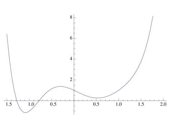
Figure 6. The graph of $t^{3}\cdot\Delta_{P(5,-3,8)}(t)$.

Clearly visible on the graph, the two real roots $t_{1,2}$ of $\Delta_{K}(t)$ are not of unit norm. The 4 complex roots are approximately

$$t_{3,4}=0.528853\pm 0.269329\,i\quad\quad\mbox{ and }\quad\quad t_{5,6}=1.50147\pm 0.764653\,i$$

showing that the approximate norms of $t_{3,4}$ and $t_{5,6}$ are

$$|t_{3,4}|=0.352223\quad\quad\mbox{ and }\quad\quad|t_{5,6}|=2.83911$$

Thus $\Delta_{K}(t)$ has no roots on $S^{1}$ so that $\sigma_{\omega}(K)=\sigma(K)$ for all $\omega\in S^{1}$. But $\sigma(K)=0$ as is easily computed from theorem 1.17. This implies that $K$ is of finite algebraic concordance order, cf. [7].

On the other hand, if $K$ were algebraically slice, then we could factor $\Delta_{K}(t)$ as $f(t)\cdot f(t^{-1})$ for some $f(t)\in\mathbb{Z}[t]$. This however is not the case. An easy way to see this is to note that the mod 2 reduction of $\Delta_{K}(t)$ looks like

$$\Delta_{K}(t) \equiv t^{3}+t+1+t^{-1}+t^{-3}(\mbox{ mod }2)$$

(110) $$\equiv(t+1+t^{-1})(t^{2}+t+1+t^{-1}+t^{-2})(\mbox{ mod }2)$$

Now, $t+1+t^{-1}$ is irreducible in $\mathbb{Z}_{2}[t,t^{-1}]$ but $t^{2}+t+1+t^{-1}+t^{-2}$ is not divisible by $t+1+t^{-1}$. Thus $\Delta_{K}(t)$ could not have factored as $f(t)\cdot f(t^{-1})$ and so $K$ is not algebraically slice. In fact, using Mathematica one finds that $\Delta_{K}(t)$ is irreducible over $\mathbb{Z}[t,t^{-1}]$.

Finally, the fact that $\varphi(K)=0\in W(\mathbb{Q})$ follows readily from theorem 1.11 since $\det K=1$, $5+(-3)=2$ and, as already mentioned, $\sigma(K)=0$. ∎

References

- [1] J. Greene and S. Jabuka, The slice-ribbon conjecture for 3-standed pretzel knots, Preprint (2007), ArXiv:0706.3398v2.
- [2] D. Husemoller and J. Milnor, Symmetric bilinear forms, Ergebnisse der Mathematik und ihrer Grenzgebiete 73, Springer-Verlag, New York, 1973.
- [3] M. A. Kervaire, Les nœuds de dimensions supérieures, Bull. Soc. Math. France 93 (1965), 225 – 271.
- [4] T. Y. Lam, Introduction to quadratic forms over fields, Graduate Studies in Math. 67, American Mathematical Society, Providence, RI, 2005.
- [5] J. Levine, Knot cobordism groups in codimension 2, Comment. Math. Helv. 44 (1969) 229–244.
- [6] J. Levine, Invariants of knot cobordism, Invent. Math. 8 (1969) 98–110.
- [7] C. Livingston, The algebraic concordance order of a knot, Preprint 2008, arXiv:0806.3068.
- [8] C. Livingston and S. Naik Obstructing four-torsion in the classical knot concordance group, J. Differential Geom. 51 (1999) 1–12.
- [9] A. Pfister, Zur Darstellung von als Summe von Quadraten in einem Körper, J. London Math. Soc. 40 (1965) 159–165.
- [10] A. Pfister, Quadratische Formen in beliebigen Körpern, Invent. Math. 1 (1966) 116–132.
- [11] D. Rolfsen, Knots and links, Mathematics Lecture Series 7, Publish or Perish Inc., Berkeley, CA, 1976, ix+439pp.
- [12] O. T. O’Meara, Introduction to quadratic forms, Classics in Mathematics, Springer-Verlag, New York, 2000.
- [13] E. Witt, Theorie der quadratischen Formen in beliebigen Körpern, J. Reine Angew. Math. 176 (1937), 31 – 44.