Analysis of Verification-based Decoding on the $q$-ary Symmetric Channel for Large $q$

Abstract

A new verification-based message-passing decoder for low-density parity-check (LDPC) codes is introduced and analyzed for the $q$-ary symmetric channel ($q$-SC). Rather than passing messages consisting of symbol probabilities, this decoder passes lists of possible symbols and marks some lists as verified. The density evolution (DE) equations for this decoder are derived and used to compute decoding thresholds. If the maximum list size is unbounded, then one finds that any capacity-achieving LDPC code for the binary erasure channel can be used to achieve capacity on the $q$-SC for large $q$. The decoding thresholds are also computed via DE for the case where each list is truncated to satisfy a maximum list-size constraint. Simulation results are also presented to confirm the DE results. During the simulations, we observed differences between two verification-based decoding algorithms, introduced by Luby and Mitzenmacher, that were implicitly assumed to be identical. In this paper, the node-based algorithms are evaluated via analysis and simulation.

The probability of false verification (FV) is also considered and techniques are discussed to mitigate the FV. Optimization of the degree distribution is also used to improve the threshold for a fixed maximum list size. Finally, the proposed algorithm is compared with a variety of other algorithms using both density evolution thresholds and simulation results.

I Introduction

Low-density parity-check (LDPC) codes are linear codes that were introduced by Gallager in 1962 [1] and re-discovered by MacKay in 1995 [2]. The ensemble of LDPC codes that we consider (e.g. see [3] and [4]) is defined by the edge degree distribution (d.d.) functions $\lambda(x)=\sum_{k\geq 2}\lambda_{k}x^{k-1}$ and $\rho(x)=\sum_{k\geq 2}\rho_{k}x^{k-1}$. The standard encoding and decoding algorithms are based on the bit-level operations. However, when applied to the transmission of data packets, it is natural to perform the encoding and decoding algorithm at the packet level rather than the bit level. For example, if we are going to transmit 32 bits as a packet, then we can use error-correcting codes over the, rather large, alphabet with $2^{32}$ elements.

Let the r.v.s $X$ and $Y$ be the input and output, respectively, of a $q$-ary symmetric channel ($q$-SC) whose transition probabilities are

$$\Pr(Y=y|X=x)=\left\{\begin{array}[]{lcl}1-p&\mbox{if $x=y$}\\ p/(q-1)&\mbox{if $x\neq y$,}\end{array}\right.$$

where $x,y\in GF(q)$. The capacity of the $q$-SC, $1+(1-p)\log_{q}(1-p)+p\log_{q}p-p\log_{q}(q-1)$, is approximately equal to $1-p$ symbols per channel use for large $q$. This implies the number of symbols which can be reliably transmitted per channel use of the $q$-SC with large $q$ is approximately equal to that of the BEC with erasure probability $p$. Moreover, the behavior of the $q$-SC with large $q$ is similar to the BEC in the sense that: i) incorrectly received symbols from the $q$-SC provide almost no information about the transmitted symbol and ii) error detection (e.g., a CRC) can be added to each symbol with negligible overhead [5].

Binary LDPC codes for the $q$-SC with moderate $q$ are proposed and optimized based on EXIT charts in [6] and [7]. It is known that the complexity of the FFT-based belief-propagation algorithm, for $q$-ary LDPC codes, scales like $O(q\log q)$. Even for moderate sizes of $q$, such as $q=256$, this renders such algorithms impractical. However, when $q$ is large, an interesting effect can be used to facilitate decoding: if a symbol is received in error, then it is essentially a randomly chosen element of the alphabet and it is very unlikely that the parity-check equations involving this symbol are satisfied.

Based on this idea, Luby and Mitzenmacher develop an elegant algorithm for decoding LDPC codes on the $q$-SC for large $q$ [8]. However, their paper did not present simulation results and left capacity-achieving ensembles as an interesting open problem. Metzner presented similar ideas earlier in [9] and [10], but the focus and analysis is quite different. Davey and MacKay also develop and analyze a symbol-level message-passing decoder over small finite fields in [11]. A number of approaches to the $q$-SC (for large $q$) based on interleaved Reed-Solomon codes are also possible [5] [12]. In [13], Shokrollahi and Wang discuss two ways of approaching capacity. The first uses a two-stage approach where the first stage uses a Tornado code and verification decoding. The second is, in fact, equivalent to one of the decoders we discuss in this paper. When we discovered this, the authors were kind enough to send us an extended abstract [14] which contains more details. Still, the authors did not consider the theoretical performance with a maximum list-size constraint, the actual performance of the decoder via simulation, or false verification (FV) due to cycles in the decoding graph. In this paper, we describe the algorithm in detail and consider those details.

Inspired by [8], we introduce list-message-passing (LMP) decoding with verification for LDPC codes on the $q$-SC. Instead of passing a single value between symbol and check nodes, we pass a list of candidates to improve the decoding threshold. This modification also increases the probability of FV. So, we analyze the causes of FV and discuss techniques to mitigate FV. It is worth noting that the LMP decoder we consider is somewhat different than the list extension suggested in [8]. Their approach uses a peeling-style decoder based on verification rather than erasures. Also, the algorithms in [8] are proposed in a node-based (NB) style but analyzed using message-based (MB) decoders. It is implicitly assumed that the two approaches are equivalent. In fact, this is not always true. In this paper, we consider the differences between NB and MB decoders and derive an asymptotic analysis for NB decoders.

The paper is organized as follows. In Section II, we describe the LMP algorithm and use density evolution (DE) [15] to analyze its performance. The difference between NB and MB decoders for the first (LM1) and second algorithm (LM2) in [8] is discussed and the NB decoder analysis is derived in Section III, respectively. The error floor of the LMP algorithms is considered in Section IV. In Section V, differential evolution is used to optimize code ensembles and simulation results are compared with the theoretical thresholds. The results are also compared with previously published results from [8] and [13]. In Section VI, simulation results are presented. Applications of the LMP algorithm are discussed and conclusions are given in Section VII.

II Description and Analysis

II-A Description of the Decoding Algorithm

The LMP decoder we discuss is designed mainly for the $q$-SC and is based on local decoding operations applied to lists of messages containing probable codeword symbols. The list messages passed in the graph have three types: verified (V), unverified (U) and erasure (E). Every V-message has a symbol value associated with it. Every U-message has a list of symbols associated with it. Following [8], we mark messages as verified when they are very likely to be correct. In particular, we will find that the probability of FV approaches zero as $q$ goes to infinity.

The LMP decoder works by passing list-messages around the decoding graph. Instead of passing a single code symbol (e.g., Gallager A/B algorithm [1]) or a probability distribution over all possible code symbols (e.g., [11]), we pass a list of values that are more likely to be correct than the other messages. At a check node, the output list contains all symbols which could satisfy the check constraint for the given input lists. At the check node, the output message will be verified if and only if all the incoming messages are verified. At a node of degree $d$, the associativity and commutativity of the node-processing operation allow it to be decomposed into $(d-1)$ basic operations (e.g., $a\!+\!b\!+\!c\!+\!d\!=\!(a\!+\!b)\!+\!(c\!+\!d)$). In such a scheme, the computational complexity of each basic operation is proportional to $s^{2}$ at the check node and $s\ln s$ at the variable node, where $s$ is the list size of the input list. The list size grows rapidly as the number of iterations increases. In order to make the algorithm practical, we have to truncate the list to keep the list size within some maximum value, denoted $S_{max}$. In our analysis, we also find that, after the number of iterations exceeds half the girth of the decoding graph, the probability of FV increases very rapidly. We analyze the reasons of FV and classify the FV’s into two types. We find that the codes described in [8] and [13] both suffer from type-II FV. In Section IV, we analyze these FV’s and propose a scheme that reduces the probability of FV.

The message-passing decoding algorithm using list messages (or LMP) applies the following simple rules to calculate the output messages for a check node:

• If all the input messages are verified, then the output becomes verified with the value which makes all the incoming messages sum to zero.

• If any input message is an erasure, then the output message becomes an erasure.

• If there is no erasure on the input lists, then the output list contains all symbols which could satisfy the check constraint for the given input lists.

• If the output list size is larger than $S_{max}$, then the output message is an erasure.

It applies the following rules to calculate the output messages of a variable node:

• If all the input messages are erasures or there are multiple verified messages which disagree, then output message is the channel received value.

• If any of the input messages are verified (and there is no disagreement) or a symbol appears more than once, then the output message becomes verified with the same value as the verified input message or the symbol which appears more than once.

• If there is no verified message on the input lists and no symbol appears more than once, then the output list is the union of all input lists.

• If the output message has list size larger than $S_{max}$, then the output message is the received value from the channel.

II-B DE for Unbounded List Size Decoding Algorithm

To apply DE to the LMP decoder with unbounded list sizes, denoted LMP-$\infty$ (i.e., $S_{max}=\infty$), we consider three quantities which evolve with the iteration number $i$. Let $x_{i}$ be the probability that the correct symbol is not on the list passed from a variable node to a check node. Let $y_{i}$ be the probability that the message passed from a variable node to a check node is not verified. Let $z_{i}$ be the average list size passed from a variable node to a check node. The same variables are “marked” $(\tilde{x}_{i},\tilde{y}_{i},\tilde{z}_{i})$ to represent the same values for messages passed from the check nodes to the variable nodes (i.e., the half-iteration value). We also assume all the messages are independent, that is, we assume that the bipartite graph has girth greater than twice the number of decoding iterations.

First, we consider the probability, $x_{i}$, that the correct symbol is not on the list. For any degree-$d$ check node, the correct message symbol will only be on the edge output list if all of the other $d-1$ input lists contain their corresponding correct symbols. This implies that $\tilde{x}_{i}=1-\rho(1-x_{i}$). For any degree-$d$ variable node, the correct message symbol is not on the edge output list only if it is not on any of the other $d-1$ edge input lists. This implies that $x_{i+1}=p\lambda(\tilde{x}_{i})$. This behavior is very similar to erasure decoding of LDPC codes on the BEC and gives the identical update equation

$$x_{i+1}=p\lambda\left(1-\rho(1-x_{i})\right)$$ (1)

where $p$ is the $q$-SC error probability. Note that throughout the DE analysis, we assume that $q$ is sufficiently large. Next, we consider the probability, $y_{i}$, that the message is not verified. For any degree-$d$ check node, an edge output message is verified only if all of the other $d-1$ edge input messages are verified. For any degree-$d$ variable node, an edge output message is verified if any symbol on the other $d-1$ edge input lists is verified or occurs twice which implies $\tilde{y}_{i}=1-\rho(1-y_{i})$. The event that the output message is not verified can be broken into the union of two disjoint events: (i) the correct symbol is not on any of the input lists, and (ii) the symbol from the channel is incorrect and the correct symbol is on exactly one of the input lists and not verified. For a degree-$d$ variable node, this implies that

$$\Pr(\textrm{not verified})=\left(\tilde{x}_{i}\right)^{d-1}+p(d-1)\left(\tilde{y}_{i}-\tilde{x}_{i}\right)\left(\tilde{x}_{i}\right)^{d-2}.$$ (2)

Summing over the d.d. gives the update equation

$$y_{i+1}=\lambda\left(1-\rho(1-x_{i})\right)+\\ p\left(\rho(1-x_{i})-\rho(1-y_{i})\right)\lambda^{\prime}\left(1-\rho(1-x_{i})\right).$$ (3)

It is important to note that (1) and (3) were published first in [13, Thm. 2] (by mapping $x_{i}=p_{i}$ and $y_{i}=p_{i}+q_{i}$), but were derived independently by us.

Finally, we consider the average list-size $z_{i}$. For any degree-$d$ check node, the output list size is equal to the product of the sizes of the other $d-1$ input lists. Since the mean of the product of i.i.d. random variables is equal to the product of the means, this implies that $\tilde{z}_{i}=\rho(z_{i})$. For any degree-$d$ variable node, the output list size is equal to one plus the sum of the sizes of the other $d-1$ input lists if the output is not verified and one otherwise. Again, the mean of the sum of $d-1$ i.i.d. random variables is simply $d-1$ times the mean of the distribution, so the average output list size is given by

$$1+\left(\left(\tilde{x}_{i}\right)^{d-1}+p(d-1)\left(\tilde{y}_{i}-\tilde{x}_{i}\right)\left(\tilde{x}_{i}\right)^{d-2}\right)(d-1)\tilde{z}_{i}.$$

This gives the update equation

$$z_{i+1}= 1\!+\!\left[\tilde{x}_{i}\lambda^{\prime}\left(\tilde{x}_{i}\right)\!+\!p\left(\tilde{y}_{i}\!-\!\tilde{x}_{i}\right)\left(\lambda^{\prime}\left(\tilde{x}_{i}\right)\!+\!\tilde{x}_{i}\lambda^{\prime\prime}\left(\tilde{x}_{i}\right)\right)\right]\rho(z_{i}).$$

For the LMP decoding algorithm, the threshold of an ensemble $(\lambda(x),\rho(x))$ is defined to be

$$p^{*}\triangleq\sup\left\{p\in(0,1]\bigg{|}p\lambda(1-\rho(1-x))<x\;\forall\;x\in(0,1]\right\}.$$

Next, we show that some codes can achieve channel capacity using this decoding algorithm.

Theorem II.1

Let $p^{*}$ be the threshold of the d.d. pair $(\lambda(x),\rho(x))$ and assume that the channel error rate $p$ is less than $p^{*}$. In this case, the probability $y_{i}$ that a message is not verified in the $i$-th decoding iteration satisfies $\lim_{i\rightarrow\infty}y_{i}\rightarrow 0$. Moreover, for any $\epsilon>0$, there exists a $q<\infty$ such that LMP decoding of a long random $(\lambda,\rho)$ LDPC code, on a $q$-SC with error probability $p$, results in a symbol error rate less than $\epsilon$.

Proof:

See Appendix A. ∎

Remark II.2

Note that the convergence condition, $p^{*}\lambda(1-\rho(1-x))<x$ for $x\in(0,1]$, is identical to the BEC case but that $x$ has a different meaning. In the DE equation for the $q$-SC, $x$ is the probability that the correct value is not on the list. In the DE equation for the BEC, $x$ is the probability that the message is an erasure. This tells us any capacity-achieving ensemble for the BEC is capacity-achieving for the $q$-SC with LMP-$\infty$ algorithm and large enough $q$. This also gives some intuition about the behavior of the $q$-SC for large $q$. For example, when $q$ is large, an incorrectly received value behaves like an erasure [5].

Corollary II.3

The code with d.d. pair $\lambda(x)=x$ and $\rho(x)=(1-\epsilon)x+\epsilon x^{2}$ has a threshold of $1-\frac{\epsilon}{1+\epsilon}$ and a rate of $r>\frac{\epsilon}{3(1+\epsilon)}$. Therefore, it achieves a rate of $\Theta(\delta)$ for a channel error rate of $p=1-\delta$.

Proof:

Follows from $\big{(}1-\frac{\epsilon}{1+\epsilon}\big{)}\lambda\left(1-\rho(1-x)\right)<x$ for $x\in(0,1]$ and Theorem II.1. ∎

Remark II.4

We believe that Corollary II.3 provides the first linear-time decodable construction of rate $\Theta(\delta)$ for a random-error model with error probability $1-\delta$. A discussion of linear-time encodable/decodable codes, for both random and adversarial errors, can be found in [16]. The complexity also depends on the required list size which may be extremely large (though independent of the block length). Unfortunately, we do not have explicit bounds on the alphabet size or list size required for this construction.

In practice, one cannot implement a list decoder with unbounded list size. Therefore, we also evaluate the LMP decoder under a bounded list-size assumption.

II-C DE for the Decoding Algorithm with Bounded List Size

First, we introduce some definitions and notation for the DE analysis with bounded list-size decoding algorithm. Note that, in the bounded list-size LMP algorithm, each list may contain at most $S_{max}$ symbols. For convenience, we classify the messages into four types:

(V)

Verified: message is verified and has list-size 1.

(E)

Erasure: message is an erasure and has list-size 0.

(L)

Correct on list: message is not verified or erased and the correct symbol is on the list.

(N)

Correct not on list: message is not verified or erased, and the correct symbol is not on the list.

For the first two message types, we only need to track the fractions, $V_{i}$ and $E_{i}$, of message types in the $i$-th iteration. For the third and the fourth types of messages, we also need to track the list sizes. Therefore, we track the generating function of the list size for these messages, given by $L_{i}(x)$ and $N_{i}(x)$. The coefficient of $x^{j}$ represents the probability that the message has list-size $j$. Specifically, $L_{i}(x)$ is defined by

$$L_{i}(x)=\sum_{j=1}^{S_{max}}l_{i,j}x^{j},$$

where $l_{i,j}$ is the probability that, in the $i$-th decoding iteration, the correct symbol is on the list and the message list has size $j$. The function $N_{i}(x)$ is defined similarly. This implies that $L_{i}(1)$ is the probability that the list contains the correct symbol and that it is not verified. For the same reason, $N_{i}(1)$ gives the probability that the list does not contain the correct symbol and that it is not verified. For the simplicity of expression, we denote the overall density as $P_{i}=[V_{i},E_{i},L_{i}(x),N_{i}(x)]$. The same variables are “marked” $(\tilde{V},\tilde{E},\tilde{L},\tilde{N}$ and $\tilde{P})$ to represent the same values for messages passed from the check nodes to the variable nodes (i.e., the half-iteration value).

Using these definitions, we find that DE can be computed efficiently using polynomial arithmetic. For convenience of analysis and implementation, we use a sequence of basic operations plus a separate truncation operator to represent a multiple-input multiple-output operation. We use $\boxplus$ to denote the check-node operator and $\otimes$ to denote the variable-node operator. Using this, the DE for the variable-node basic operation $P^{(3)}=\tilde{P}^{(1)}\otimes\tilde{P}^{(2)}$ is given by

$$V^{(3)}= \,\tilde{V}^{(1)}+\tilde{V}^{(2)}-\tilde{V}^{(1)}\tilde{V}^{(2)}+\tilde{L}^{(1)}(1)\tilde{L}^{(2)}(1)$$ (4)

$$E^{(3)}= \,\tilde{E}^{(1)}\tilde{E}^{(2)}$$ (5)

$$L^{(3)}(x)= \,\tilde{L}^{(1)}(x)\left(\tilde{E}^{(2)}+\tilde{N}^{(2)}(x)\right)$$

$$+\tilde{L}^{(2)}(x)\left(\tilde{E}^{(1)}+\tilde{N}^{(1)}(x)\right)$$ (6)

$$N^{(3)}(x)= \,\tilde{N}^{(1)}(x)\tilde{E}^{(2)}+\tilde{N}^{(2)}(x)\tilde{E}^{(1)}$$

$$+\tilde{N}^{(1)}(x)\tilde{N}^{(2)}(x).$$ (7)

Note that (4)-(7) do not yet consider the list-size truncation and the channel value. For the basic check-node operation $\tilde{P}^{(3)}=P^{(1)}\boxplus P^{(2)}$, the DE is given by

$$\tilde{V}^{(3)}= \,V^{(1)}V^{(2)}$$ (8)

$$\tilde{E}^{(3)}= \,E^{(1)}+E^{(2)}-E^{(1)}E^{(2)}$$ (9)

$$\tilde{L}^{(3)}(z)= \,\left[V^{(1)}L^{(2)}(z)+V^{(2)}L^{(1)}(z)\right.$$

$$\,\left.+\,L^{(1)}(x)L^{(2)}(y)\right]_{x^{j}y^{k}\rightarrow z^{jk}}$$ (10)

$$\tilde{N}^{(3)}(z)= \,\left[N^{(1)}(x)N^{(2)}(y)+N^{(1)}(x)\left(V^{(2)}y+L^{(2)}(y)\right)\right.$$

$$\,\left.+\,N^{(2)}(x)\left(V^{(1)}y+L^{(1)}(y)\right)\right]_{x^{j}y^{k}\rightarrow z^{jk}}$$ (11)

where the subscript $x^{j}y^{k}\rightarrow z^{jk}$ denotes the substitution of variables. Finally, the truncation of lists to size $S_{max}$ is handled by truncation operators which map densities to densities. We use $\mathcal{T}$ and $\mathcal{T^{\prime}}$ to denote the truncation operation at the check and variable nodes. Specifically, we truncate terms with degree higher than $S_{max}$ in the polynomials $L(x)$ and $N(x)$. At check nodes, the truncated probability mass is moved to $E$.

At variable nodes, lists longer than $S_{max}$ entries are replaced by the channel value. Let $P^{\prime}_{i}=\big{(}\tilde{P}_{i}^{\otimes k-1}\big{)}$ be the intermediate density which is the result of applying the basic operation $k-1$ times on $\tilde{P}_{i}$. After considering the channel value and list truncation, the symbol node message density is given by $\mathcal{T^{\prime}}(P^{\prime}_{i})$. To analyze this, we separate $L^{\prime}_{i}(x)$ into two terms: ${A^{\prime}_{i}}(x)$ with degree less than $S_{max}$ and $x^{S_{max}}{B^{\prime}_{i}}(x)$ with degree at least $S_{max}$. Likewise, we separate ${N^{\prime}_{i}}(x)$ into ${C^{\prime}_{i}}(x)$ and $x^{S_{max}}{D^{\prime}_{i}}(x)$. The inclusion of the channel symbol and the truncation are combined into a single operation

$${\textstyle P_{i}\!=\!\mathcal{T}^{\prime}\!\left(\left[{V^{\prime}_{i}},{E^{\prime}_{i}},{A^{\prime}_{i}}(x)\!+\!x^{S_{max}}{B^{\prime}_{i}}(x),{C^{\prime}_{i}}(x)\!+\!x^{S_{max}}{D^{\prime}_{i}}(x)\right]\right)}$$

defined by

$$V_{i}= \,{V^{\prime}_{i}}\!+\!(1-p)\left({A^{\prime}_{i}}(1)+{B^{\prime}_{i}}(1)\right)$$ (12)

$$E_{i}= \,0$$ (13)

$$L_{i}(x)= \,(1-p)x\left({E^{\prime}_{i}}\!+\!{C^{\prime}_{i}}(x)\!+\!{D^{\prime}_{i}}(1)\right)\!+\!px{A^{\prime}_{i}}(x)$$ (14)

$$N_{i}(x)= \,px\left({E^{\prime}_{i}}\!+\!{B^{\prime}_{i}}(1)\!+\!{C^{\prime}_{i}}(x)\!+\!{D^{\prime}_{i}}(1)\right).$$ (15)

Note that in (12), the term $(1-p)\left({A^{\prime}_{i}}(1)+{B^{\prime}_{i}}(1)\right)$ is due to the fact that messages are compared for possible verification before truncation.

The overall DE recursion is easily written in terms of the forward (symbol to check) density $P_{i}$ and the backward (check to symbol) density $\tilde{P}_{i}$ by taking the irregularity into account. The initial density is $P_{0}=[0,0,(1-p)x,px]$, where $p$ is the error probability of the $q$-SC channel, and the recursion is given by

$$\tilde{P}_{i}= \sum_{k=2}^{d_{c}}\rho_{k}\,\mathcal{T}\left(P_{i}^{\boxplus k-1}\right)$$ (16)

$$P_{i+1}= \sum_{k=2}^{d_{v}}\lambda_{k}\,\mathcal{T^{\prime}}\left(\tilde{P}_{i}^{\otimes k-1}\right).$$ (17)

Note that the DE recursion is not one-dimensional. This makes it difficult to optimize the ensemble analytically. It remains an open problem to find the closed-form expression of the threshold in terms of the maximum list size, d.d. pairs, and the alphabet size $q$. In section V, we will fix the maximum variable and check degrees, code rate, $q$ and maximum list size and optimize the threshold over the d.d. pairs by using a numerical approach.

III Analysis of Node-based Algorithms

III-A Differential Equation Analysis of LM1-NB

We refer to the first and second algorithms in [8] as LM1 and LM2, respectively. Each algorithm can be viewed either as message-based (MB) or node-based (NB). The first and second algorithms in [13] and [14] are referred to as SW1 and SW2. These algorithms are summarized in Table I. Note that, if no verification occurs, the variable node (VN) sends the (“channel value”, U) and the check node (CN) sends the (“expected correct value”,U) in all these algorithms. The algorithms SW1, SW2 and LMP are all MB algorithms, but can be modified to be NB algorithms.

III-A1 Motivation

TABLE I: Brief Description of Message-Passing Algorithms for $q$-SC

Alg.	Description
LMP-$S_{max}$	LMP as described in Section II-A with maximum
	list-size $S_{max}$
LM1-MB	MP decoder that passes (value, $U$/$V$). [8, III.B]
	At VN’s, output is $V$ if any input is $V$ or message
	matches channel value, otherwise pass channel value.
	At CN’s, output is $V$ iff all inputs are $V$.
LM1-NB	Peeling decoder with VN state (value, $U$/$V$). [8, III.B]
	At CN’s, if all neighbors sum to 0, all neighbors get $V$.
	At CN’s, if all neighbors but one are $V$, then last is $V$.
LM2-MB	The same as LM1-MB with one extra rule. [8, IV.A].
	At VN’s, if two input messages match, then output $V$.
LM2-NB	The same as LM1-NB with one extra rule. [8, IV.A].
	At VN’s, if two neighbor values same, then VN gets $V$.
SW1	Identical to LM2-MB
SW2	Identical to LMP-$\infty$. [13, Thm. 2]

In [8], the algorithms are proposed in the node-based (NB) style [8, Section III-A and IV], but analyzed in the message-based (MB) style [8, Section III-B and IV]. It is easy to verify that the LM1-NB and LM1-MB have identical performance, but this is not true for the NB and MB LM2 algorithms. In this section, we will show the differences between the NB decoder and MB decoder and derive a precise analysis for LM1-NB.

First, we discuss the equivalence of LM1-MB and LM1-NB.

Theorem III.1

Let $A$ be the set of variable nodes that are verified when LM1-NB decoding terminates. For the same received sequence, let $B$ be the set of variable nodes that have at least one verified output message when LM1-MB terminates. Then, LM1-NB and LM1-MB are equivalent in the sense that $A=B$.

Proof:

Though the basic idea behind this result is relatively straightforward, the details are somewhat lengthy and, therefore, deferred to a more general treatment [17]. The first observation is that the LM1-NB and LM1-MB decoders both satisfy a monotonicity property that, assuming no FV, guarantees convergence to a fixed point. In particular, the messages are ordered with respect to type (e.g., verified $>$ correct $>$ incorrect) and vectors of messages are endowed with the induced partial ordering. Using this approach, it can be shown that the fixed point messages of the LM1-NB decoder cannot be worse than those of the LM1-MB decoder. Finally, a detailed analysis of the computation tree, for an arbitrary LM1-MB fixed point, shows that every node verified by LM1-NB must have at least one verified output message. ∎

In the NB decoder, the verification status is associated with a node. Once a node is verified, all outgoing messages are verified. In the MB decoder, the status is associated with an edge and the outgoing message on each edge may have a different verification status. NB algorithms cannot, in general, be analyzed using DE because the independence assumption between messages does not hold. Therefore, we develop peeling-style decoders, which are equivalent to LM1-NB and LM2-NB, and use differential equations to analyze them.

It is worth noting that the threshold of a node-based algorithm is at least as large as its message-based counterpart. This is because node-based processing can only result in additional verifications during each step. The intuition behind this can be seen by looking at a variable node of degree 3. The message-based decoder may sometimes output a verified message on only one edge. This occurs, for example, if the channel value is incorrect and the three input messages are $V,I,I$. But, the node-based decoder verifies all output edges in this case. The drawback is that the correlation caused by node-based processing complicates the analysis because density evolution is based on the assumption that all input messages are independent.

Following [3], we analyze the peeling-style decoder using differential equations that track the average number of edges (grouped into types) in the graph as decoding progresses. From the results of [3] and [18], we know that the actual number of edges (of any type), in any particular decoding realization is tightly concentrated around the average over the lifetime of the random process. For peeling-style decoding, a variable node and its edges are removed after verification; each check node keeps track of its new parity constraint (i.e., the value to which the attached variables must sum) by subtracting values associated with the removed edges.

III-A2 Analysis of Peeling-Style Decoding

First, we introduce some notation and definitions for the analysis. A variable node (VN) whose channel value is correctly received is called a correct variable node (CVN), otherwise it is called an incorrect variable node (IVN). A check node (CN) with $i$ edges connected to the CVN’s and $j$ edges connected to the IVN’s will be said to have C-degree $i$ and I-degree $j$, or type $n_{i,j}$. We note that the analysis of node-based algorithms hold for irregular LDPC code ensemble of maximum variable node degree $d_{v}$ and maximum check node degree $d_{c}$.

We also define the following quantities:

• $t$: decoding time or fraction of VNs removed from graph

• $L_{i}(t)$: the number of edges connected to CVN’s with degree $i$ at time $t$

• $R_{j}(t)$: the number of edges connected to IVN’s with degree $j$ at time $t$

• $N_{i,j}(t)$: the number of edges connected to CN’s with C-degree $i$ and I-degree $j$

• $E_{l}(t)$: the remaining number of edges connected to CVN’s at time $t$

• $E_{r}(t)$: the remaining number of edges connected to IVN’s at time $t$

• $a(t)$: the average degree of CVN’s which have at least 1 edge coming from CN’s of type $n_{i,1},i\geq 1$,

  $$a(t)=\frac{\sum_{k=1}^{d_{v}}{kL_{k}(t)}}{E_{l}(t)}$$

• $b(t)$: the average degree of IVN’s which have at least 1 edge coming from CN’s of type $n_{0,1}$,

  $$b(t)=\frac{\sum_{k=1}^{d_{v}}{kR_{k}(t)}}{E_{r}(t)}$$

• $E$: number of edges in the original graph,

  $$E=E_{l}(0)+E_{r}(0).$$

Counting edges in three ways gives the identity

$$\sum_{i\geq 1}L_{i}(t)+\sum_{i\geq 1}R_{i}(t)=E_{l}(t)+E_{r}(t)=\!\!\!\!\sum_{\begin{subarray}{c}i\geq 0,j\geq 0\\ (i,j)\neq(0,0)\end{subarray}}\!\!\!\!N_{i,j}(t).$$

These r.v.’s represent a particular realization of the decoder. The differential equations are defined for the normalized (i.e., divided by $E$) expected values of these variables. We use lower-case notation (e.g., $l_{i}(t)$, $r_{i}(t)$, $n_{i,j}(t)$, etc.) for these deterministic trajectories. Time is scaled so that the decoder removes exactly one variable node during $1/N$ time units, where $N$ is the block length of the code.

The description of peeling-style decoder is as follows. The peeling-style decoder removes one CVN or IVN in each time step by the following rules:

CER:

If any CN has all its edges connected to CVN’s, remove one of these CVN’s and all of its edges.

IER1:

If any IVN has at least one edge connected to a CN of type $(0,1)$, then compute the value of the IVN from the attached CN and remove the IVN along with all its edges.

If both CER and IER1 can be applied, then one is chosen randomly as described below.

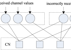
Figure 1: Tanner graph for the LM1 differential equation analysis.

Since both rules remove exactly one VN, the decoding process either finishes in exactly $N$ steps or stops early and cannot continue. The first case occurs only when either the IER1 or CER condition is satisfied in every time step. When the decoder stops early, the pattern of CVNs and IVNs remaining is called a stopping set. We also note that the rules above, though described differently, are equivalent to the first node-based algorithm (LM1-NB) introduced in [8].

Recall that the node-based algorithm for LM1, from [8], has two verification rules. The first rule is: if the neighbors (of a CN) have values that sum to zero, then all the neighbors are verified to their current values. In this analysis, however, the neighbors are verified one at a time. Since this implies that the CN is attached only to CVNs (assuming no FV), we call this correct-edge-removal (CER) and notice that it is only allowed if $n_{i,0}>0$ for some $i\geq 1$. The second rule is: if all neighbors (of a CN) are verified except for one, then the last neighbor is verified to the value that satisfies the check. If the last neighbor is an IVN, we call this type-I incorrect-edge-removal (IER1) and notice that it is only allowed when $n_{0,1}(t)>0$.

The peeling-style decoder performs one operation during each time step. The operation is random and can be either CER or IER1. When both operations are possible, we choose randomly between these two rules by picking CER with probability $c_{1}(t)$ and IER1 with probability $c_{2}(t)$, where

$$c_{1}(t) =\frac{\sum_{i\geq 1}n_{i,0}(t)}{\sum_{i\geq 1}n_{i,0}(t)+n_{0,1}(t)}$$

$$c_{2}(t) =\frac{n_{0,1}(t)}{\sum_{i\geq 1}n_{i,0}(t)+n_{0,1}(t)}.$$

This weighted sum ensures that the expected change in the decoder state is Lipschitz continuous if either $c_{1}(t)$ or $c_{2}(t)$ is strictly positive. Therefore, the differential equations can be written as

$$\frac{\mbox{d}l_{i}(t)}{\mbox{d}t} =c_{1}(t)\frac{\mbox{d}l_{i}^{(1)}(t)}{\mbox{d}t}+c_{2}(t)\frac{\mbox{d}l_{i}^{(2)}(t)}{\mbox{d}t}$$

$$\frac{\mbox{d}r_{i}(t)}{\mbox{d}t} =c_{1}(t)\frac{\mbox{d}r_{i}^{(1)}(t)}{\mbox{d}t}+c_{2}(t)\frac{\mbox{d}r_{i}^{(2)}(t)}{\mbox{d}t}$$

$$\frac{\mbox{d}n_{i,j}(t)}{\mbox{d}t} =c_{1}(t)\frac{\mbox{d}n_{i,j}^{(1)}(t)}{\mbox{d}t}+c_{2}(t)\frac{\mbox{d}n_{i,j}^{(2)}(t)}{\mbox{d}t},$$

where ⁽¹⁾ and ⁽²⁾ denote, respectively, the effects of CER and IER1.

III-A3 CER Analysis

If the CER operation is picked, then we choose randomly an edge attached to a CN of type $(i,0)$ with $i\geq 1$. This VN endpoint of this edge is distributed uniformly across the CVN edge sockets. Therefore, it will be attached to a CVN of degree $k$ with probability ${l_{k}(t)}/{e_{l}(t)}$. Therefore, one has the following differential equations for $l_{k}$ and $r_{k}$

$$\frac{\mbox{d}l_{k}^{(1)}(t)}{\mbox{d}t}=\frac{l_{k}(t)}{e_{l}(t)}(-k),\textrm{ for }k\geq 1$$

and

$$\frac{\mbox{d}r_{k}^{(1)}(t)}{\mbox{d}t}=0.$$

For the effect on check edges, we can think of removing a CVN with degree $k$ as first randomly picking an edge of type $(k,0)$ connected to that CVN and then removing all the other $k-1$ edges (called reflected edges) attached to the same CVN. The $k-1$ reflected edges are uniformly distributed over the $E_{l}(t)$ correct sockets of the CN’s. These $k-1$ reflected edges hit $\frac{n_{i,j}(t)i(k-1)}{(i+j)e_{l}(t)}$ CN’s of type $(i,j)$ on average. Next, we average over the VN degree, $k$, and find that

$$p_{i,j}^{(1)}(t)\triangleq\frac{n_{i,j}(t)i(a(t)-1)}{(i+j)e_{l}(t)}$$

is the expected number of type-$(i,j)$ CN’s hit by reflected edges.

If a CN of type $(i,j)$ is hit by a reflected edge, then the decoder state loses $i+j$ edges of type $(i,j)$ and gains $i-1+j$ edges of type $(i-1,j)$. Hence, one has the following differential equation, for $j>0$ and $i+j\leq d_{c}$,

$$\frac{\mbox{d}n_{i,j}^{(1)}(t)}{\mbox{d}t}=\left(p_{i+1,j}^{(1)}(t)-p_{i,j}^{(1)}(t)\right)(i+j).$$

One should keep in mind that $n_{i,j}(t)=0$ for $i+j>d_{c}$.

For $n_{i,j}^{(1)}(t)$ with $j=0$, the effect from above must be combined with effect of the type-$(i,0)$ initial edge that was chosen. So the differential equation becomes

$$\frac{\mbox{d}n_{i,0}^{(1)}(t)}{\mbox{d}t}=\left(p_{i+1,0}^{(1)}(t)-p_{i,0}^{(1)}(t)\right)i+\left(q_{i+1}^{(1)}(t)-q_{i}^{(1)}(t)\right)i$$

where

$$q_{i}^{(1)}(t)\triangleq\frac{n_{i,0}(t)}{\sum_{m\geq 1}n_{m,0}(t)}.$$

Note that $p^{(1)}_{d_{c}+1,0}(t)\triangleq 0$ and $q^{(1)}_{d_{c}+1}(t)\triangleq 0$

III-A4 IER1 Analysis

If the IER1 operation is picked, then we choose a random CN of type $(0,1)$ and follow its only edge to the set of IVNs. The edge is attached uniformly to this set, so the differential equations for IER1 are given by

$$\frac{\mbox{d}l_{k}^{(2)}(t)}{\mbox{d}t}=0,$$

$$\frac{\mbox{d}r_{k}^{(2)}(t)}{\mbox{d}t}=\frac{r_{k}(t)}{e_{r}(t)}(-k),$$

and

$$\frac{\mbox{d}n_{i,j}^{(2)}(t)}{\mbox{d}t}=\left(p_{i,j+1}^{(2)}(t)-p_{i,j}^{(2)}(t)\right)(i+j)-\delta_{i,0}\delta_{j,1},$$

where

$$p_{i,j}^{(2)}(t)\triangleq\frac{n_{i,j}(t)j(b(t)-1)}{(i+j)e_{r}(t)}.$$

We note that the removal of the initial edge, when $(i,j)=(0,1)$, is taken into account by the Kronecker delta functions.

Notice that even for (3,6) codes, there are 30 differential equations to solve. So we solve the differential equations numerically and the threshold for (3,6) code with LM1 is $p^{*}=0.169$. This coincides with the result from density evolution analysis for LM1-MB in [8] and hints at the equivalence between LM1-NB and LM1-MB. In the proof of Theorem III.1 we make this equivalence precise by showing that the stopping sets of LM1-NB and LM1-MB are the same.

III-B Differential Equation Analysis of LM2-NB

Similar to the analysis of LM1-NB algorithm, we analyze LM2-NB algorithm by analyzing a peeling-style decoder which is equivalent to the LM2-NB decoding algorithm. The peeling-style decoder removes one CVN or IVN during each time step according to the following rules:

CER:

If any CN has all its edges connected to CVN’s, pick one of the CVN’s and remove it.

IER1:

If any IVN has any messages from CN’s with type $n_{0,1}$, then the IVN and all its outgoing edges can be removed and we track the correct value by subtracting the value from the check node.

IER2:

If any IVN is attached to more than one CN with I-degree 1, then it will be verified and all its outgoing edges can be removed.

For simplicity, we first introduce some definitions and short-hand notation:

• Correct edges: edges which are connected to CVN’s

• Incorrect edges: edges which are connected to IVN’s

• CER edges: edges which are connected to check nodes with type $n_{i,0}$ for $i\geq 1$

• IER1 edges: edges which are connected to check nodes with type $n_{0,1}$

• IER2 edges: edges which connect IVN’s and the check nodes with type $n_{i,1}$ for $i\geq 1$

• NI edges: normal incorrect edges, which are incorrect edges but neither IER1 edges nor IER2 edges

• CER nodes: CVN’s which have at least one CER edge

• IER1 nodes: IVN’s which have at least one IER1 edge

• IER2 nodes: IVN’s which have at least two IER2 edges

• NI nodes: IVN’s which contain at most 1 IER2 edge and no IER1 edges.

Note that an IVN can be both an IER1 node and an IER2 node at the same time.

The analysis of LM2-NB is much more complicated than LM1-NB because the IER2 operation makes the distribution of IER2 edges dependent on each other. For example, the IER2 operation removes a randomly chosen IVN with more than 2 IER2 edges; this reduces the number of IVNs which have multiple IER2 edges and therefore the remaining IER2 edges are more likely to land on different IVN’s.

The basic idea behind our analysis of the LM2-NB decoder is that we can separate the incorrect edges into types and assume that mapping between sockets is given by a uniform random permutation. Strictly speaking, this is not true and another approach, which leads to the same differential equations, is used when considering a formal proof of correctness. In detail, we model the structure of an LDPC code during LM2-NB decoding as shown in Fig. 2 with one type for correct edges and three types for incorrect edges. The following calculations assume the four permutations, labeled CER, NI, IER2, and IER1, are all uniform random permutations.

Figure 2: Graph structure of an LDPC code during LM2-NB decoding.

The peeling-style decoder randomly chooses one VN from the set of CER IER1 and IER2 nodes and removes this node and all its edges at each step. The idea of the analysis is to first calculate the probability of choosing a VN with a certain type, i.e., CER, IER1 or IER2, and the node degree. We then analyze how removing this VN affects the system parameters.

In the analysis, we will track the evolution of the following system parameters:

• $l_{k}(t)$: the fraction of edges connected to CVN’s with degree $k$, $0<k\leq d_{v}$ at time $t$

• $r_{i,j,k}(t):$ the fraction of edges connected to IVN’s with $i$ NI edges, $j$ IER2 edges and $k$ IER1 edges at time $t$, $i,j,k\in\{0,1,\dots,d_{v}\}$ and $0<i+j+k\leq d_{v}$

• $n_{i,j}(t):$ the fraction of edges connected to check nodes with $i$ correct edges and $j$ incorrect edges at time $t$, $i,j\in\{0,1,\dots,d_{c}\}$ and $0<i+j\leq d_{c}$.

We note that, when we say “fraction”, we mean the number of a certain type of edges/nodes normalized by the number of edges/nodes in the original graph.

The following quantities can be calculated from $l_{k}(t)$, $r_{i,j,k}(t)$ and $n_{i,j}(t)$:

• $e_{l}(t)\triangleq\sum_{k=1}^{d_{v}}l_{k}(t)$: the fraction of correct edges

• $e_{r}(t)\triangleq\sum_{i=0}^{d_{v}}\sum_{j=0}^{d_{v}-i}\sum_{k=0}^{d_{v}-i-j}r_{i,j,k}(t)$: the fraction of incorrect edges

• $\eta_{0}(t)\triangleq\sum_{j=2}^{d_{c}}\sum_{i=0}^{d_{c}-j}\frac{jn_{i,j}(t)}{i+j}\\ =\sum_{i=1}^{d_{v}}\sum_{j=0}^{d_{v}-i}\sum_{k=0}^{d_{v}-i-j}\frac{ir_{i,j,k}(t)}{i+j+k}$: the fraction of NI edges

• $\eta_{1}(t)\triangleq n_{0,1}(t)=\sum_{k=1}^{d_{v}}\sum_{j=0}^{d_{v}-k}\sum_{i=0}^{d_{v}-i-j}\frac{kr_{i,j,k}(t)}{(i+j+k)}$: the fraction of IER1 edges

• $\eta_{2}(t)\triangleq\sum_{i=1}^{d_{c}}\frac{n_{i,1}(t)}{(i+1)}\\ =\sum_{j=1}^{d_{v}}\sum_{i=0}^{d_{v}-j}\sum_{k=0}^{d_{v}-i-j}\frac{jr_{i,j,k}(t)}{(i+j+k)}$: the fraction of IER2 edges

• $s_{0}(t)\triangleq\sum_{j=0}^{1}\sum_{i=1}^{d_{v}-j}\frac{r_{i,j,0}}{i+j}$: the fraction of NI nodes

• $s_{1}(t)\triangleq\sum_{k=1}^{d_{v}}\frac{n_{k,0}(t)}{k}$: the fraction of CER nodes

• $s_{2}(t)\triangleq\sum_{k=1}^{d_{v}}\sum_{i=0}^{d_{v}-k}\sum_{j=0}^{d_{v}-i-k}\frac{r_{i,j,k}}{i+j+k}$: the fraction of IER1 nodes

• $s_{3}(t)\triangleq\sum_{j=2}^{d_{v}}\sum_{i=0}^{d_{v}-j}\sum_{k=0}^{d_{v}-i-j}\frac{r_{i,j,k}}{i+j+k}$: the fraction of IER2 nodes.

As in the LM1-NB analysis, we use superscript ⁽¹⁾ to denote the contribution of the CER operations. We use ⁽²⁾ to denote the contribution of the IER1 operations and ⁽³⁾ to denote the contribution of the IER2 operations. Since we assume that the decoder randomly chooses a VN from the set of CER, IER1 and IER2 nodes and removes all its edges during each time step, the differential equations of the system parameters can be written as the weighted sum of the contributions of the CER, IER1 and IER2 operations. The weights are chosen to be

$$c_{1}(t) =\frac{s_{1}(t)}{(s_{1}(t)+s_{2}(t)+s_{3}(t))}$$

$$c_{2}(t) =\frac{s_{2}(t)}{(s_{1}(t)+s_{2}(t)+s_{3}(t))}$$

$$c_{3}(t) =\frac{s_{3}(t)}{(s_{1}(t)+s_{2}(t)+s_{3}(t))}.$$

This weighted sum ensures that the expected change in the decoder state is Lipschitz continuous if any one $c_{1}(t)$, $c_{2}(t)$, or $c_{3}(t)$ is strictly positive. Next, we will show how CER, IER1 and IER2 operations affect the system parameters.

Given the d.d. pair $(\lambda,\rho)$ and the channel error probability $p$, we initialize the state as follows. Since a fraction $(1-p)\lambda_{k}$ of the edges are connected to CVN’s of degree $k$, we initialize $l_{k}(t)$ with

$$l_{k}(0)=(1-p)\lambda_{k},$$

for $k=1,2,\dots d_{v}$. Noticing that each CN socket is connected to a correct edge with probability $(1-p)$ and incorrect edge with probability $p$, we initialize $n_{i,j}(t)$ with

$$n_{i,j}(0)=\rho_{i+j}\binom{i+j}{i}(1-p)^{i}p^{j},$$

for $i+j\in\{1,2,\dots,d_{c}\}$. The probability that an IVN socket is connected to an NI, IER1 edge, or IER2 edge is denoted respectively by $g_{0}$, $g_{1}$, or $g_{2}$ with

$$g_{0} =\frac{1}{p}\sum_{j^{\prime}=2}^{d_{c}}\sum_{i^{\prime}=0}^{d_{c}-j^{\prime}}\frac{j^{\prime}n_{i^{\prime},j^{\prime}}(0)}{i^{\prime}+j^{\prime}}$$

$$g_{1} =\frac{1}{p}\sum_{i^{\prime}=1}^{d_{c}}\frac{n_{i^{\prime},1}(0)}{(i^{\prime}+1)}$$

$$g_{2} =\frac{1}{p}n_{0,1}(0).$$

Therefore, we initialize $r_{i,j,k}(t)$ with

$$r_{i,j,k}(0)=p\lambda_{i+j+k}\binom{i+j+k}{i,j,k}g_{0}^{i}g_{1}^{j}g_{2}^{k},$$

for $i+j+k\in\{1,2,\dots,d_{v}\}$.

III-B1 CER analysis

The analysis for $\frac{\textrm{d}l_{k}^{(1)}(t)}{\textrm{d}t}$ is the same as the LM1-NB analysis. In the CER operation, the decoder randomly selects a CER edge. A CVN with degree $k$ is chosen with probability ${l_{k}(t)}/{e_{l}(t)}$. If a degree $k$ CVN is chosen, the number of edges of type $l_{k}$ decreases by $k$ and therefore

$$\frac{\mbox{d}l_{k}^{(1)}(t)}{\mbox{d}t}=\frac{-kl_{k}(t)}{e_{l}(t)}.$$

For $j\geq 1$ and $i+j\leq d_{c}$

$$\frac{\mbox{d}n_{i,j}^{(1)}(t)}{\mbox{d}t}=\left(p_{i+1,j}^{(1)}(t)-p_{i,j}^{(1)}(t)\right)(i+j)$$

where $a(t)=\frac{\sum_{k=1}^{d_{v}}kl_{k}(t)}{e_{l}(t)}$ is the average degree of the CVN’s which are hit by the initially chosen CER edge and $p_{i,j}^{(1)}=\frac{n_{i,j}(t)i(a(t)-1)}{(i+j)e_{l}(t)}$ is the average number of CN’s with type $n_{i,j}$ hit by the $a(t)-1$ reflecting edges.

For $j=0$ and $i\geq 1$, we also have to consider the initially chosen CER edge. This gives

$$\frac{\mbox{d}n_{i,0}^{(1)}(t)}{\mbox{d}t}=\left(p_{i+1,0}^{(1)}(t)-p_{i,0}^{(1)}(t)\right)i+\left(q_{i+1}^{(1)}(t)-q_{i}^{(1)}(t)\right)i$$

where $q_{i}^{(1)}(t)=\frac{n_{i,0}(t)}{\sum_{m\geq 1}n_{m,0}(t)}$ is the probability that the initially chosen CER edge is of type $n_{i,0}$.

When the removed CER node has a reflecting edge that hits a CN of type $n_{1,1}$, the CN’s IER2 edge becomes an IER1 edge. This is the only way the CER operation can affect $r_{i,j,k}.$ On average, each CER operation generates $a(t)-1$ reflecting edges. For each reflecting edge, the probability that it hits a CN of type $n_{1,1}$ is $\frac{n_{1,1}(t)}{2e_{l}(t)}$. Taking this IER2 to IER1 conversion into account, for $k\geq 1$ and $j<d_{v}$, gives

$$\frac{\textrm{d}r_{i,j,k}^{(1)}(t)}{\mbox{d}t}=\,(a(t)\!-\!1)\frac{n_{1,1}(t)}{2e_{l}(t)}\left(\frac{jr_{i,j,k}(t)}{(i\!+\!j\!+\!k)\eta_{2}(t)}(-(i\!+\!j\!+\!k))\right.$$

$$\quad\quad\quad\quad\quad\left.-\frac{(j+1)r_{i,j+1,k-1}(t)}{(i\!+\!j\!+\!k)\eta_{2}(t)}(-(i\!+\!j\!+\!k))\right)$$

$$\quad=(a(t)\!-\!1)\frac{n_{1,1}(t)}{2e_{l}(t)}\left(\frac{-jr_{i,j,k}(t)}{\eta_{2}(t)}+\frac{(j\!+\!1)r_{i,j+1,k-1}(t)}{\eta_{2}(t)}\right).$$

If $k=0$ or $j=d_{v}$, then the IVN’s with type $r_{i,j,k}$ can only lose edges and

$$\frac{\textrm{d}r_{i,j,k}^{(1)}(t)}{\textrm{d}t}=(a(t)-1)\frac{n_{1,1}(t)}{2e_{l}(t)}\left(\frac{-jr_{i,j,k}(t)}{\eta_{2}(t)}\right).$$

III-B2 IER2 analysis

Since the IER2 operation does not affect $l_{k}(t)$, we have

$$\frac{\mbox{d}l_{k}^{(3)}(t)}{\mbox{d}t}=0.$$

To analyze how the IER2 operation changes $n_{i,j}(t)$ and $r_{i,j,k}(t)$, we first observe that the probability a randomly chosen IER2 node is of type $r_{i,j,k}$ is given by

$$\Pr\left(\mbox{type }r_{i,j,k}\,|\,\mbox{IER2 node}\right)=\frac{\frac{r_{i,j,k}(t)}{i+j+k}}{s_{3}(t)},$$

for $j\geq 2$. Otherwise, $\Pr\left(\mbox{type }r_{i,j,k}\,|\,\mbox{IER2 node}\right)=0$.

Let us denote the contribution to $\frac{\textrm{d}n_{i^{\prime},j^{\prime}}^{(3)}(t)}{\textrm{d}t}$ caused by removing: one NI edge as $u_{i^{\prime},j^{\prime}}(t)$, one IER2 edge as $v_{i^{\prime},j^{\prime}}(t)$, and one IER1 edge as $w_{i^{\prime},j^{\prime}}(t)$. Then, we can write the total contribution to the derivative as

$$\frac{\textrm{d}n_{i^{\prime},j^{\prime}}^{(3)}(t)}{\textrm{d}t}=\sum_{i=0}^{d_{v}}\sum_{j=0}^{d_{v}}\sum_{k=0}^{d_{v}}\Pr\left(\mbox{type }r_{i,j,k}\,|\,\mbox{IER2 node}\right)\\ \left(iu_{i^{\prime},j^{\prime}}(t)+jv_{i^{\prime},j^{\prime}}(t)+kw_{i^{\prime},j^{\prime}}(t)\right).$$

First, we consider $u_{i^{\prime},j^{\prime}}(t)$. If an NI edge is chosen from the IVN side, then it hits a CN of type $n_{i,j}$ with probability $\frac{jn_{i,j}(t)}{\eta_{0}(i+j)}$ if $j\geq 2$ and probability 0 otherwise. When $2\leq j\leq d_{v}-1$, we have

$$u_{i^{\prime},j^{\prime}}(t) =\frac{j^{\prime}n_{i^{\prime},j^{\prime}}(t)(-(i^{\prime}+j^{\prime}))}{(i^{\prime}+j^{\prime})\eta_{0}(t)}+\frac{(j^{\prime}+1)n_{i^{\prime},j^{\prime}+1}(i^{\prime}+j^{\prime})}{(i^{\prime}+j^{\prime}+1)\eta_{0}(t)}$$

$$=\frac{-j^{\prime}n_{i^{\prime},j^{\prime}}(t)}{\eta_{0}(t)}+\frac{(j^{\prime}+1)n_{i^{\prime},j^{\prime}+1}(i^{\prime}+j^{\prime})}{(i^{\prime}+j^{\prime}+1)\eta_{0}(t)}.$$

When $j=d_{v}$, one finds instead that

$$u_{i^{\prime},j^{\prime}}(t)=\frac{-j^{\prime}n_{i^{\prime}j^{\prime}}(t)}{\eta_{0}(t)}.$$

Since an NI edge cannot be connected to a CN of type $n_{i^{\prime},1}$, we must treat $j^{\prime}=1$ separately. Notice that type $n_{i^{\prime},1}$ may still gain edges from type $n_{i^{\prime},2}$, so we have

$$u_{i^{\prime},1}(t)=\frac{2n_{i^{\prime},2}(t)(i^{\prime}+1)}{(i^{\prime}+2)\eta_{0}(t)}.$$

When $j^{\prime}=0$, CN’s with type $n_{i^{\prime},0}$ do not have any NI edges, so we have $u_{i^{\prime},0}(t)=0$. Now we consider $v_{i^{\prime},j^{\prime}}(t)$. Since edges of type $n_{i^{\prime},j^{\prime}}$ with $j\geq 2$ cannot be IER2 edges, $n_{i^{\prime}j^{\prime}}(t)$ with $j\geq 2$ is not affected by removing IER2 edges. The IER2 edge removal reduces the number of edges of type $n_{i^{\prime},1}$, $i\geq 1$, so we have $v_{i^{\prime},1}(t)=-\frac{n_{i^{\prime},1}(t)}{\eta_{2}(t)}$. When $j^{\prime}=0$ and $i^{\prime}\geq 1$, we have $v_{i^{\prime},0}(t)=\frac{n_{i^{\prime},1}(t)}{\eta_{2}(t)}$. Only CN’s with type $n_{0,1}$ are affected when we remove an IER1 edge on the IVN side. So we have $w_{0,1}(t)=1$ and $w_{i^{\prime},j^{\prime}}(t)=0$ when $(i^{\prime},j^{\prime})(t)\neq(0,1).$

Next, we derive the contribution to the $r_{i,j,k}(t)$ differential equation caused by removing an IER2 node. When the decoder removes an IER2 node of type $r_{i^{\prime},j^{\prime},k^{\prime}}$, there are direct and indirect effects. The direct effect is the loss of $i^{\prime}$ NI edges, $j^{\prime}$ IER2 edges and $k^{\prime}$ IER1 edges. This edge removal affects CN degrees and the type of some CN edges may also change and thereby indirectly affect $r_{i,j,k}(t)$. We call these indirectly affected edges “CN reflected edges”.

Let $u^{\prime}_{i,j,k}(t)$ be the contribution of CN reflected edges to $\frac{\textrm{d}r_{i,j,k}(t)}{\textrm{d}t}$ caused by the removal of: an NI edge be $u^{\prime}_{i,j,k}(t)$, an IER2 edge be $v^{\prime}_{i,j,k}(t)$, and an IER2 edge be $w^{\prime}_{i,j,k}(t)$. Then, we can write the total contribution to the derivative as

$$\frac{\textrm{d}r_{i,j,k}^{(3)}(t)}{\textrm{d}t}=-\Pr\left(\mbox{type }r_{i,j,k}\,|\,\mbox{IER2 node}\right)(i+j+k)\,+\\ \sum_{i^{\prime}=0}^{d_{v}}\sum_{j^{\prime}=0}^{d_{v}}\sum_{k^{\prime}=0}^{d_{v}}\Pr\left(\mbox{type }r_{i^{\prime},j^{\prime},k^{\prime}}\,|\,\mbox{IER2 node}\right)\\ \left(i^{\prime}u^{\prime}_{i,j,k}(t)+j^{\prime}v^{\prime}_{i,j,k}(t)+k^{\prime}w^{\prime}_{i,j,k}(t)\right).$$

There are two ways that the CN reflected edges of an NI edge can affect $r_{i,j,k}(t)$. The first occurs when the CN is of type $n_{i,2}$ and $1\leq i\leq d_{c}-2$. In this case, removing an NI edge changes the type of the other incorrect edge from NI to IER2. The second occurs when the CN is of type $n_{0,2}$. Removing an NI edge changes the type of the other incorrect edge from NI to IER1. The probability that an NI edge hits a CN of type $n_{i,2},$ (for $1\leq i\leq d_{c}-2$) is $\frac{\sum_{i=1}^{d_{c}-2}\frac{2n_{i,2}(t)}{i+2}}{\eta_{0}(t)}$. Likewise, the probability that an NI edge hits a CN of type $n_{0,2}$ is $\frac{n_{0,2}(t)}{\eta_{0}(t)}$. Since the probability that an NI edge is connected to an IVN of type $r_{i,j,k}$ is $\frac{ir_{i,j,k}(t)}{(i+j+k)\eta_{0}(t)}$, one finds that

$$u^{\prime}_{i,j,k}(t) \!=\!\frac{\sum_{i=1}^{d_{c}-2}\frac{2n_{i,2}(t)}{i+2}}{\eta_{0}(t)}\!\left(\!-\frac{ir_{i,j,k}(t)}{\eta_{0}(t)}\!+\!\frac{(i\!+\!1)r_{i+1,j-1,k}(t)}{\eta_{0}(t)}\right)$$

$$+\frac{n_{0,2}(t)}{\eta_{0}(t)}\left(-\frac{ir_{i,j,k}(t)}{\eta_{0}(t)}+\frac{(i+1)r_{i+1,j,k-1}(t)}{\eta_{0}(t)}\right),$$

where $r_{i,j,k}(t)\triangleq 0$ unless $i,j,k\in\{0,\ldots,d_{v}\}$ and $i+j+k\leq d_{v}$. Since there are no CN reflected edges of type IER1 and IER2, one also finds that $v^{\prime}_{i,j,k}(t)=0$ and $w^{\prime}_{i,j,k}(t)=0$.

III-B3 IER1 Analysis

Like the IER2 operation, the IER1 operation does not affect $l_{k}(t)$ and therefore

$$\frac{\textrm{d}l_{k}^{(2)}(t)}{\textrm{d}t}=0.$$

To analyze how IER1 changes $n_{i,j}(t)$ and $r_{i,j,k}(t)$, we observe that the probability a randomly chosen IER1 node is of type $r_{i,j,k}$ is given by

$$\Pr\left(\mbox{type }r_{i,j,k}\,|\,\mbox{IER1 node}\right)=\frac{\frac{r_{i,j,k}(t)}{i+j+k}}{s_{2}(t)}$$

when $k\geq 1$. Otherwise, $\Pr\left(\mbox{type }r_{i,j,k}\,|\,\mbox{IER1 node}\right)=0$.

Applying the same arguments used for the IER2 operation, one finds that,

$$\frac{\textrm{d}n_{i^{\prime},j^{\prime}}^{(2)}(t)}{\textrm{d}t}=\sum_{i=0}^{d_{v}}\sum_{j=0}^{d_{v}}\sum_{k=0}^{d_{v}}\Pr\left(\mbox{type }r_{i,j,k}\,|\,\mbox{IER1 node}\right)\\ \left(iu_{i^{\prime},j^{\prime}}(t)+jv_{i^{\prime},j^{\prime}}(t)+kw_{i^{\prime},j^{\prime}}(t)\right)$$

and

$$\frac{\textrm{d}r_{i,j,k}^{(2)}(t)}{\textrm{d}t}=-\Pr\left(\mbox{type }r_{i^{\prime},j^{\prime},k^{\prime}}\,|\,\mbox{IER1 node}\right)(i^{\prime}+j^{\prime}+k^{\prime})\\ +\sum_{i^{\prime}=0}^{d_{v}}\sum_{j^{\prime}=0}^{d_{v}}\sum_{k^{\prime}=0}^{d_{v}}\Pr\left(\mbox{type }r_{i^{\prime},j^{\prime},k^{\prime}}\,|\,\mbox{IER1 node}\right)\\ \left(i^{\prime}u^{\prime}_{i,j,k}(t)+j^{\prime}v^{\prime}_{i,j,k}(t)+k^{\prime}w^{\prime}_{i,j,k}(t)\right).$$

The program used to perform these computations and compute LM2-NB thresholds is available online [19].

III-C Discussion of the Analysis

Consider the peeling decoder for the BEC introduced in [8]. Throughout the decoding process, one reveals and then removes edges one at a time from a hidden random graph. The analysis of this decoder is simplified by the fact that, given the current residual degree distribution, the unrevealed portion of the graph remains uniform for every decoding trajectory. In fact, one can build a finite-length decoding simulation never constructs the actual decoding graph. Instead, it tracks only the residual degree distribution of the graph and implicitly chooses a random decoding graph one edge at a time.

For asymptotically long codes,[8] used this approach to derive an analysis based on differential equations. This analysis is actually quite general and can also be applied to other peeling-style decoders in which the unrevealed graph is not uniform. One may observe this from its proof of correctness, which depends only on two important observations. First, the distribution of all decoding paths is concentrated very tightly around its average as the system size increases. Second, the expected change in the decoder state can be written as a Lipschitz function of the current decoder state. If one augments the decoding state to include enough information so that the expected change can be computed from the augmented state (even for non-uniform residual graphs), then the theorem still applies.

The differential equation computes the average evolution, over all random bipartite graphs, of the system parameters as the block length $n$ goes to infinity. While the numerical simulation of long codes gives the evolution of the system parameters of a particular code (a particular bipartite graph) as $n$ goes to infinity. To prove that the differential equation analysis precisely predicts the evolution of the system parameters of a particular code, one must show the concentration of the evolution of the system parameters of a particular code around the ensemble average as $n$ goes to infinity.

In the LM2-NB algorithm, one node is removed at a time but this can also be viewed as removing each edge sequentially. The main difference for LM2-NB algorithm is that one has more edge types and one must track some details of the edge types on both the check nodes and the variable nodes. This causes a significant problem in the analysis because updating the exact effect of edge removal requires revealing some edges before they will be removed. For example, the CER operation can cause an IER2 edge to become an IER1 edge, but revealing the adjacent symbol node (or type) renders the analysis intractable.

Unfortunately, our proof of correctness still relies on two unproven assumptions which we state as a conjectures. This section leverages the framework of [8, 18, 20] by describing only the new discrete-time random process $H_{t}$ associated with our analysis.

We first introduce the definitions of the random process. In this subsection, we use $t$ to represent the discrete time. We follow the same notation used in [8]. Let the life span of the random process be $\alpha_{0}n$. Let $\Omega$ denote a probability space and $S$ be a measurable space of observations. A discrete-time random process over $\Omega$ with observations $S$ is a sequence $Q\triangleq(Q_{0},Q_{1},\dots)$ of random variables where $Q_{t}$ contains the information revealed at $t$-th step. We denote the history of the process up to time $t$ as $H_{t}\triangleq(Q_{0},Q_{1},\dots,Q_{t}).$ Let $S^{+}:=\cup_{i\geq 1}S^{i}$ denote the set of all histories and $\mathcal{Y}$ be the set of all decoder states. One typically uses a state space that tracks the number of edges of a certain type (e.g., the degree of the attached nodes).

We define the random process as follows. The total number of edges connected to IVN’s with type $r_{i,j,k}$ at time $t$ is denoted $R_{i,j,k}(t)$ and the total number of edges connected to check nodes with type $n_{i,j}$ is $N_{i,j}(t)$. The main difference is that we track the average $\bar{R}_{i,j,k}(t)\triangleq E[R_{i,j,k}(t)|H_{t}]$ of node degree distribution rather than the exact value.

Let $R(t)$, $\bar{R}(t)$, and $N(t)$ be vectors of random variables formed by including all valid $i,j,k$ tuples for each variable. Using this, the decoder state at time $t$ is given by $Y_{t}\triangleq\{N(t),\bar{R}(t)\}$. To connect this with [20, Theorem 5.1], we define the history of our random process as follows. In the beginning of the decoding, we label the variable/check nodes by their degrees. When the decoder removes an edge, the revealed information $Q_{t}$ contains the degree of the variable node and type of the check node to which the removed edge is connected. We note that sometimes the edge-removal operation changes the type of the unremoved edge on that check node. In this case, $Q_{t}$ also contains the information about the type of the check node to which this CN reflected edge connects. But $Q_{t}$ does not contain any information about the IVN to which the CN-reflecting edge is connected. By defining the history in this manner, $Y_{t}$ is a deterministic function of $H_{t}$ and can be made to satisfy the conditions of [20, Theorem 5.1].

The following conjecture, which basically says that $R_{i,j,k}(t)$ concentrates, encapsulates one of the unproven assumptions needed to establish the correctness of this analysis.

Conjecture III.2

$$\lim_{n\rightarrow\infty}\Pr\left(\sup_{0\leq t\leq\alpha_{0}n}\left|\bar{R}_{i,j,k}(t)-R_{i,j,k}(t)\right|\geq n^{5/6}\right)=0$$

holds for all $i,j,k\in\{0,\ldots,d_{v}\}$ such that $i+j+k\leq d_{v}$.

The next observation is that the expected drift $E[Y_{t+1}-Y_{t}|H_{t}]$ can be computed exactly in terms of $R(t)$ if the four edge-type permutations are uniform. But, only $\bar{R}(t)$ can be computed exactly from $H_{t}$. Let $f(Y_{t})$ denote the expected drift under the uniform assumption using $\bar{R}(t)$ instead of $R(t)$. Since $R(t)$ is concentrated around $\bar{R}(t)$, by assumption, and $f$ is Lipschitz, this is not the main difficulty. Instead, the uniform assumption is problematic and the following conjecture sidesteps the problem by assuming that the true expected drift $E[Y_{t+1}-Y_{t}|H_{t}]$ is asymptotically equal to $f(Y_{t})$.

Conjecture III.3

$$\lim_{n\rightarrow\infty}\!\!\Pr\left(\sup_{0\leq t\leq\alpha_{0}n}\lVert E[Y_{t+1}\!-\!Y_{t}|H_{t}]\!-\!f(Y_{t})\rVert_{\infty}\geq n^{-1/7}\right)\!=\!0.$$

If these conjectures hold true, then [20, Theorem 5.1] can be used to show that the differential equation correctly models the expected decoding trajectory and actual realizations concentrate tightly around this expectation. In particular, we find that $N_{i,j}(nt)$ concentrates around $n_{i,j}(t)$ and both $\bar{R}_{i,j,k}(nt)$ and $R_{i,j,k}(nt)$ concentrate around $r_{i,j,k}(t)$. These conclusions are supported by our simulations.

IV Error Floor Analysis of LMP Algorithms

During the simulation of the optimized ensembles from Table II, we observed an unexpected error floor. While one might expect an error floor due to finite $q$ effects, it was somewhat surprising that the error floor persisted even when $q$ was chosen to be large enough so that no FV’s were observed in the error floor regime. Analyzing the simulation results shows that the error floor was caused instead by symbols that remain unverified at the end of decoding. This motivated further study into the error floor of LMP algorithms. It is also worth noting that, when $q$ is relatively small, the error floor is caused by several factors including as type-I FV, type-II FV (which we will discuss later) and the event that some symbols remain unverified when the decoding terminates. For small $q$, these factors appear to interact in a complex manner.

In this section, we focus only on error floors due to unverified symbols. There are three reasons for this. The first reason is that this was the dominant event we saw in our simulations (i.e., the error floors observed in the simulation are not caused by FV). The second reason is that the assumption that “verified symbols are correct with high probability” is the cornerstone of verification-based decoding and very little can be said about verification decoding without this assumption. For example, if FV has any significant impact, then both the density-evolution analysis and the differential-equation analysis break down and the thresholds become meaningless. The last reason is for simplicity; one can analyze the error floors caused by each factor separately in this case because they are not strongly coupled.

Although the dominant contribution to the error floor is not caused by FV, an analysis of FV is provided for sake of the completeness. This analysis actually helps us understand why the dominant error events caused by FV can be avoided by increasing $q$.

IV-A The Union Bound for ML Decoding

First, we derive the union bound on the probability of error with ML decoding for the $q$-SC. To match our simulations with the union bounds, we also expurgate our ensemble to remove all codeword weights that have an expected multiplicity less than 1.

Next, we summarize a few results from [21, p. 497] that characterize the low-weight codewords of LDPC codes with degree-2 variable nodes. When the block length is large, all of these low-weight codewords are caused, with high probability, by short cycles of degree-2 nodes. For binary codes, the number of codewords with weight $k$ is a random variable which converges to a Poisson distribution with mean $\frac{1}{2k}(\lambda_{2}\rho^{{}^{\prime}}(1))^{k}$. When the channel quality is high (i.e., high SNR, low error/erasure rate), the probability of ML decoding error is mainly caused by low-weight codewords.

For non-binary $GF(q)$ codes, a codeword is supported on a cycle of degree-2 nodes only if the product of the edge weights is 1. This occurs with probability $1/(q-1)$ if we choose the i.i.d. uniform random edge weights for the code. Hence, the number of $GF(q)$ codewords of weight $k$ is a random variable, denoted $B_{k}$, which converges to a Poisson distribution with mean $b_{k}=\frac{1}{2k(q-1)}(\lambda_{2}\rho^{{}^{\prime}}(1))^{k}$. After expurgating the ensemble to remove all weights with expected multiplicity less than 1, $k_{1}=\min\{k\geq 1|b_{k}^{(n)}\geq 1\}$ becomes the minimum codeword weight. An upper bound on the pairwise error probability (PEP) of the $q$-SC with error probability $p$ is given by the following lemma.

Lemma IV.1

Let $y$ be the received symbol sequence assuming the all-zero codeword was transmitted. Let $u$ be any codeword with exactly $k$ non-zero symbols. Then, the probability that the ML decoder chooses $u$ over the all-zero codeword is upper bounded by

$$p_{2,k}\leq\left(p\frac{q-2}{q-1}+\sqrt{\frac{4p(1-p)}{q-1}}\right)^{k}.$$

Proof:

See Appendix B. ∎

Remark IV.2

Notice that $b_{k}$ is exponential in $k$ and the PEP is also exponential in $k$. The union bound for the frame error rate, due to low-weight codewords, can be written as

$$P_{B}\leq\sum_{k=k_{1}}^{\infty}b_{k}p_{2,k}.$$

It is easy to see $k_{1}=\Omega(\log q)$ and the sum is dominated by the first term $b_{k_{1}}p_{2,k_{1}}$ which has the smallest exponent. When $q$ is large, the PEP upper bound is on the order of $O\left(p^{k}\right)$. Therefore, the order of the union bound on frame error rate with ML decoding is

$$P_{B}=O\left(\frac{\left(\lambda_{2}\rho^{{}^{\prime}}(1)p\right)^{\log q}}{q\log q}\right)$$

and the expected number of symbols in error is

$$O\left(\frac{\left(\lambda_{2}\rho^{{}^{\prime}}(1)p\right)^{\log q}}{q}\right),$$

if $p\lambda_{2}\rho^{\prime}(1)<1.$

IV-B Error Analysis for LMP Algorithms

The error of LMP algorithm comes from two types of decoding failure. The first type of decoding failure is due to unverified symbols. The second one is caused by FV. To understand the performance of LMP algorithms, we analyze these two types separately. When we analyze each error type, we neglect the interaction for simplicity.

FV’s can be classified into two types. The first type is, as [8] mentions, when the error magnitudes in a single check sum to zero; we call this type-I FV. For single-element lists, it occurs with probability roughly $1/q$ (i.e., the chance that two uniform random symbols are equal). For multiple lists with multiple entries, we analyze the FV probability under the assumption that no list contains the correct symbol. In this case, each list is uniform on the $q-1$ incorrect symbols. For $m$ lists of size $s_{1},\ldots,s_{m}$, the type-I FV probability is given by $1-\binom{q-1}{s_{1},s_{2},\cdots,s_{m}}\big{/}\prod_{i=1}^{m}\binom{q-1}{s_{i}}$. In general, the Birthday paradox applies and the FV probability is roughly $s^{2}\binom{m}{2}/q$ for large $q$ and equal size lists.

The second type of FV is that messages become more and more correlated as the number of iterations grows, so that an incorrect message may go through different paths and return to the same node. We denote this kind of FV as a type-II FV.

These two types of FV are quite different. One cannot avoid type-II FV by increasing $q$ without randomizing the edge weights and one cannot avoid type-I FV by constraining the number of decoding iterations to be within half of the girth (or increasing the girth). Fig. 3 shows an example of type-II FV. In Fig. 3, there is an 8-cycle in the graph (involving 4 variable nodes) and we assume the variable node on the right has an incorrect incoming message “$a$”. Assume that the all-zero codeword is transmitted, all the incoming messages at each variable node are not verified, the list size is less than $S_{max}$, and each incoming message at each check node contains the correct symbol. In this case, the incorrect symbol will travel along the cycle and cause FV’s at all variable nodes along the cycle. If the characteristic of the field is 2, there are a total of $c/2$ FV’s occurring along the cycle, where $c$ is the length of the cycle. This type of FV can be reduced significantly by choosing each non-zero entry in the parity-check matrix randomly from the non-zero elements of Galois field. In this case, a cycle causes a type-II FV only if the product of the edge-weights along that cycle is 1. Therefore, we suggest choosing the non-zero entries of the parity-check matrix randomly to mitigate type-II FV. Recall that the idea of using non-binary elements in the parity-check matrix is quite old and appears in early work on LDPC codes over $GF(q)$ [11].

IV-C An Upper Bound on Type-II FV Probability for Cycles

In this subsection, we analyze the probability of error caused by type-II FV. Note that type-II FV occurs only when the depth-$2k$ directed neighborhood of an edge (or node) has cycles. But type-I FV occurs at every edge (or node). The order of the probability that type-I FV occurs is approximately $O(1/q)$ [8]. The probability of type-II FV is hard to analyze because it depends on $q$, $S_{max}$ and $k$ in a complicated way. But an upper bound of the probability of the type-II FV is derived in this section.

Since the probability of type-II FV is dominated by short cycles of degree-2 nodes, we only analyze type-II FV along these short cycles. As we will soon see, the probability of type-II FV is exponential in the length of the cycle. So, the error caused by type-II FV on cycles is dominated by short cycles. We also assume $S_{max}$ to be large enough such that an incorrectly received value can pass around a cycle without being truncated. This assumption makes our analysis an upper bound. Another condition required for an incorrectly received value to participate in a type-II FV is that the product of the edge weights along the cycle is 1. If we assume that almost all edges not on the cycle are verified, then once any edge on the cycle is verified, all edges will be verified in the next $k$ iterations. So we also assume that nodes along a cycle are either all verified or all unverified.

We note that there are three possible patterns of verification on a cycle, depending on the received values. The first case is that all the nodes are received incorrectly. As mentioned above, the incorrect value passes around the cycle without being truncated, comes back to the node again and falsely verifies the outgoing messages of the node. So all messages will be falsely verified (if they are all received incorrectly) after $k$ iterations. Note that this happens with probability $\frac{1}{q-1}p^{k}.$ The second case is that all messages are verified correctly, say, no FV. Note that this does not require all the nodes to have correctly received values. For example, if any pair of adjacent nodes are received correctly, it is easy to see all messages will be correctly verified. The last case is that there is at least 1 incorrectly received node in any pair of adjacent nodes and that there is at least 1 node with correctly received value on the cycle. In this case, all messages will be verified after $k$ iterations, i.e., messages from correct nodes are verified correctly and those from incorrect nodes are falsely verified. Then the verified messages will propagate and half of the messages will be verified correctly and the other half will be falsely verified. Note that this happens with probability $\frac{1}{q-1}2\left(p^{k/2}-p^{k}\right)\approx\frac{2p^{k/2}}{q-1}$ and this approximation gives an upper bound even if we combine the previous $\frac{1}{q-1}p^{k}$ term.

Recall that the number of cycles with $k$ variable nodes converges to a Poisson with mean $\frac{1}{2k}(\lambda_{2}\rho^{\prime}(1))^{k}$. Using the union bound, we can upper bound on the ensemble average probability of any type-II FV event with

$$\Pr(\mbox{any} \mbox{ type-II FV})\leq\sum_{k=k_{1}}^{\infty}\frac{\left(\lambda_{2}\rho^{{}^{\prime}}(1)\right)^{k}}{2k(q-1)}2p^{\frac{k}{2}}$$

$$=\sum_{k=k_{1}}^{\infty}\frac{\left(\lambda_{2}\rho^{{}^{\prime}}(1)\sqrt{p}\right)^{k}}{k(q-1)}=O\left(\frac{\left(\lambda_{2}\rho^{{}^{\prime}}(1)\sqrt{p}\right)^{\log q}}{(q-1)\log q}\right).$$

The ensemble average number of nodes involved in type-II FV events is given by

$$\mbox{E}[\mbox{symbols} \mbox{ in type-II FV}]\leq\sum_{k=k_{1}}^{\infty}\frac{\left(\lambda_{2}\rho^{{}^{\prime}}(1)\right)^{k}}{2k(q-1)}2kp^{\frac{k}{2}}$$

$$=\sum_{k=k_{1}}^{\infty}\frac{\left(\lambda_{2}\rho^{{}^{\prime}}(1)\sqrt{p}\right)^{k}}{(q-1)}=O\left(\frac{\left(\lambda_{2}\rho^{{}^{\prime}}(1)\sqrt{p}\right)}{(q-1)}\right).$$

Notice that both these upper bounds are decreasing functions of $q$.

IV-D Upper Bound on Unverification Probability for Cycles

During the simulation of the optimized ensembles from Table II, we observed significant error floors and all of the error events were caused by unverified symbols when the decoding terminates. In this subsection, We derive the union bound for the probability of decoder failure caused by the symbols on short cycles which never become verified. We call this event as unverification and we denote it by UV. As described above, to match the settings of the simulation and simplify the analysis, we assume $q$ is large enough to have arbitrarily small probability of both type-I and type-II FV. In this case, the error is dominated by the unverified messages because the following analysis shows that the union bound on the probability of unverification is independent of $q$.

In contrast to type-II FV, the unverification event does not require cycles, i.e., unverification occurs even on subgraphs without cycles. But in the low error-rate regime, the dominant contribution to unverification events comes from short cycles of degree-2 nodes. Therefore, we only analyze the probability of unverification caused by short cycles of degree-2 nodes.

Consider a degree-2 cycle with $k$ variable nodes and assume that no FV occurs in the neighborhood of this cycle. Assuming the maximum list size is $S_{max}$, the condition for UV is that there is at most one correctly received value along $S_{max}+1$ adjacent variable nodes. Note that we don’t consider type-II FV since type-II FV occurs with probability $\frac{1}{q-1}$ and we can choose $q$ to be arbitrarily large. On the other hand, unverification does not require the product of the edge weights on a cycle to be 1, so one cannot mitigate it by increasing $q$. Let the r.v. $U$ be the number of symbols involved in unverification events on short cycles of degree-2 nodes. One can use the union bound to upper bound the probability of any unverification events by

$$\Pr(U\geq 1)\leq\sum_{k=k_{2}}^{\infty}\frac{\left(\lambda_{2}\rho^{{}^{\prime}}(1)\right)^{k}}{2k}\phi(S_{max},p,k)$$

where $k_{2}=\min\{k\geq 1|\frac{1}{2k}(\lambda_{2}\rho^{{}^{\prime}}(1))^{k}\geq 1\}$ and $\phi(S_{max},p,k)$ is the UV probability for a cycle consisting of $k$ degree-2 nodes. One can also upper bound the the expectation of $U$ with

$$\mbox{E}[U]\leq\sum_{k=k_{2}}^{\infty}\frac{\left(\lambda_{2}\rho^{{}^{\prime}}(1)\right)^{k}}{2}\phi(S_{max},p,k).$$ (18)

The unverification probability for short cycles of degree-2 nodes is give by the following lemma.

Lemma IV.3

Let the cycle have $k$ degree-2 variable nodes, the maximum list size be $s$, and the channel error probability be $p$. Then, the probability of an unverification event is $\phi(s,p,k)=\textrm{Tr}\left(B^{k}(p)\right)$ where $B(p)$ is the $(s+1)$ by $(s+1)$ matrix

$$B(p)=\left[\begin{array}[]{cccccc}p&1-p&0&0&\cdots&0\\ 0&0&p&0&\cdots&0\\ 0&0&0&p&\cdots&0\\ \vdots&\vdots&\vdots&\vdots&\ddots&\vdots\\ 0&0&0&0&\cdots&p\\ p&0&0&0&\cdots&0\end{array}\right].$$ (19)

Proof:

See Appendix C. ∎

Let us look at (18) , we can see that the average number of unverified symbols scales exponentially with $k$. The ensemble with larger $\lambda_{2}\rho^{{}^{\prime}}(1)$ will have more short degree-2 cycles and more average unverified symbols. The average number of unverified symbols depends on the maximum list-size $S_{max}$ in a complicated way. Intuitively, if $S_{max}$ is larger, then the constraint that ”there is at most one correct symbol along $S_{max}$ adjacent variable nodes“ becomes stronger since we assume the probability of seeing a correct symbol is higher than that of seeing a incorrect symbol. Therefore, unverification is less likely to happen and the average number of unverified symbols will decrease as $S_{max}$ increases. Notice also that (18) does not depend on $q$.

Figure 3: An example of type-II FV’s.

TABLE II: Optimization Results for LMP Algorithms (rate 1/2)

Alg.	$\boldsymbol{\lambda}\mathbf{(x)}$	$\boldsymbol{\rho}\mathbf{(x)}$	$\mathbf{p^{*}}$
LMP-1	$.1200x\!+\!.3500x^{2}\!+\!.0400x^{4}\!+\!.4900x^{14}$	$x^{8}$	.2591
LMP-1	$.1650x\!+\!.3145x^{2}\!+\!.0085x^{4}\!+\!.2111x^{14}\!+\!.0265x^{24}\!+\!.0070x^{34}\!+\!.2674x^{49}$	$.0030x^{2}\!+\!.9970x^{10}$	.2593
LMP-8	$.32x\!+\!.24x^{2}\!+\!.26x^{8}\!+\!.19x^{14}$	$.02x^{4}\!+\!.82x^{6}\!+\!.16x^{8}$	.288
LMP-32	$.40x\!+\!.20x^{3}\!+\!.13x^{5}\!+\!.04x^{8}\!+\!.23x^{14}$	$.04x^{4}\!+\!.96x^{6}$	.303
LMP-$\infty$	$.34x\!+\!.16x^{2}\!+\!.21x^{4}\!+\!.29x^{14}$	$x^{7}$	.480
LM2-MB	$.2x\!+\!.3x^{3}\!+\!.05x^{5}\!+\!.45x^{11}$	$x^{8}$	.289
LM2-NB	$0.2972x\!+\!0.1560x^{2}\!+\!0.1035x^{3}\!+\!0.1813x^{5}\!+\!0.2590x^{8}\!+\!0.0029x^{11}$	$x^{6}$	.303

One might expect that the stability condition of the LMP-$S_{max}$ decoding algorithms can be used to analyze the error floor. Actually, one can show that the stability condition for LMP-$S_{max}$ decoding of irregular LDPC codes is identical to that of the BEC, which is $p\lambda_{2}\rho^{\prime}(1)<1$. This does not help predict the error floor though, because for codes with degree-2 nodes, the error floor is determined mainly by short cycles of degree-2 nodes. Instead, the condition $\lambda_{2}\rho^{\prime}(1)<1$ simply implies that the expected number of degree-2 cycles is finite.

V Comparison and Optimization

In this section, we compare the proposed algorithm, with maximum list size $S_{max}$ (LMP-$S_{max}$), to other message-passing decoding algorithms for the $q$-SC. We note that the LM2-MB algorithm is identical to SW1 for any code ensemble because the decoding rules are the same. LM2-MB, SW1 and LMP-1 are identical for (3,6) regular LDPC codes because the list size is always 1 and erasures never occur in LMP-1 for (3,6) regular LDPC codes. The LMP-$\infty$ algorithm is identical to SW2.

There are two important differences between the LMP algorithm and previous algorithms: (i) erasures and (ii) FV recovery. The LMP algorithm passes erasures because, with a limited list size, it is better to pass an erasure than to keep unlikely symbols on the list. The LMP algorithm also detects FV events and passes an erasure if they cause disagreement between verified symbols later in decoding, and can sometimes recover from a FV event. In contrast, LM1-NB and LM2-NB fix the status of a variable node once it is verified and pass the verified value in all following iterations.

The results in [8] and [14] also do not consider the effects of type-II FV. These FV events degrade the performance in practical systems with moderate block lengths, and therefore we use random entries in the parity-check matrix to mitigate these effects.

Using the DE analysis of the LMP-$S_{max}$ algorithm, we can improve the threshold by optimizing the degree distribution pair $(\lambda,\rho)$. Since the DE recursion is not one-dimensional, we use differential evolution to optimize the code ensembles [22]. In Table II, we show the results of optimizing rate-$\frac{1}{2}$ ensembles for LMP with a maximum list size of 1, 8, 32, and $\infty$. Thresholds for LM2-MB and LM2-NB algorithms with rate 1/2 are also shown. In all but one case, the maximum variable-node degree is 15 and the maximum check-node degree is 9. The second table entry allowed for larger degrees (in order to improve performance) but very little gain was observed. We can also see that there is a gain of between 0.04 and 0.07 over the thresholds of (3,6) regular ensemble with the same decoder.

VI Simulation Results

In this section, simulation results are presented for regular and optimized LDPC codes (see Table II) using various decoding algorithms and maximum list sizes. For the simulation of optimized ensembles, a variety of finite-field sizes are also tested. We use notation “LMP$S_{max}$,$q$,$X$” to denote the simulation results of the LMP algorithm with maximum list-size $S_{max}$, finite field $GF(q)$, and ensemble $X$. The block length is chosen to be 100000 and the parity-check matrices are chosen randomly while avoiding double edges and 4-cycles. Each non-zero entry in the parity-check matrix is chosen uniformly from $\textrm{GF}(q)\setminus 0$ to minimize the FV probability. The maximum number of decoding iterations is fixed to be 200 and more than 1000 blocks are run for each point. The results are shown in Fig. 4 and can be compared with the theoretical thresholds. Table III shows the theoretical thresholds of $(3,6)$ regular codes on the $q$-SC for different algorithms and Table II shows the thresholds for the optimized ensembles. The numerical results seem to match the theoretical thresholds well.

TABLE III: Threshold vs. algorithm for the (3,6) regular LDPC ensemble

LMP-1	LMP-8	LMP-32	LMP-$\infty$	LM1	LM2-MB	LM2-NB
.210	.217	.232	.429	.169	.210	.259

The results of the simulation for (3,6) regular codes shows no apparent error floor because there are no degree-2 nodes and almost no FV occurs is observed during simulation. The LM2-NB performs much better than other algorithms with list-size 1 for the (3,6) regular ensemble. For the optimized ensembles, there are a large number of degree-2 variable nodes which cause a significant error floor. By evaluating (18), the predicted error floor caused by unverification is $1.6\times 10^{-5}$ for the optimized $S_{max}=1$ ensemble, $8.3\times 10^{-7}$ for the optimized $S_{max}=8$ ensemble, and $1.5\times 10^{-6}$ for the optimized $S_{max}=32$ ensemble. From the results, we see the analysis of unverification events matches the numerical results very well.

VII Conclusions

In this paper, list-message-passing (LMP) decoding algorithms are discussed for the $q$-ary symmetric channel ($q$-SC). It is shown that capacity-achieving ensembles for the BEC achieve capacity on the $q$-SC when the list size is unbounded and $q$ goes to infinity. Decoding thresholds are also calculated by density evolution (DE). We also derive a new analysis for the node-based algorithms described in [8]. The causes of false verification (FV) are also analyzed and random entries in the parity-check matrix are used to avoid type-II FV. Degree profiles are optimized for the LMP decoder and reasonable gains are obtained. Finally, simulations show that, with list sizes larger than 8, the proposed LMP algorithm outperforms previously proposed algorithms. In the simulation, we also observe significant error floors for the optimized code ensembles. These error floors are mainly caused by the unverified symbols when decoding terminates. An analysis of this error floor is derived that matches the simulation results quite well.

While we focus on the $q$-SC in this work, there are a number of other applications of LMP decoding that are also quite interesting. For example, the iterative decoding algorithm described in [23] for compressed sensing is actually the natural extension of LM1 to continuous alphabets. For this reason, the LMP decoder may also be used to improve the threshold of compressed sensing. This is, in some sense, more valuable because there are a number of good coding schemes for the $q$-SC, but few low-complexity near-optimal decoders for compressed sensing. This extension is explored more thoroughly in [24].

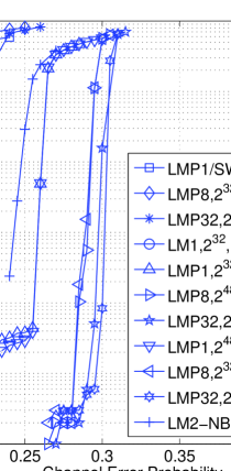
Figure 4: Simulation results for (3,6) regular codes with block length 100000.

Appendix A Proof of theorem II.1

Proof:

Given $p\lambda(1-\rho(1-x))<x$ for $x\in(0,1]$, we start by showing that both $x_{i}$ and $y_{i}$ go to zero as $i$ goes to infinity. To do this, we let $\alpha=\sup_{x\in(0,1)}\frac{1}{x}p\lambda(1-\rho(1-x))$ and note that $\alpha<1$ because $p<p^{*}$. It is also easy to see that, starting from $x_{0}=1$, we have $x_{i}\leq\alpha^{i}$ and $x_{i}\rightarrow 0$. Next, we rewrite (3) as

$$y_{i+1} =\frac{1}{p}x_{i+1}+p\left(\rho(1-x_{i})-\rho(1-y_{i})\right)\lambda^{\prime}(1-\rho(1-x_{i}))$$

$$\stackrel{{\scriptstyle(a)}}{{\leq}}\frac{1}{p}\alpha^{i+1}+p\left(1-\rho^{\prime}(1)\alpha^{i}-\rho(1-y_{i})\right)\left(\lambda_{2}+O(\alpha^{i})\right)$$

$$\stackrel{{\scriptstyle(b)}}{{\leq}}\frac{1}{p}\alpha^{i+1}+p\lambda(1-\rho(1-y_{i}))\left(1+O(\alpha^{i})\right)$$

$$\stackrel{{\scriptstyle(c)}}{{\leq}}\frac{1}{p}\alpha^{i+1}+\alpha y_{i}\left(1+O(\alpha^{i})\right),$$

where $(a)$ follows from $\rho(1-x)\leq 1-\rho^{\prime}(1)x$, $(b)$ follows from $\lambda_{2}(1-\rho(1-y))\leq\lambda(1-\rho(1-y))$, and $(c)$ follows from $p\lambda(1-\rho(1-y))\leq\alpha y$. It is easy to verify that $y_{i+1}<y_{i}$ as long as $y_{i}>\frac{\alpha^{i+1}}{p(1-\alpha(1+O(\alpha^{i})))}$. Therefore, we find that $y_{i}\rightarrow 0$ because the recursion does not have any positive fixed points as $i\rightarrow\infty$. Moreover, one can show that $y_{i}$ eventually decreases exponentially at a rate arbitrarily close to $\alpha$.

Now, we consider the performance of a randomly chosen code and with a random error pattern. The approach taken is general enough to cover all the message-based decoding algorithms discussed in this paper.

A message in the decoding graph is called bad if it is either unverified or falsely verified. Based on [15], one can show that, after $\ell$ decoding iterations, the fraction of bad messages is tightly concentrated around its average. We note that the concentration occurs regardless of whether there are falsely verified messages or short cycles. Since the proof involves no new techniques beyond [15] and the extension to irregular codes in [25], we give only a brief outline. The main difference between this scenario and [15] is that the algorithms discussed in this paper pass lists whose size may be unbounded and may be affected by FV. It turns out that the size of these lists is superfluous, however, if we only consider the fraction of messages satisfying a logical test (e.g., the fraction of bad messages).

Let the r.v. $Z^{(\ell)}$ denote the number of bad variable-to-check messages after $\ell$ iterations of decoding. Suppose the fraction of unverified messages predicted by DE, assuming no FV, is $y_{\ell}$. We say that concentration fails if $Z^{(\ell)}/E$ exceeds $y_{\ell}$ by more than $\epsilon$, where $E$ is the number of edges in the graph. Following [15], one can bound the failure probability by showing that the fraction of bad messages concentrates around its average value and that the average value converges to the value computed by DE.

The main observation is that the verification status of an edge, after $\ell$ iterations, depends only on the depth-$2\ell$ neighborhood, $\mathcal{N}_{\vec{e}}^{(2\ell)}$, of the directed edge $\vec{e}$. By using a Doob’s martingale for the edge-exposure process and applying Azuma’s inequality, one obtains the concentration bound

$$\Pr\left(\frac{Z^{(\ell)}}{E}-\frac{\mathbb{E}\left[Z^{(\ell)}\right]}{E}>\frac{\epsilon}{3}\right)\leq e^{-\beta_{\ell}\epsilon^{2}n},$$ (20)

where $\beta_{\ell}$ is a positive constant independent of $n$ which depends only on the d.d. and the number of iterations.

The next step is showing that the expected value $\mathbb{E}\left[Z^{(\ell)}\right]/E$ is close to the value, $y_{\ell}$, given by DE. In this case, we must consider two sources of error: short cycles and false verification. In [15] and [25], it is shown that, when a code graph is chosen uniformly at random from all possible graphs with degree distribution pair $(\lambda(x),\rho(x))$,

$$\Pr\left(\mathcal{N}_{\vec{e}}^{(2\ell)}\mbox{ is not tree-like}\right)\leq\frac{\gamma_{\ell}}{n},$$

where $\gamma_{\ell}$ is a constant independent of $n$ that depends only on the d.d. and number of iterations. So, for any $\epsilon>0$, one can choose $n$ large enough so that $\gamma_{\ell}/n<\epsilon/3$. Since type-II FV is a failure due to short cycles (see Section IV-B for details about type-I and type-II FV), this implies that any increase in $\mathbb{E}\left[Z^{(\ell)}\right]/E$ due to short cycles and type-II FV is at most $\epsilon/3$. Likewise, one can upper bound the effect of type-I FV with

$$\Pr\left(\mbox{any type-I FV occurred in }\mathcal{N}_{\vec{e}}^{(2\ell)}\right)\leq\frac{\theta_{\ell}}{q},$$

where $\theta_{\ell}$ is a constant independent of $n$ that depends only the d.d., the number of iterations, and algorithm details (e.g., $S_{max}$). If we choose $q$ large enough so that $\theta_{\ell}/q<\epsilon/3$, then these two bounds imply that

$$\frac{\mathbb{E}\left[Z^{(\ell)}\right]}{E}-y_{\ell}\leq\frac{\gamma_{\ell}}{n}+\frac{\theta_{\ell}}{q}\leq\frac{2\epsilon}{3}.$$ (21)

Finally, (20) and (21) can be combined to bound the probability that $Z^{(\ell)}/E$ is greater than $y_{\ell}+\epsilon$. ∎

Appendix B Proof of Lemma IV.1

Let $y$ be the received symbol sequence assuming the all-zero codeword was transmitted and let $u$ be another codeword with exactly $k$ non-zero symbols. Of the $k$ positions where they differ, assume that $i$ are received correctly, $j$ are flipped to other codeword’s value, and $k-i-j$ are flipped to a third value. It is easy to verify that the all-zero codeword is not the unique ML codeword whenever $i\leq j$. Therefore, the probability that ML decoder chooses $u$ over the all-zero codeword is given by

$$p_{2,k}=\sum_{j=0}^{k}\sum_{i=0}^{j}\textstyle\binom{k}{i,j,k-i-j}(1\!-\!p)^{i}\left(\frac{p}{q-1}\right)^{j}\left(\frac{p(q-2)}{q-1}\right)^{k-i-j}.$$

The multinomial theorem also shows that

$$A (x)=\textstyle\left((1\!-\!p)+\frac{p}{q-1}x^{2}+\frac{p(q-2)}{q-1}x\right)^{k}$$

$$=\displaystyle\sum_{j=0}^{k}\sum_{i=0}^{k-j}\textstyle\binom{k}{i,j,k-i-j}(1\!-\!p)^{i}\!\left(\frac{p}{q-1}\right)^{j}\!\left(\frac{p(q-2)}{q-1}\right)^{k-i-j}\!\!x^{k-i+j}$$

$$\triangleq\displaystyle\sum_{l=0}^{2k}A_{l}x^{l},$$

where $A_{l}$ is the coefficient of $x^{l}$ in $A(x)$. Next, we observe that $p_{2,k}=\sum_{l=k}^{2k}A_{l}$ is simply an unweighted sum of a subset of terms in $A(x)$ (namely, those where $k-i+j\geq k$).

This implies that

$$x^{k}p_{2,k}=\sum_{l=k}^{2k}A_{l}x^{k}\leq A(x)$$

for any $x\geq 1.$ Therefore, we can compute the Chernoff-type bound

$$p_{2,k}\leq\inf_{x\geq 1}x^{-k}A(x).$$

By taking derivative of $x^{-k}A(x)$ over $x$ and setting it to zero, we arrive at the bound

$$p_{2,k}\leq\left(p\frac{q-2}{q-1}+\sqrt{\frac{4p(1-p)}{q-1}}\right)^{k}.$$

Appendix C Proof of Lemma IV.3

Figure 5: Finite-state machine for Lemma IV.3.

Proof:

An unverification event occurs on a degree-2 cycle of length-$k$ when there is at most one correct variable node in any adjacent set of $s+1$ nodes. Let the set of all error patterns (i.e., 0 means correct and 1 means error) of length-$k$ which satisfy the UV condition be $\Phi(s,p,k)\subseteq\{0,1\}^{k}$. Using the Hamming weight $w(z)$, of an error pattern as $z$, to count the number of errors, we can write the probability of UV as

$$\phi(s,p,k)=\sum_{z\in\Phi(s,p,k)}p^{w(z)}(1-p)^{k-w(z)}.$$

This expression can be evaluated using the transfer matrix method to enumerate all weighted walks through a particular digraph. If we walk through the nodes along the cycle by picking an arbitrary node as the starting node, the UV constraint can be seen as $k$-steps of a particular finite-state machine. Since we are walking on a cycle, the initial state must equal to the final state.

The finite-state machine, which is shown in Fig. 5, has $s+1$ states $\{0,1,\ldots,s\}$. Let state 0 be the state where we are free to choose either a correct or incorrect symbol (i.e., the previous $s$ symbols are all incorrect). This state has a self-loop associated with the next symbol also being incorrect. Let state $i>0$ be the state where the past $i$ values consist of one correct symbol followed by $i-1$ incorrect symbols. Notice that only state 0 may generate correct symbols. By defining the transfer matrix with (19), the probability that the UV condition holds is therefore $\phi(s,p,k)=\textrm{Tr}\left(B^{k}(p)\right)$. ∎

Fan Zhang (S’03) received his Ph.D. in electrical engineering from Texas A&M University in 2010 and joined the read-channel arthitecture group at LSI Logic. He spent 3 years at UTStarcom Inc. before joining Texas A&M University. His current research interests include information theory, error correcting codes and signal processing for wireless and data storage systems.

Henry D. Pfister (S’99–M’03–SM’09) received his Ph.D. in electrical engineering from UCSD in 2003 and he joined the faculty of the School of Engineering at Texas A&M University in 2006. Prior to that he spent two years in R&D at Qualcomm, Inc. and one year as a post-doc at EPFL. He received the NSF Career Award in 2008 and was a coauthor of the 2007 IEEE COMSOC best paper in Signal Processing and Coding for Data Storage. His current research interests include information theory, channel coding, and iterative decoding with applications in wireless communications and data storage.

References

- [1] R. G. Gallager, “Low-density parity-check codes,” IRE Trans. Inform. Theory, vol. 18, pp. 21–28, Jan. 1962.
- [2] D. MacKay and R. Neal, “Good codes based on very sparse matrices,” Lecture Notes in Computer Science, vol. 1025, pp. 100–111, 1995.
- [3] M. Luby, M. Mitzenmacher, M. Shokrollahi, and D. Spielman, “Efficient erasure correcting codes,” IEEE Trans. Inf. Theory, vol. 47, pp. 569–584, Feb. 2001.
- [4] T. Richardson, M. Shokrollahi, and R. Urbanke, “Design of capacity-approaching irregular low-density parity-check codes,” IEEE Trans. Inf. Theory, vol. 47, pp. 619–637, Feb. 2001.
- [5] A. Shokrollahi, “Capacity-approaching codes on the -ary symmetric channel for large ,” in Proc. IEEE Inform. Theory Workshop, (San Antonio, TX), pp. 204–208, Oct. 2004.
- [6] C. Weidmann, “Coding for the -ary symmetric channel with moderate ,” in Proc. IEEE Int. Symp. Information Theory, July 2008.
- [7] G. Lechner and C. Weidmann, “Optimization of binary ldpc codes for the -ary symmetric channel with moderate ,” in Proc. 5th International Symposium on Turbo Codes and Related Topics, 2008.
- [8] M. Luby and M. Mitzenmacher, “Verification-based decoding for packet-based low-density parity-check codes,” IEEE Trans. Inf. Theory, vol. 51, pp. 120–127, Jan. 2005.
- [9] J. Metzner, “Majority-logic-like decoding of vector symbols,” IEEE Trans. Commun., vol. 44, pp. 1227–1230, Oct. 1996.
- [10] J. Metzner, “Majority-logic-like vector symbol decoding with alternative symbol value lists,” IEEE Trans. Commun., vol. 48, pp. 2005–2013, Dec. 2000.
- [11] M. Davey and D. MacKay, “Low density parity check codes over GF(),” IEEE Commun. Lett., vol. 2, pp. 58–60, 1998.
- [12] D. Bleichenbacher, A. Kiyayias, and M. Yung, “Decoding of interleaved Reed-Solomon codes over noisy data,” in Proc. of ICALP, pp. 97–108, 2003.
- [13] A. Shokrollahi and W. Wang, “Low-density parity-check codes with rates very close to the capacity of the -ary symmetric channel for large ,” in Proc. IEEE Int. Symp. Information Theory, (Chicago, IL), p. 275, June 2004.
- [14] A. Shokrollahi and W. Wang, “Low-density parity-check codes with rates very close to the capacity of the -ary symmetric channel for large .” Unpublished extended abstract, 2004.
- [15] T. Richardson and R. Urbanke, “The capacity of low-density parity-check codes under message-passing decoding,” IEEE Trans. Inf. Theory, vol. 47, pp. 599–618, Feb. 2001.
- [16] V. Guruswami and P. Indyk, “Linear time encodable and list decodable codes,” in Proc. of the 35th Annual ACM Symp. on Theory of Comp., pp. 126–135, 2003.
- [17] F. Zhang and H. D. Pfister, “On the stopping sets of verification decoding.” in preparation, June 2011.
- [18] N. Wormald, “Differential equations for random processes and random graphs,” Annals of Applied Probability, vol. 5, pp. 1217–1235, 1995.
- [19] F. Zhang and H. D. Pfister, “Software to compute the LM2-NB threshold.” at http://www.ece.tamu.edu/~hpfister/software/lm2nb_threshold.m.
- [20] N. C. Wormald, “The differential equation method for random graph processes and greedy algorithms,” in Lectures on Approximation and Randomized Algorithms, pp. 73–155, Polish Scientific Publishers, 1999.
- [21] T. J. Richardson and R. L. Urbanke, Modern Coding Theory. Cambridge University Press., 2008.
- [22] R. Storn and K. Price, “Differential evolution–A simple and efficient heuristic for global optimization over continuous spaces,” J. Global Optim., vol. 11, no. 4, pp. 341–359, 1997.
- [23] S. Sarvotham, D. Baron, and R. Baraniuk, “Sudocodes–Fast measurement and reconstruction of sparse signals,” in Proc. IEEE Int. Symp. Information Theory, (Seattle, WA), pp. 2804–2808, July 2006.
- [24] F. Zhang and H. D. Pfister, “Veri cation decoding of high-rate ldpc codes with applications in compressed sensing.” submitted to IEEE Trans. on Inform. Theory also available in Arxiv preprint cs.IT/0903.2232v3, 2009.
- [25] A. Kavcic, X. Ma, and M. Mitzenmacher, “Binary intersymbol interference channels: Gallager codes, density evolution, and code performance bounds,” IEEE Trans. Inf. Theory, vol. 49, pp. 1636–1652, July 2003.