Necessary and sufficient conditions for reflectionless transformation media in an isotropic and homogenous background

Abstract

It has been known that, keeping the outer boundary coordinates intact before and after a coordinate transformation is a sufficient condition for obtaining a reflectionless transformation medium. Here we prove that it is also a necessary condition for reflectionless transformation media in an isotropic and homogenous background. Our analytical results show that the outer boundary coordinates of a reflectionless transformation medium must be the same as the original coordinates with a combination of rotation and displacement, which is equivalent to situation that the boundary coordinates are kept intact before and after transformation.

1 Introduction

Recently, invisibility cloaks have received a lot of attentions [1]-[9], due to their amazing properties of excluding light from a protected object without perturbing exterior fields. The real breakthrough behind the story is the theoretical tools used to construct the cloak: transformation optics, in which coordinate transformation is applied to obtain a new set of permittivity and permeability tensors whereas Maxwell’s equations are still form invariant. Inspired by invisibility cloaks, different kinds of media constructed by the coordinate transformation method are proposed to control electromagnetic fields for novel applications, such as field concentrator [10], field shifter and splitter [11], field rotator [12], electromagnetic wormholes [13], and cylindrical superlens [15]. Such media obtained from the coordinate transformation are called as transformation media, in which the behaviors of light are determined by coordinate transformation functions.

For most of applications, it is desirable to have transformation media that are reflectionless to external light. It has been known that [1, 12, 14], keeping the outer boundary coordinates intact before and after a coordinate transformation is a sufficient condition for obtaining a reflectionless transformation medium. A strict proof has been given in Ref. [14]. However, it is still unclear that whether the condition is the only necessary condition for reflectionless transformation media, and whether other sufficient conditions exist for reflectionless transformation media. In the present paper, we analytically present the necessary and sufficient condition for reflectionless transformation media, in particular, in an isotropic and homogenous background medium. Some numerical examples are also given to confirm our findings.

2 Transformation media

Maxwell’s Equations without sources take the form as $\nabla\times{\bf E}=-\frac{{\partial{\bf B}}}{{\partial t}}$, $\nabla\times{\bf H}=\frac{{\partial{\bf D}}}{{\partial t}}$, $\nabla\cdot{\bf D}=0$, $\nabla\cdot{\bf B}=0$, with ${\bf D}=\overline{\overline{\varepsilon}}\cdot{\bf E}$, ${\bf B}=\overline{\overline{\mu}}\cdot{\bf H}$. Consider the transformation from the Cartesian coordinate system $(x,y,z)$ to an arbitrary curved coordinate system $(q_{1},q_{2},q_{3})$ (illustrated in Fig. 1), which can be described by a set of equations $x=f_{1}(q_{1},q_{2,}q_{3})$, $y=f_{2}(q_{1},q_{2,}q_{3})$, $z=f_{3}(q_{1},q_{2,}q_{3})$. Then Maxwell’s equations in the curved coordinate system can be expressed as $\nabla_{q}\times\widehat{\bf E}=-\frac{{\partial\widehat{\bf B}}}{{\partial t}}$, $\nabla_{q}\times\widehat{\bf H}=\frac{{\partial\widehat{\bf D}}}{{\partial t}}$, $\nabla_{q}\cdot\widehat{\bf D}=0$, $\nabla_{q}\cdot\widehat{\bf B}=0$, with $\widehat{\bf D}=\widehat{\overline{\overline{\varepsilon}}}\cdot\widehat{\bf E}$, $\widehat{\bf B}=\widehat{\overline{\overline{\mu}}}\cdot\widehat{\bf H}$, where

$$\widehat{\overline{\overline{\varepsilon}}}={{\det(g)}({g^{T}})^{-1}}{\overline{\overline{\varepsilon}}}g^{-1},\quad\widehat{\overline{\overline{\mu}}}={{\det(g)}({g^{T}})^{-1}}\widehat{\overline{\overline{\mu}}}g^{-1},$$ (1)

$$\widehat{\bf E}=g{\bf E},\quad\widehat{\bf H}=g{\bf H},$$ (2)

with

$$g=\left[{\begin{array}[]{*{20}c}{\frac{{\partial f_{1}}}{{\partial q_{1}}}}&{\frac{{\partial f_{2}}}{{\partial q_{1}}}}&{\frac{{\partial f_{3}}}{{\partial q_{1}}}}\\ {\frac{{\partial f_{1}}}{{\partial q_{2}}}}&{\frac{{\partial f_{2}}}{{\partial q_{2}}}}&{\frac{{\partial f_{3}}}{{\partial q_{2}}}}\\ {\frac{{\partial f_{1}}}{{\partial q_{3}}}}&{\frac{{\partial f_{2}}}{{\partial q_{3}}}}&{\frac{{\partial f_{3}}}{{\partial q_{3}}}}\\ \end{array}}\right].$$ (6)

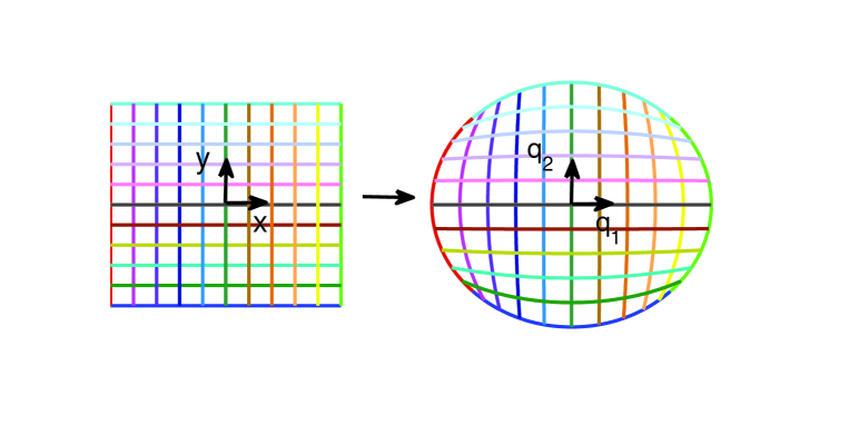
Figure 1: Illustration of coordinate transformation.

It is seen that Maxwell’s equations have the same form in any curved coordinate system. However, the permittivity and permeability change their values, which are expressed as the functions of $(q_{1},q_{2},q_{3})$ in Eq. 1. The media with such permittivity and permeability are thus transformation media, where $(q_{1},q_{2},q_{3})$ are treated as cartesian coordinates in physical space.

3 Necessary condition for reflectionless transformation media

Consider a transformation medium obtained by a coordinate transformation from a homogenous and isotropic background (e.g. vacuum) with permittivity $\epsilon$ and permeability $\mu$, and placed in the same medium.

To derive the necessary condition for reflectionless transformation media, we take the reflectionless property as a prerequisite. Since the incident waves can always be expressed as the superposition of the eigen waves, no reflection should occur for each eigen wave incidence. It is known that the eigen wave in a homogenous and isotropic medium is a plane wave. Consider an arbitrary propagating plane wave incident upon the transformation media. The boundary interacting with the incident wave between the transformation medium and surrounding medium (i.e., the original medium) is denoted by $S$. The electric and magnetic fields of the incident plane wave are denoted by

$${\bf E}_{i}(x,y,z)=\overline{\bf E}_{i}\exp(i{\bf k}_{i}\cdot{\bf r}),\,\,{\bf H}_{i}(x,y,z)=\overline{\bf H}_{i}\exp(i{\bf k}_{i}\cdot{\bf r}),$$ (7)

where $k_{i}=\omega\sqrt{\mu\varepsilon}$; $r=q_{1}\widehat{\bf x}+q_{2}\widehat{\bf y}+q_{3}\widehat{\bf z}$; $\overline{\bf E}_{i}$ and $\overline{\bf H}_{i}$ are constant vectors, representing the directions and magnitudes of electric and magnetic fields, respectively; $|\overline{\bf E}_{i}|/|\overline{\bf H}_{i}|=\sqrt{\mu/\varepsilon}$. Since the eigen waves in the transformation medium relate to those in the original medium, i.e., surrounding medium, by Eq. 2, the transmitted fields in the transformation medium can always be expressed as

$${\bf E}_{t}(q_{1},q_{2},q_{3})=\sum\limits_{n=-\infty}^{+\infty}{g\overline{\bf E}_{n}\exp(i{\bf k}_{n}\cdot{\bf r}^{{}^{\prime}})},\,\,{\bf H}_{t}(q_{1},q_{2},q)=\sum\limits_{n=-\infty}^{+\infty}{g\overline{\bf H}_{n}\exp(i{\bf k}_{n}\cdot{\bf r}^{{}^{\prime}})},$$ (8)

where $r^{{}^{\prime}}=f_{1}(q_{1,}q_{2,}q_{3})\widehat{\bf x}+f_{2}(q_{1,}q_{2,}q_{3})\widehat{\bf y}+f_{3}(q_{1,}q_{2,}q_{3})\widehat{\bf z}$; $\overline{\bf E}_{n}\exp(i{\bf k}_{n}\cdot{\bf r})$ and $\overline{\bf H}_{n}\exp(i{\bf k}_{n}\cdot{\bf r})$ represent the eigen plane waves in the surrounding medium, including both propagating and evanescent components.

Eq. 5 can also be rewritten as ${\bf E}_{t}(q_{1},q_{2},q_{3})=\exp(i{\bf k}_{i}\cdot{\bf r})\sum\limits_{n=-\infty}^{+\infty}{g\overline{\bf E}_{n}\exp[i({\bf k}_{n}\cdot{\bf r}^{{}^{\prime}}-{\bf k}_{i}\cdot{\bf r})]}$, ${\bf H}_{t}(q_{1},q_{2},q_{3})=\exp(i{\bf k}_{i}\cdot{\bf r})\sum\limits_{n=-\infty}^{+\infty}{g\overline{\bf H}_{n}\exp[i({\bf k}_{n}\cdot{\bf r}^{{}^{\prime}}-{\bf k}_{i}\cdot{\bf r})]}$. Boundary conditions for no reflection requires that the tangential components of ${\bf E}_{i}$ (${\bf H}_{i}$) and ${\bf E}_{t}$ (${\bf H}_{t}$) keep continuous across the boundary. To satisfy the boundary conditions, the phase factor of ${\bf E}_{i}$ and ${\bf H}_{i}$ at the boundary $S$, i.e., $\exp(i{\bf k}_{i}\cdot{\bf r_{S}})$, should be matched with the the phase factor of ${\bf E}_{t}$ and ${\bf H}_{t}$ at the same boundary. (Here the subscript $S$ indicates the values at the boundary.) Thus, ${\bf k}_{n}\cdot{\bf r_{S}}^{{}^{\prime}}-{\bf k}_{i}\cdot{\bf r_{S}}$ should be a constant at any points of the boundary $S$. While since ${\bf k}_{n}$ could have an arbitrary direction, at most one of ${\bf k}_{n}\cdot{\bf r_{s}}^{{}^{\prime}}-{\bf k}_{i}\cdot{\bf r_{s}}$ can be constant. It can then be concluded that only one term of $\overline{\bf E}_{n}$ ($\overline{\bf H}_{n}$) is non-zero, denoted by $\overline{\bf E}_{t}$ ($\overline{\bf H}_{t}$), while the other terms are all zeros. Now we have ${\bf E}_{t}=g\overline{\bf E}_{t}\exp(i{\bf k}_{t}\cdot{\bf r}^{{}^{\prime}}),\,\,{\bf H}_{t}(x,y,z)=g\overline{\bf H}_{t}\exp(i{\bf k}_{t}\cdot{\bf r}^{{}^{\prime}})$. It indicates that only one eigen wave is excited in the transformation medium for one specific incident eigen wave. The boundary conditions can then be written as

$$\widehat{\bf t}\cdot\overline{\bf E}_{i}\exp(i{\bf k}_{i}\cdot{\bf r_{S}})=\widehat{\bf t}\cdot g_{S}\overline{\bf E}_{t}\exp(i{\bf k}_{t}\cdot{\bf r_{S}}^{{}^{\prime}}),$$ (9)

$$\widehat{\bf t}\cdot\overline{\bf H}_{i}\exp(i{\bf k}_{i}\cdot{\bf r_{S}})=\widehat{\bf t}\cdot g_{S}\overline{\bf H}_{t}\exp(i{\bf k}_{t}\cdot{\bf r_{S}}^{{}^{\prime}}),$$ (10)

where $\widehat{\bf t}$ represents the unit vector in the tangential direction of the boundary $S$. The phase matching requires that

$${\bf k}_{i}\cdot{\bf r_{S}}={\bf k}_{t}\cdot{\bf r_{S}}^{{}^{\prime}}+\phi,$$ (11)

where $\phi$ is a constant.

Since the incident eigen wave $\{\overline{\bf E}_{i}\exp(i{\bf k}_{i}\cdot{\bf r}),\overline{\bf H}_{i}\exp(i{\bf k}_{i}\cdot{\bf r})\}$ is a propagating plane wave, $\{\overline{\bf E}_{t}\exp(i{\bf k}_{t}\cdot{\bf r}),\overline{\bf H}_{t}\exp(i{\bf k}_{t}\cdot{\bf r})\}$ should also be the propagating plane wave for the conservation of energy through the boundary. The unit vectors in the directions of $\overline{\bf E}_{t}$, $\overline{\bf H}_{t}$, and ${\bf k}_{t}$ are denoted by $\widehat{\bf e}_{t}^{1}$, $\widehat{\bf e}_{t}^{2}$ and $\widehat{\bf e}_{t}^{3}$, which are orthogonal to each other. While the unit vectors in the directions of $\overline{\bf E}_{i}$, $\overline{\bf H}_{i}$, and ${\bf k}_{i}$ are denoted by $\widehat{\bf e}_{i}^{1}$, $\widehat{\bf e}_{i}^{2}$ and $\widehat{\bf e}_{i}^{3}$, which are also orthogonal to each other. It is obvious that $({\widehat{\bf e}_{t}^{1},\widehat{\bf e}_{t}^{2},\widehat{\bf e}_{t}^{3}})$ can be coincident with $({\widehat{\bf e}_{i}^{1},\widehat{\bf e}_{i}^{2},\widehat{\bf e}_{i}^{3}})$ after a certain rotation, where a ${3\times 3}$ orthogonal matrix $R$ can be defined to characterize this rotation, with ${\bf e}_{t}^{j}=R{\bf e}_{i}^{j}$ $(j=1,2,3)$. Therefore, ${\bf E}_{t}$ and ${\bf H}_{t}$ can be expressed as

$$\;\;\;\;\;\;\;\;\;\;\;{\bf E}_{t}=gR^{-1}q\overline{\bf E}_{i}\exp(i{\bf k}_{i}\cdot R{\bf r}^{{}^{\prime}}),\,\,{\bf H}_{t}(x,y,z)=gR^{-1}q\overline{\bf H}_{i}\exp(i{\bf k}_{i}\cdot R{\bf r}^{{}^{\prime}}),$$ (12)

where $q$ is a constant, and $R^{-1}$ is the inversion of $R$. The phase matching condition at the boundary expressed in Eq. 8 can thus be written as

$${\bf k}_{i}\cdot{\bf r_{S}}={\bf k}_{i}\cdot R{\bf r_{S}}^{{}^{\prime}}+\phi,$$ (13)

which requires ${\bf r_{s}}-R{\bf r_{s}}^{{}^{\prime}}$ to be a constant vector, i.e.,

$${\bf r_{S}}=R{\bf r_{S}}^{{}^{\prime}}+{\bf u},$$ (14)

where ${\bf u}$ denoted by ${\bf u}=u_{1}\widehat{\bf x}+u_{2}\widehat{\bf y}+u_{3}\widehat{\bf z}$ is a constant vector, and $\phi={\bf k}_{i}\cdot{\bf u}$. Eq. 14 is the necessary condition for reflectionless transformation media, resulted from the requirement of phase matching at the boundary.

4 Sufficient condition for reflectionless transformation media

In this section, we briefly prove that Eq. 11 is also the sufficient condition for reflectionless transformation media. Consider a propagating plane wave ${\bf E}_{i}$ and ${\bf H}_{i}$ expressed in Eq. (4) incident upon the transformation medium, whose outer boundary coordinates $\bf r_{S}$ are related to the transformed coordinates $\bf r^{{}^{\prime}}_{S}$ by Eq. 11. The the transmitted fields ${\bf E}_{t}$ and ${\bf H}_{t}$ in the transformation medium are directly obtained by the coordinate transformation through Eq. 9, which satisfy Maxwell’s equations in the transformation medium. Below we will show that the tangential fields of the incident wave in Eq. 4 equal to the tangential fields of the transmitted fields in Eq. 9, which means the transformation medium is reflectionless.

From Eq. 11, we can obtain ${\bf r_{S}}^{{}^{\prime}}=R^{-1}({\bf r_{S}}-{\bf u})=R^{T}({\bf r_{S}}-{\bf u})$, where the superscript ”$T$” denotes the transpose of matrix. Here, it is noted that $R^{-1}=R^{T}$ since $R$ is an orthogonal matrix. Because ${\bf r_{s}}^{{}^{\prime}}=f_{1}(q_{1,}q_{2,}q_{3})\widehat{\bf x}+f_{2}(q_{1,}q_{2,}q_{3})\widehat{\bf y}+f_{3}(q_{1,}q_{2,}q_{3})\widehat{\bf z}$, we have $f_{j}(q_{1},q_{2},q_{3})=R_{1j}(q_{1}-u_{1})+R_{2j}(q_{2}-u_{2})+R_{3j}(q_{3}-u_{3})$ $(j=1,2,3)$. It is obvious that $\nabla_{q}f_{j}-\nabla_{q}[R_{1j}(q_{1}-u_{1})+R_{2j}(q_{2}-u_{2})+R_{3j}(q_{3}-u_{3})]$, i.e., $(\partial f_{j}/\partial q_{1}-R_{1j})\widehat{\bf x}+(\partial f_{j}/\partial q_{2}-R_{2j})\widehat{\bf y}+(\partial f_{j}/\partial q_{3}-R_{3j})\widehat{\bf z}$, lie in the same line as the normal direction of $S$. Therefore, $g_{S}$ can be expressed as

$$g_{S}=[F_{1}{\widehat{\bf n}},\;F_{2}\widehat{\bf n},\;F_{3}\widehat{\bf n}]+R,$$ (15)

where $\widehat{\bf n}$ is the unit vector in the normal direction of the boundary $S$; $F_{j}\widehat{\bf n}=(\partial f_{j}/\partial q_{1}-R_{1j})\widehat{\bf x}+(\partial f_{j}/\partial q_{2}-R_{2j})\widehat{\bf y}+(\partial f_{j}/\partial q_{3}-R_{3j})\widehat{\bf z}$. Then, we obtain that $g_{S}R^{-1}=[F_{1}{\widehat{\bf n}},\;F_{2}\widehat{\bf n},\;F_{3}\widehat{\bf n}]R^{-1}+diag[1,1,1]$, and

$$\widehat{\bf t}\cdot g_{s}R^{-1}=\widehat{\bf t}.$$ (16)

Observing Eqs. 4, 9 and 13, it is obvious that, at the boundary $S$,

$$\widehat{\bf t}\cdot{\bf E}_{i}=\widehat{\bf t}\cdot{\bf E}_{t},\;\widehat{\bf t}\cdot{\bf H}_{i}=\widehat{\bf t}\cdot{\bf H}_{t},$$ (17)

with $q=\exp(i{\bf k_{i}}\cdot{\bf u})$. Eq. 14 means that ${\bf E}_{i}$ (${\bf H}_{i}$) and ${\bf E}_{t}$ (${\bf H}_{t}$) keep continuous across the boundary $S$, i.e., no reflection is excited for any propagating eigen wave incidence if Eq. 11 is satisfied. In conclusion, Eq. 11 is the sufficient condition for a reflectionless transformation medium in a homogenous and isotropic surrounding medium.

Here, it should be noted the derived condition in Eq. 11 is for the boundary, on which the transformation medium interacts with the incident waves simultaneously. If the transformation medium has sperate boundaries, which interact with waves in a certain sequence. A simple example is a slab structure having two separate boundaries for an incident wave from on side of the slav (see Ref. [11]). For such separate boundaries, the condition in Eq. 11 can be satisfied independently, i.e., different boundaries have different $R$ and ${\bf u}$ to satisfy Eq. (11). Therefore, if part of the boundary satisfies the condition and the waves incident mainly upon this part, the overall scattering (reflection) could be negligible. This well explained the mechanism of the reflectionless design in Ref. [11] in a more strict sense. In particular, the reflectionless condition expressed in Ref. [11] is that the distances measured along the $x$, $y$ and $z$ in the transformation medium and free space must be equal along the boundary, where the boundary is in $y-z$ plane.This equally measured distances in the transformation medium and free space indicates that the coordinates can be the same before and after transformation after a certain displacement. In fact, the distance measured along the $x$, i.e., the direction normal to the boundary, needn’t be equal along the boundary. The reason is that the boundary is in $y-z$ plane and a displacement in $x$ direction can always be found to make the boundary coordinates of $x$ component be the same before and after transformation, only if the boundary coordinates of $x$ component transform to the same value via coordinate transformation.

Furthermore, let us consider a rotation $R$ and a displacement ${\bf u}$ operating on the coordinates $(x,y,z)$ in the original isotropic and homogenous space before the coordinate transformation. The new coordinates after rotation $R$ and displacement ${\bf u}$ are denoted by $(x^{{}^{\prime}},y^{{}^{\prime}},z{{}^{\prime}})$. Since the medium is isotropic and homogenous, eigen waves are the same under the new coordinates. The boundary coordinates of the region to be transformed is now changed from ${\bf r_{S}}^{{}^{\prime}}$ to $R{\bf r_{S}}^{{}^{\prime}}+{\bf u}$ denoted by ${\bf r_{S}}^{{}^{\prime\prime}}$, which is the same as the right term of Eq. 11. Thus, the transformation medium can be considered as being constructed by transformation from $(x^{{}^{\prime}},y^{{}^{\prime}},z{{}^{\prime}})$ to $(q_{1},q_{2},q_{3})$, with the boundary coordinates keep intact before and after transformation, i.e.,

$${\bf r_{s}}={\bf r_{s}}^{{}^{\prime\prime}}.$$ (18)

Therefore, in the case of an isotropic and homogenous background, the necessary and sufficient condition expressed in Eq. 11 is equivalent to the condition that coordinates of the boundary are kept the same before and after transformation.

5 Numerical examples

To illustrate the above derived condition clearly, we present some numerical examples here. In Fig. 2 (a), a transformation of compressing a cylindrical region of free space with $x=2q_{1}$ and $y=2q_{2}$ is shown. The corresponding transformation medium has the parameters $\widehat{\overline{\overline{\epsilon}}}=\widehat{\overline{\overline{\mu}}}=diag[1,1,4]$. The corresponding electric field distribution for a line current source interacting with such obtained transformation media, is plotted in Fig. 2(b). It is clearly seen that reflections and hence scatterings are excited, since the boundary coordinates can’t be kept the same before and after transformation by rotation and displacement. In Fig. 3(a1) and (a2), the transformations of a elliptic region into an elliptic annular region are shown. The outer boundary coordinates are kept intact before and after transformation for (a1), while the outer boundary coordinates can be kept the same by rotation and displacement for (a2). Such transformation is operated under free space background. The obtained transformation media are elliptic invisibility cloaks. The electric field distributions under a line current source for (a1) and (a2) are plotted in (b1) and (b2), where we see no reflection is excited since Eq. 11 can be satisfied for both cases.

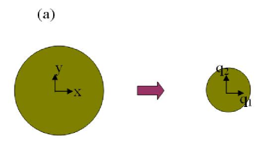
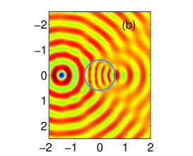
Figure 2: (a) Coordinate transformation of compressing a cylindrical region; (b) Electric field distribution for a line current source interacting with the obtained transformation medium. The transformation is operated under a free space background.

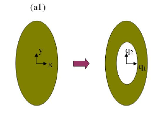
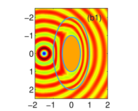
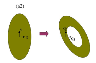
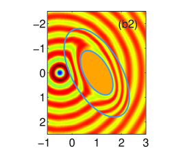
Figure 3: (a1) and (a2) Coordinate transformations of a elliptic region into a elliptic annular region; (b1) and (b2) Electric field distribution for a line current source interacting with the transformation media (a1) and (a2), respectively. The transformation is operated under a free space background.

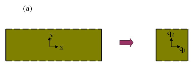
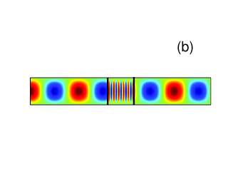
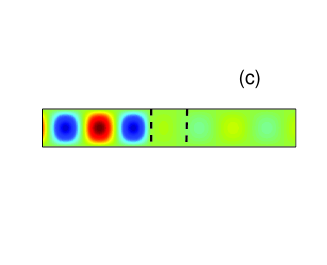
Figure 4: (a) Coordinate transformation of compressing a rectangular region into a square region. The compression is only done in $x$ direction. The left and right boundaries are denoted by solid lines, and the up and down boundaries are denoted by dash lines. Electric field distribution when the obtained transformation media is put in a PEC waveguide for (b) the left and right sides of the transformation medium interacting with the waves (c) the up and down sides of the transformation medium interacting with the waves. The transformation is operated under a free space background.

As discussed in the above, if one part of the boundary satisfies the condition and the waves incident mainly upon this part, reflection might be negligible. Consider a transformation illustrated in Fig. 4(a), where a rectangular region of free space is transformed into a square region, by compressing the space only in $x$ direction. The coordinates of the left and right boundaries denoted by solid lines can be kept the same before and after transformation by displacement. However, the coordinates of the up and down boundaries denoted by dashed lines can’t be kept the same after transformation by rotation and displacement. Put such square transformation medium in a PEC (Perfectly Electrical Conductor) waveguide. The wave behaviors in the waveguide are illustrated in Fig. 4(b) and (c). In Fig. 4(b), the waves only interact with the left and right boundaries of the transformation medium in the propagation direction. Thus, no reflection is observed. However, in Fig. 4(c), the waves interact with the up and down boundaries of the transformation medium, where reflections are excited.

6 Discussions and conclusions

In conclusion, we derived the necessary and sufficient condition for a reflectionless transformation medium in an isotropic and homogenous surrounding medium in this paper. The geometrical expression of this condition is that the transformed coordinates of the boundary can be the same as the original coordinates only by rotation and displacement of the coordinates. In a general sense, this condition is equivalent to the condition that the boundary coordinates are kept the same before and after transformation. Numerical simulations confirmed our findings.

References

References

• [1] Pendry J B, Schurig D, and Smith D R 2006 Science 312 1780.
• [2] Leonhardt U 2006 Science 312 1777
• [3] Cummer S A, Popa B I, Schurig D, Smith D R, and Pendry J B 2006 Phys. Rev. E. 74 036621
• [4] Zolla F, Guenneau S, Nicolet A, and Pendry J B 2007 Opt. Lett. 32 1069
• [5] Chen H S, Wu B I, Zhang B L, and Kong J A 2007 Phys. Rev. Lett. 99 063903
• [6] Ruan Z C, Yan M, Neff C W, and Qiu M 2007 Phys. Rev. Lett. 99 113903
• [7] Schurig D, Mock J J, Justice B J, Cummer S A, Pendry J B, Starr A F, and Smith D R 2006 Science 314 977
• [8] Greenleaf A, Kurylev Y, Lassas M and Uhlmann G 2007 Opt. Express 15 12717
• [9] Leonhardt U 2006 New J. Phys. 8 247
• [10] Rahm M, Schurig D, Roberts D A, Cummer S A, Smith D R and Pendry J B 2008 Photon. Nanostruct.: Fundam. Applic. 6 87
• [11] Rahm M, Cummer S A, Schurig D, Pendry J B, and Smith D R 2008 Phys. Rev. Lett. 100 063903
• [12] Chen H Y and Chan C T 2007 Appl. Phys. Lett. 90 241105
• [13] Greenleaf A, Kurylev Y, Lassas M, and Uhlmann G 2007 Phys. Rev. Lett. 99 183901
• [14] Yan W, Yan M, Ruan Z C, and Qiu M 2008 New J. Phys. 10 043040
• [15] Yan M, Yan W, and Qiu M 2008 //www.arXiv:0804.2850[physics.optics]