HIP-2008-20/TH

The lightest Higgs boson mass in effective field theory with bulk and brane supersymmetry breaking

Nobuhiro Uekusa

Department of Physics, University of Helsinki
and Helsinki Institute of Physics,
P.O. Box 64, FIN-00014 Helsinki, Finland

E-mail: nobuhiro.uekusa@helsinki.fi

We study the mass of the lightest Higgs boson in an effective Kaluza-Klein theory with two sources of supersymmetry breaking. When stop mass matrices are non-diagonal with respect to Kaluza-Klein modes and each element is not small in unit of the inverse compactification radius, a very small eigenvalue can be accommodated in the diagonalized basis. We show that in the model with the two sources, the Higgs boson mass can receive suitable corrections for various compactification radii.

1 Introduction

There has been much attention to the values of the masses of Higgs bosons. The Higgs field of the Standard Model has a classical potential composed of quadratic and quartic self-couplings. The mass receives radiative corrections from loop diagrams. If the Higgs field couples to a fermion with a dimensionless Yukawa coupling constant and an ultraviolet moment cutoff is employed to regulate the loop integral, the correction to the mass squared yields a quadratic term of the cutoff. There are similar contributions from the virtual effects of heavy fields, as emphasized in the introduction [1]. When there is a heavy complex scalar field $\Phi$ coupled to the Higgs field $H$ with the coupling $-\lambda_{\Phi}|H|^{2}|\Phi|^{2}$, the Higgs field receives a correction to the squared mass dependent on the cutoff,

$$\Delta m_{H}^{2}={\lambda_{\Phi}\over 16\pi^{2}}\left[\Lambda^{2}-2m_{\Phi}^{2}\textrm{ln}\left({\Lambda\over m_{\Phi}}\right)\right].$$ (1.1)

In addition to a quadratic term of the ultraviolet momentum cutoff $\Lambda$, there is a quadratic term of the heavy field mass $m_{\Phi}$. Heavy fermions also contribute similar corrections. In the light of the sensitivity of the Higgs boson mass to the masses of heavy fields, the effects on the Standard Model are not decoupled to heavy fields.

Once supersymmetry is assumed, such terms sensitive to the ultraviolet momentum cutoff and heavy field masses are canceled between bosonic and fermionic contributions. Because superparticles have not been detected, supersymmetry must be broken. In order to keep cancellation of the quadratic term on the cutoff, supersymmetry breaking needs to be soft. After supersymmetry is broken, the divergent correction to the Higgs boson mass squared is of a logarithmic form

$$\Delta m_{H}^{2}=m_{\textrm{\scriptsize sp}}^{2}\left[{\lambda\over 16\pi^{2}}\ln\left({\Lambda\over m_{\textrm{\scriptsize sp}}}\right)\right].$$ (1.2)

Here $m_{\textrm{\scriptsize sp}}$ is the largest mass scale associated with the mass splittings between bosons and fermions and $\lambda$ stands for dimensionless couplings schematically. In the Minimal Supersymmetric Standard Model (MSSM) with $\Lambda$ of the Planck scale and $\lambda$ of order ${\cal O}(1)$, the $m_{\textrm{\scriptsize sp}}$ is at the most 1 TeV so that the correction $\Delta m_{H}^{2}$ is not too large compared to the electroweak breaking scale.

To achieve mass splittings is of great interest in its own right. Supersymmetry must be broken in a way with no supersymmetric flavor problem. One candidate is to spatially separate the MSSM fields from the source of supersymmetry breaking [2]-[5], as the mediation in bulk spacetime does not distinguish flavor. When the radius of an extra dimension is denoted as $R$, the mass splitting between a bulk field and its supersymmetric partner can be of the order of $R^{-1}$ with a factor of order ${\cal O}(1)$. This type of mass splitting is obtained by $F$-term supersymmetry breaking on a brane [2][6]-[8] or independently by Scherk-Schwarz supersymmetry breaking [9]-[20]. If $R^{-1}\sim$ 1 TeV, corrections to the Higgs mass would be significant. In a Kaluza-Klein approach, bulk fields are decomposed in zero mode and Kaluza-Klein modes. Kaluza-Klein modes contain many heavy fields and each provides corrections of the form given in Eq. (1.1). In models with softly broken supersymmetry, corrections would have the form (1.2). Here each of Kaluza-Klein modes as well as zero mode acquires the mass splitting between bosonic and fermionic fields. Because the contribution from each mode is summed, supersymmetry breaking with extra dimensions may increase the corrections to Higgs boson masses. In the context of extra dimensions, effective potentials and Higgs boson masses have been widely studied [8][21]-[35].

Both of the two ways of supersymmetry breaking above can provide the mass splitting of the same order. On the other hand, there is a difference about the structure of Kaluza-Klein mode between them. For the Scherk-Schwarz supersymmetry breaking, supersymmetry-breaking mass matrices in the Lagrangian are diagonal with respect to Kaluza-Klein mode and $F$-term supersymmetry breaking on a brane leads to non-diagonal supersymmetry-breaking mass matrices. In the latter case each component of the mass matrices is of the order of $R^{-1}$ and in the diagonalized basis the eigenvalues are also of the order of $R^{-1}$.

In the case with the Scherk-Schwarz twist, $N=1$ supersymmetry can be locally preserved on each boundary. Thus supersymmetric action can be given at each boundary and it may be locally broken by some brane effects. Such a combined supersymmetry breaking is physically inequivalent to that of only one supersymmetry-breaking source because of distinct mass spectrum. However, its possibility has not been considered in the literature. A point to be examined is whether supersymmetry-breaking mass matrices assembled of the two possible sources about of order ${\cal O}(1)$ can give rise to at least one small eigenvalue in the diagonalized basis. If very small eigenvalues are generated, the effect of radiative corrections might be too small contributions to explain the Higgs boson mass in an allowed region for $R^{-1}\sim 1$ TeV. Instead it may be possible that the resulting Higgs mass amounts to being corrected for a large $R^{-1}$ such as the grand unification scale due to the mass splitting made of $R^{-1}$ multiplied by the small factor.

We study the corrections to the mass of the lightest Higgs boson in a Kaluza-Klein effective field theory. In a simple model, it is explicitly shown how the contribution from the mass splitting of each Kaluza-Klein level is summed. In a model with supersymmetry broken by Scherk-Schwarz twists and $F$-terms on a brane, we find that small eigenvalues for mass matrices can be accommodated. We show that for the two supersymmetry-breaking sources, quantum loop corrections with a variety of compactification scales can relax the upper bound to the mass of the lightest Higgs boson.

The paper is organized as follows. In Section 2, our notation for the lightest Higgs boson is given. In Section 3, a picture for obtaining radiative corrections to the lightest Higgs boson is shown for the four-dimensional case and Kaluza-Klein case. In Section 4, our model with Scherk-Schwarz twists and boundary $F$-term is presented. We calculate the diagonalization of mass matrices with respect to Kaluza-Klein modes. A conclusion is made in Section 5.

2 The Higgs bosons in a mass-eigenstate basis

In this section, we summarize our notation for the lightest Higgs boson following Ref. [1, 36]. The Higgs scalar fields in the MSSM consist of two complex SU(2)_L-doublets $H_{1}$ and $H_{2}$ which in total have 8 real scalar degrees of freedom

$$H_{1} \!\!\!=\!\!\! \left(\begin{array}[]{c}H_{1}^{0}\\ H_{1}^{-}\\ \end{array}\right)=\left(\begin{array}[]{c}H_{d}^{0}\\ H_{d}^{-}\\ \end{array}\right),\qquad(1,2,-\textrm{${1\over 2}$}),$$ (2.5)

$$H_{2} \!\!\!=\!\!\! \left(\begin{array}[]{c}H_{2}^{+}\\ H_{2}^{0}\\ \end{array}\right)=\left(\begin{array}[]{c}H_{u}^{+}\\ H_{u}^{0}\\ \end{array}\right),\qquad(1,2,+\textrm{${1\over 2}$}).$$ (2.10)

Here the quantum numbers for SU(3)$\times$ SU(2)_L $\times$ U(1)_Y are indicated by the numbers in the parentheses. The superpartners are the spin 1/2 higgsinos

$$\left(\begin{array}[]{c}\tilde{H}_{1}^{0}\\ \tilde{H}_{1}^{-}\\ \end{array}\right),~{}\left(\begin{array}[]{c}\tilde{H}_{2}^{+}\\ \tilde{H}_{2}^{0}\\ \end{array}\right).$$ (2.15)

We express the superpartners of the Standard Model fields by putting a tilde on the corresponding letter. The potential of the Higgs scalar fields is

$$V \!\!\!=\!\!\! (|\mu|^{2}+m_{1}^{2})|H_{1}|^{2}+(|\mu|^{2}+m_{2}^{2})|H_{2}|^{2}+\left[bH_{1}H_{2}+\textrm{H.c.}\right]$$ (2.16)

$$+{1\over 8}g^{2}(H_{2}^{\dagger}\sigma^{a}H_{2}+H_{1}^{\dagger}\sigma^{a}H_{1})^{2}+{1\over 8}g^{\prime}{}^{2}(|H_{2}|^{2}-|H_{1}|^{2})^{2}$$

$$\!\!\!=\!\!\! (|\mu|^{2}+m_{1}^{2})(|H_{1}^{0}|^{2}+|H_{1}^{-}|^{2})+(|\mu|^{2}+m_{2}^{2})(|H_{2}^{+}|^{2}+|H_{2}^{0}|^{2})$$

$$+\left[b(H_{1}^{-}H_{2}^{+}-H_{1}^{0}H_{2}^{0})+\textrm{H.c.}\right]$$

$$+{1\over 8}(g^{2}+g^{\prime}{}^{2})(|H_{2}^{+}|^{2}+|H_{2}^{0}|^{2}-|H_{1}^{0}|^{2}-|H_{1}^{-}|^{2})^{2}+{1\over 2}g^{2}|H_{2}^{+}H_{1}^{0*}+H_{2}^{0}H_{1}^{-*}|^{2},$$

where $g$ and $g^{\prime}$ denote SU(2)_L and U(1)_Y gauge coupling constants, respectively, $\mu$ is a supersymmetric mass and $m_{1}$, $m_{2}$ and $b$ are supersymmetry-breaking coupling constants.

For $H_{2}^{+}=H_{1}^{-}=0$, the Higgs potential is

$$V \!\!\!=\!\!\! (|\mu|^{2}+m_{1}^{2})|H_{1}^{0}|^{2}+(|\mu|^{2}+m_{2}^{2})|H_{2}^{0}|^{2}-\left[bH_{1}^{0}H_{2}^{0}+\textrm{H.c.}\right]$$ (2.17)

$$+{1\over 8}(g^{2}+{g^{\prime}}^{2})(|H_{2}^{0}|^{2}-|H_{1}^{0}|^{2})^{2}.$$

The equilibrium conditions $\partial V/\partial H_{2}^{0}=\partial V/\partial H_{1}^{0}=0$ at $H_{1}^{0}=v_{1},H_{2}^{0}=v_{2}$ lead to

$$|\mu|^{2}+m_{2}^{2}-b\cot\beta-(m_{Z}^{2}/2)\cos 2\beta=0,$$ (2.18)

$$|\mu|^{2}+m_{1}^{2}-b\tan\beta+(m_{Z}^{2}/2)\cos 2\beta=0,$$ (2.19)

respectively. Here

$$\tan\beta={v_{2}\over v_{1}},\quad m_{W}^{2}={1\over 2}g^{2}(v_{1}^{2}+v_{2}^{2}),\quad m_{Z}^{2}={1\over 2}(g^{2}+{g^{\prime}}^{2})(v_{1}^{2}+v_{2}^{2}).$$ (2.20)

Eqs. (2.18) and (2.19) require

$$b^{2}>(|\mu|^{2}+m_{1}^{2})(|\mu|^{2}+m_{2}^{2}).$$ (2.21)

When the electroweak symmetry is broken, three among the eight degrees of freedom of the Higgs scalar fields are the would-be Nambu-Goldstone bosons $G^{0}$ and $G^{\pm}$ which become the longitudinal modes of the $Z^{0}$ and $W^{\pm}$ massive vector bosons. The remaining five eigenstates are classified in three electrically-neutral fields and two electrically-charged fields. Electrically-neutral fields consist of two CP-even scalars $h^{0}$ and $H^{0}$ and one CP-odd scalar $A^{0}$. Electrically-charged fields are one scalar $H^{+}$ with charge $+1$ and its conjugate scalar $H^{-}$ with charge $-1$. Here $h^{0}$ is lighter than $H^{0}$. The charged scalars are subject to $G^{-}=G^{+*}$, $H^{-}=H^{+*}$. The gauge-eigenstate fields can be expressed in terms of the mass-eigenstate fields as

$$\left(\begin{array}[]{c}H_{2}^{0}\\ H_{1}^{0}\\ \end{array}\right)=\left(\begin{array}[]{c}v_{2}\\ v_{1}\\ \end{array}\right)+{1\over\sqrt{2}}R_{\alpha}\left(\begin{array}[]{c}h^{0}\\ H^{0}\\ \end{array}\right)+{i\over\sqrt{2}}R_{\beta_{0}}\left(\begin{array}[]{c}G^{0}\\ A^{0}\\ \end{array}\right),$$ (2.30)

$$\left(\begin{array}[]{c}H_{2}^{+}\\ H_{1}^{-*}\\ \end{array}\right)=R_{\beta_{\pm}}\left(\begin{array}[]{c}G^{+}\\ H^{+}\\ \end{array}\right).$$ (2.35)

The rotation matrices are given by

$$R_{\alpha}=\left(\begin{array}[]{cc}\cos\alpha&\sin\alpha\\ -\sin\alpha&\cos\alpha\\ \end{array}\right),~{}~{}R_{\beta_{0}}=\left(\begin{array}[]{cc}\sin\beta_{0}&\cos\beta_{0}\\ -\cos\beta_{0}&\sin\beta_{0}\\ \end{array}\right),$$ (2.40)

$$R_{\beta_{\pm}}=\left(\begin{array}[]{cc}\sin\beta_{\pm}&\cos\beta_{\pm}\\ -\cos\beta_{\pm}&\sin\beta_{\pm}\\ \end{array}\right).$$ (2.43)

The electrically-neutral part of the potential is

$$V^{\textrm{\scriptsize neutral}}={1\over 2}m_{h^{0}}^{2}{h^{0}}^{2}+{1\over 2}m_{H^{0}}^{2}{H^{0}}^{2}+{1\over 2}m_{G^{0}}^{2}{G^{0}}^{2}+{1\over 2}m_{A^{0}}^{2}{A^{0}}^{2},$$ (2.44)

with $\textrm{diag}(m_{h^{0}}^{2},m_{H^{0}}^{2})=R^{-1}_{\alpha}m_{\phi_{R}^{0}}^{2}R_{\alpha}$, $\textrm{diag}(m_{G^{0}}^{2},m_{A^{0}}^{2})=R^{-1}_{\beta_{0}}m_{\phi_{I}^{0}}^{2}R_{\beta_{0}}$. Here

$$m_{\phi_{R}^{0}}^{2} \!\!\!=\!\!\! \left(\begin{array}[]{cc}|\mu|^{2}+m_{2}^{2}+{g^{2}+{g^{\prime}}^{2}\over 4}(3v_{2}^{2}-v_{1}^{2})&-b-{g^{2}+{g^{\prime}}^{2}\over 2}v_{1}v_{2}\\ -b-{g^{2}+{g^{\prime}}^{2}\over 2}v_{1}v_{2}&|\mu|^{2}+m_{1}^{2}+{g^{2}+{g^{\prime}}^{2}\over 4}(3v_{1}^{2}-v_{2}^{2})\end{array}\right),$$ (2.47)

$$m_{\phi_{I}^{0}}^{2} \!\!\!=\!\!\! \left(\begin{array}[]{cc}|\mu|^{2}+m_{2}^{2}+{g^{2}+{g^{\prime}}^{2}\over 4}(v_{2}^{2}-v_{1}^{2})&b\\ b&|\mu|^{2}+m_{1}^{2}+{g^{2}+{g^{\prime}}^{2}\over 4}(v_{1}^{2}-v_{2}^{2})\end{array}\right).$$ (2.50)

The electrically-charged part of the potential is

$$V^{\textrm{\scriptsize charged}}=m_{G^{\pm}}^{2}G^{+}G^{-}+m_{H^{\pm}}^{2}H^{+}H^{-},$$ (2.51)

with $\textrm{diag}(m_{G^{\pm}}^{2},m_{H^{\pm}}^{2})=R^{-1}_{\beta_{\pm}}m_{\phi^{\pm}}^{2}R_{\beta_{\pm}}$. Here

$$m_{\phi^{\pm}}^{2}=\left(\begin{array}[]{cc}|\mu|^{2}+m_{2}^{2}+{g^{2}+{g^{\prime}}^{2}\over 4}v_{2}^{2}+{g^{2}-{g^{\prime}}^{2}\over 4}v_{1}^{2}&b+{g^{2}\over 2}v_{1}v_{2}\\ b+{g^{2}\over 2}v_{1}v_{2}&|\mu|^{2}+m_{1}^{2}+{g^{2}+{g^{\prime}}^{2}\over 4}v_{1}^{2}+{g^{2}-{g^{\prime}}^{2}\over 4}v_{2}^{2}\\ \end{array}\right).$$ (2.54)

From the relation between the mass matrix $m_{\phi_{R}^{0}}^{2}$ and the eigenvalues, the following equations are obtained:

$$m_{A^{0}}^{2}+m_{Z}^{2} \!\!\!=\!\!\! m_{h^{0}}^{2}+m_{H^{0}}^{2},$$ (2.55)

$$-{\sin 2\beta\over 2}m_{A^{0}}^{2}-{m_{Z}^{2}\over 2}\sin 2\beta \!\!\!=\!\!\! (m_{H^{0}}^{2}-m_{h^{0}}^{2}){\sin 2\alpha\over 2}.$$ (2.56)

A formula is obtained as

$${\sin 2\alpha\over\sin 2\beta}=-{m_{A^{0}}^{2}+m_{Z}^{2}\over m_{H^{0}}^{2}-m_{h^{0}}^{2}}=-{m_{H^{0}}^{2}+m_{h^{0}}^{2}\over m_{H^{0}}^{2}-m_{h^{0}}^{2}}.$$ (2.57)

For $\beta_{0}=\beta$, the mass matrix $m_{\phi_{I}^{0}}^{2}$ leads to the mass eigenvalues

$$m_{A^{0}}^{2}={2b\over\sin 2\beta},\quad m_{G^{0}}^{2}=0.$$ (2.58)

From these equations, the masses for $h^{0}$ and $H^{0}$ are derived,

$$m_{h^{0}}^{2} \!\!\!=\!\!\! {1\over 2}\left[m_{A^{0}}^{2}+m_{Z}^{2}-\sqrt{(m_{A^{0}}^{2}+m_{Z}^{2})^{2}-4m_{A^{0}}^{2}m_{Z}^{2}\cos^{2}2\beta}\right],$$ (2.59)

$$m_{H^{0}}^{2} \!\!\!=\!\!\! {1\over 2}\left[m_{A^{0}}^{2}+m_{Z}^{2}+\sqrt{(m_{A^{0}}^{2}-m_{Z}^{2})^{2}+4m_{A^{0}}^{2}m_{Z}^{2}\sin^{2}2\beta}\right].$$ (2.60)

For electrically-charged scalars, the mass eigenvalues are

$$m_{H^{\pm}}^{2}=m_{A^{0}}^{2}+m_{W}^{2},\quad m_{G^{\pm}}^{2}=0.$$ (2.61)

The lightest Higgs boson is $h^{0}$. The mass has the upper limit

$$m_{h^{0}}^{2}\leq m_{h^{0}}^{2}(m_{A^{0}}\to\infty)=m_{Z}^{2}\cos^{2}2\theta,$$ (2.62)

at tree level. The tree-level value is experimentally excluded.

3 Radiative corrections in an effective four-dimensional picture

In this section we study the mass of the lightest Higgs boson at loop level. We start with review for radiative corrections to the mass of the lightest Higgs boson in four-dimensional case [1][36]. Top quark and its superpartner, stop largely contribute to Higgs masses through radiative corrections. We concentrate on top and stop contributions. The MSSM superpotential includes

$$W_{t}=y_{t}\bar{t}tH_{2}^{0}-\mu H_{2}^{0}H_{1}^{0}.$$ (3.1)

where $y_{t}$ is the Yukawa coupling of the top quark $t$. For the left-handed top $t_{L}$ and the right-handed top $\bar{t}_{R}$, there are stop $\tilde{t}_{L}$ and $\tilde{\bar{t}}_{R}$. The supersymmetry-breaking Lagrangian relevant to the stop masses is

$${\cal L}_{\textrm{\scriptsize soft}}=-\left[\tilde{\bar{t}}_{R}a_{2}\tilde{t}_{L}H_{2}^{0}+\textrm{H.c.}\right]-\tilde{t}_{L}^{\dagger}m_{Q}^{2}\tilde{t}_{L}-\tilde{\bar{t}}_{R}m_{\bar{t}}^{2}\tilde{\bar{t}}_{R}^{\dagger}.$$ (3.2)

where supersymmetry-breaking coupling constants are denoted as $a_{2}$, $m_{Q}$, $m_{\bar{t}}$. From Eqs.(3.1) and (3.2), the stop mass terms are

$$(\tilde{t}_{L}~{}{\tilde{\bar{t}}}_{R}^{*})\left(\begin{array}[]{cc}m_{Q}^{2}+|y_{t}H_{2}^{0}|^{2}&a_{2}H_{2}^{0}-y_{t}\mu^{*}{H_{1}^{0}}^{*}\\ a_{2}^{*}{H_{2}^{0}}^{*}-y_{t}^{*}\mu{H_{1}^{0}}^{*}&m_{\bar{t}}^{2}+|y_{t}H_{2}^{0}|^{2}\end{array}\right)\left(\begin{array}[]{c}\tilde{t}_{L}^{*}\\ {\tilde{\bar{t}}}_{R}\end{array}\right).$$ (3.7)

which are written as field-dependent mass terms.

For simplicity, we assume the field-dependent mass squared for the two stops $\tilde{t}_{L}$ and $\tilde{\bar{t}}_{R}$ is $m_{\tilde{t}}^{2}+|y_{t}H_{2}^{0}|^{2}$. Then the potential is radiatively corrected by the sum of stop and top contributions given in

$${3\over(4\pi)^{2}}(m_{\tilde{t}}^{2}+|y_{t}H_{2}^{0}|^{2})^{2}\left(\ln{m_{\tilde{t}}^{2}+|y_{t}H_{2}^{0}|^{2}\over\Lambda^{2}}-{1\over 2}\right)-{3\over(4\pi)^{2}}|y_{t}H_{2}^{0}|^{4}\left(\log{|y_{t}H_{2}^{0}|^{2}\over\Lambda^{2}}-{1\over 2}\right).$$ (3.8)

With an expansion by powers of $|y_{t}H_{2}|^{2}/m_{\tilde{t}}^{2}$, the potential is

$$-{3\over 16\pi^{2}}|y_{t}H_{2}^{0}|^{4}\left(\ln{|y_{t}H_{2}^{0}|^{2}\over m_{\tilde{t}}^{2}+|y_{t}H_{2}^{0}|^{2}}-{3\over 2}\right)\equiv U_{t}(|H_{2}^{0}|^{2}),$$ (3.9)

up to constant ($H_{2}^{0}$-independent) terms, higher order terms and linear $|H_{2}^{0}|^{2}$ terms which are adjusted so that the stationary condition is satisfied. The potential (3.9) is written around $(\textrm{Re}\,H_{2}^{0})^{2}=v_{2}^{2}$ as

$$U_{t}((\textrm{Re}\,H_{2}^{0})^{2})=U_{t}(v_{2}^{2})+((\textrm{Re}\,H_{2}^{0})^{2}-v_{2}^{2})U^{\prime}_{t}(v_{2}^{2})+{1\over 2}((\textrm{Re}\,H_{2}^{0})^{2}-v_{2}^{2})^{2}U^{\prime\prime}_{t}(v_{2}^{2})+\cdots.$$ (3.10)

By this contribution, the mass matrix (2.47) of the electrically-neutral real fields is corrected to

$$m_{\phi_{R}^{0}}^{2} \!\!\!=\!\!\! \left(\begin{array}[]{cc}|\mu|^{2}+m_{2}^{2}+{g^{2}+{g^{\prime}}^{2}\over 4}(3v_{2}^{2}-v_{1}^{2})+\Delta_{t}&-b-{g^{2}+{g^{\prime}}^{2}\over 2}v_{1}v_{2}\\ -b-{g^{2}+{g^{\prime}}^{2}\over 2}v_{1}v_{2}&|\mu|^{2}+m_{1}^{2}+{g^{2}+{g^{\prime}}^{2}\over 4}(3v_{1}^{2}-v_{2}^{2})\end{array}\right).$$ (3.13)

Here the top-stop correction is

$$\Delta_{t} \!\!\!=\!\!\! 2v_{2}^{2}U^{\prime\prime}_{t}(v_{2}^{2})=2v_{2}^{2}\left(-{3\over 8\pi^{2}}|y_{t}|^{4}\ln{|y_{t}|^{2}v_{2}^{2}\over m_{\tilde{t}}^{2}}\right)={3\sqrt{2}m_{t}^{4}G_{F}\over 2\pi^{2}\sin^{2}\beta}\ln\left({m_{\tilde{t}}^{2}\over m_{t}^{2}}\right),$$ (3.14)

with top quark mass $m_{t}^{2}=|y_{t}|^{2}v_{2}^{2}$ and Fermi coupling constant $G_{F}={1\over 2\sqrt{2}}(v_{1}^{2}+v_{2}^{2})^{-1}=1.17\times 10^{-5}~{}\textrm{GeV}^{-2}$. Thus, in the present approximation the lightest Higgs mass is

$$m_{h^{0}}^{2}={1\over 2}\left[m_{A^{0}}^{2}+m_{Z}^{2}+\Delta_{t}-\sqrt{((m_{A^{0}}^{2}-m_{Z}^{2})\cos 2\beta+\Delta_{t})^{2}+(m_{A^{0}}^{2}+m_{Z}^{2})^{2}\sin^{2}2\beta}\right].$$ (3.15)

The upper bound to the mass is given by

$${m_{h^{0}}}^{2} \!\!\!\leq\!\!\! {m_{h^{0}}}^{2}(m_{A}\to\infty)=m_{Z}^{2}\cos^{2}2\beta+\Delta_{t}\sin^{2}\beta$$ (3.16)

$$\!\!\!=\!\!\! m_{Z}^{2}\cos^{2}2\beta+{3\sqrt{2}m_{t}^{4}G_{F}\over 2\pi^{2}}\ln\left({m_{\tilde{t}}^{2}\over m_{t}^{2}}\right),$$

where Eq. (3.14) has been used. The Higgs boson mass is significantly lifted to by the radiative correction of top and stop.

Kaluza-Klein mode contributions

Next we consider the case where top and stop propagate in bulk. In a four-dimensional language, zero mode and Kaluza-Klein modes give contributions. The contribution to the potential from the $n$-th Kaluza-Klein states of bulk top and stop is

$${3\over(4\pi)^{2}}\left(m_{\tilde{t}}^{2}+|y_{t}H_{2}|^{2}+{n^{2}\over R^{2}}\right)^{2}\left(\ln{m_{\tilde{t}}^{2}+|y_{t}H_{2}^{0}|^{2}+{n^{2}/R^{2}}\over\Lambda^{2}}-{1\over 2}\right)$$

$$-{3\over(4\pi)^{2}}\left(|y_{t}H_{2}^{0}|^{2}+{n^{2}\over R^{2}}\right)^{2}\left(\ln{|y_{t}H_{2}^{0}|^{2}+n^{2}/R^{2}\over\Lambda^{2}}-{1\over 2}\right),$$ (3.17)

analogous to Eq.(3.8). Here $m_{\tilde{t}}^{2}>|y_{t}H_{2}^{0}|^{2}$. For illustration, in this section we adopt the $n$-th top Kaluza-Klein mass squared $n^{2}/R^{2}$ and the $n$-th stop Kaluza-Klein mass squared $(m_{\tilde{t}}^{2}+n^{2}/R^{2})$. In this case, we explicitly show that the sum over contributions from an infinite number of fields with mass splitting is finite. An importance of the sum over an inifinite number of Kaluza-Klein modes to utilize five-dimensional invariance has been discussed [24, 25, 44]. For logarithmic terms, we perform the expansion by powers of $(m_{\tilde{t}}/(nR^{-1}))$. For example,

$$\ln{m_{\tilde{t}}^{2}+|y_{t}H_{2}^{0}|^{2}+{n^{2}/R^{2}}\over\Lambda^{2}}=\ln\left({n^{2}\over R^{2}\Lambda^{2}}\left(1+{R^{2}\over n^{2}}(m_{\tilde{t}}^{2}+|y_{t}H_{2}^{0}|^{2})\right)\right)$$

$$=\ln{n^{2}\over R^{2}\Lambda^{2}}+{R^{2}\over n^{2}}(m_{\tilde{t}}^{2}+|y_{t}H_{2}|^{2})-{R^{4}\over 2n^{4}}(m_{\tilde{t}}^{2}+|y_{t}H_{2}|^{2})^{2}+\cdots.$$ (3.18)

In this way, the coefficients of a logarithmic term in Eq. (3.17), $(m_{\tilde{t}}^{2}+|y_{t}H_{2}^{0}|^{2}+n^{2}/R^{2})$ may be split into $(m_{\tilde{t}}^{2}+|y_{t}H_{2}^{0}|^{2})$ and $(n^{2}/R^{2})$ parts. Then Eq. (3.17) is lead to

$${3\over 16\pi^{2}}m_{\tilde{t}}^{2}(m_{\tilde{t}}^{2}+2|y_{t}H_{2}^{0}|^{2}+2{n^{2}\over R^{2}})\ln{n^{2}\over R^{2}\Lambda^{2}}+{3\over 16\pi^{2}}m_{\tilde{t}}^{2}(m_{\tilde{t}}^{2}+2|y_{t}H_{2}^{0}|^{2})$$

$$+{R^{2}\over 16\pi^{2}n^{2}}((m_{\tilde{t}}^{2}+|y_{t}H_{2}^{0}|^{2})^{3}-|y_{t}H_{2}^{0}|^{6})$$

$$\!\!\!=\!\!\! {3\over 16\pi^{2}}m_{\tilde{t}}^{2}\left(m_{\tilde{t}}^{2}+{2n^{2}\over R^{2}}\right)\ln{n^{2}\over R^{2}\Lambda^{2}}+{3\over 16\pi^{2}}m_{\tilde{t}}^{4}\left(1+{R^{2}\over 3n^{2}}m^{2}\right)$$

$$+{3\over 8\pi^{2}}m_{\tilde{t}}^{2}|y_{t}H_{2}^{0}|^{2}\ln{n^{2}\over R^{2}\Lambda^{2}}+{3\over 16\pi^{2}}m_{\tilde{t}}^{2}|y_{t}H_{2}^{0}|^{2}\left(2+{R^{2}\over n^{2}}m^{2}\right)+{3\over 16\pi^{2}}{R^{2}\over n^{2}}m_{\tilde{t}}^{2}|y_{t}H_{2}^{0}|^{4}.$$

Here the first two terms are constant. In the last line, the first and second terms are both linear, which are treated as in the four-dimensional case. Note the equilibrium condition is not independent of each $n$-th Kaluza-Klein mode. For the sum of every mode, $v_{2}$ is adjusted. Thus the radiative correction of the potential relevant to the Higgs mass is the last term in Eq. (LABEL:kkpts), a quartic field term.

Now we have obtained the $n$-th contribution for the potential

$$U_{t}^{(n)}(|H_{2}^{0}|^{2})={3\over 16\pi^{2}}{R^{2}\over n^{2}}m_{\tilde{t}}^{2}|y_{t}H_{2}^{0}|^{4}.$$ (3.20)

From this equation, the correction for the lightest Higgs boson mass matrix is

$$\Delta_{t}^{(n)}=2v_{2}^{2}{U_{t}^{(n)}}^{\prime\prime}(v_{2}^{2})={3\over 4\pi^{2}}{R^{2}\over n^{2}}m_{\tilde{t}}^{2}|y_{t}|^{4}v_{2}^{2}={3\sqrt{2}\over 2\pi^{2}}{m_{t}^{4}G_{F}\over\sin^{2}\beta}{R^{2}\over n^{2}}m_{\tilde{t}}^{2}.$$ (3.21)

The mass of the lightest Higgs boson (3.15) is corrected by amount of Kaluza-Klein mode contributions to

$$m_{h^{0}}^{2} \!\!\!=\!\!\! {1\over 2}\left[m_{A^{0}}^{2}+m_{Z}^{2}+\Delta_{t}+\sum_{n=1}^{\infty}\Delta_{t}^{(n)}\right.$$ (3.22)

$$\left.-\sqrt{\left((m_{A^{0}}^{2}-m_{Z}^{2})\cos 2\beta+\Delta_{t}+\sum_{n=1}^{\infty}\Delta_{t}^{(n)}\right)^{2}+(m_{A^{0}}^{2}+m_{Z}^{2})^{2}\sin^{2}2\beta}\right].$$

Due to the $(1/n^{2})$-dependence of the mass, the sum of an infinite number of contributions converges,

$$\sum_{n=1}^{\infty}{1\over n^{2}}={\pi^{2}\over 6}\simeq 1.6,\quad\sum_{n=1}^{10}{1\over n^{2}}\simeq 1.5.$$ (3.23)

In order to show that small Kaluza-Klein numbers are dominant, we have also written down the sum for the first 10 Kaluza-Klein states. Such an importance of small numbers of Kaluza-Klein modes has been shown also in the context of corrections to gauge coupling constants [45, 46]. From Eq. (3.22), the upper bound to the lightest Higgs mass is given by

$${m_{h^{0}}}^{2} \!\!\!\leq\!\!\! {m_{h^{0}}}^{2}(m_{A}\to\infty)=m_{Z}^{2}\cos^{2}2\beta+\left(\Delta_{t}+\sum_{n=1}^{\infty}\Delta_{t}^{(n)}\right)\sin^{2}\beta$$ (3.24)

$$\!\!\!=\!\!\! m_{Z}^{2}\cos^{2}2\beta+{3\sqrt{2}m_{t}^{4}G_{F}\over 2\pi^{2}}\ln\left({m_{\tilde{t}}^{2}\over m_{t}^{2}}\right)+{\sqrt{2}\over 4}m_{t}^{4}G_{F}(Rm_{\tilde{t}})^{2}.$$

In the last equation, Eqs. (3.14), (3.21) and (3.23) have also been used.

4 The mass-eigenvalue splitting with bulk and brane supersymmetry breaking

We derive stop mass in an orbifold model with the Standard Model gauge bosons, third generation of quarks and leptons and two Higgs fields and their superpartners as five-dimensional bulk fields, in similar to the model given in Refs. [7, 8]. And then we obtain correction to the Higgs boson mass. Here zero modes are the MSSM fields. Bulk fields are classified into gauge multiplet and hypermultiplet. The components of a gauge multiplet are a gauge field $A_{M}$, a adjoint scalar $\Sigma$ and two gaugino $\tilde{A}^{i}$, where $M,N=0,1,2,3,5$ and $m,n=0,1,2,3$. The gaugino $\tilde{A}^{i}$ is SU(2)_R doublet ($i=1,2$). The component of a hypermultiplet are SU(2)_R-doublet scalars $\tilde{\psi}^{i}$ and a Dirac fermion $\psi$. Fields which propagate in bulk give Kaluza-Klein contributions in addition to zero mode contributions.

In an off-shell formulation, the gauge multiplet contains three adjoint auxiliary fields $X^{a}$, which form a triplet of SU(2)_R. The five-dimensional Lagrangian for the gauge multiplet is given by [2, 47, 48]

$${\cal L}_{\textrm{\scriptsize gauge}}={1\over g^{2}}\textrm{tr}\left(-\textrm{${1\over 2}$}(F_{MN})^{2}-(D_{M}\Sigma)^{2}-\bar{\tilde{A}}_{i}i\gamma^{M}D_{M}\tilde{A}^{i}+(X^{a})^{2}+\bar{\tilde{A}}_{i}\textrm{[}\Sigma,\tilde{A}^{i}\textrm{]}\right),$$ (4.1)

with the supersymmetry transformation law

$$\delta_{\xi}A^{M} \!\!\!=\!\!\! i\bar{\xi}_{i}\gamma^{M}\tilde{A}^{i},$$ (4.2)

$$\delta_{\xi}\Sigma \!\!\!=\!\!\! i\bar{\xi}_{i}\tilde{A}^{i},$$ (4.3)

$$\delta_{\xi}\tilde{A}^{i} \!\!\!=\!\!\! \left(\textrm{${1\over 2}$}\gamma^{MN}F_{MN}+\gamma^{M}D_{M}\Sigma\right)\xi^{i}+i\left(X^{a}\sigma^{a}\right)^{i}_{\cdot j}\xi^{j},$$ (4.4)

$$\delta_{\xi}X^{a} \!\!\!=\!\!\! \bar{\xi}_{i}(\sigma^{a})^{i}_{\cdot j}\gamma^{M}D_{M}\tilde{A}^{j}+i\textrm{[}\Sigma,\bar{\xi}_{i}(\sigma^{a})^{i}_{\cdot j}\tilde{A}^{j}\textrm{]}.$$ (4.5)

Here Dirac matrices are

$$\gamma^{M}=\left(\,\left(\begin{array}[]{cc}0&\sigma^{m}\\ \bar{\sigma}^{m}&0\end{array}\right),\left(\begin{array}[]{cc}-i&0\\ 0&i\end{array}\right)\,\right),$$ (4.10)

with $\sigma^{m}=(1,\vec{\sigma})$, $\bar{\sigma}^{m}=(1,-\vec{\sigma})$, and $\gamma^{MN}={1\over 2}\textrm{[}\gamma^{M},\gamma^{N}\textrm{]}$. The covariant derivative acts on fields like $D_{M}\Sigma=\partial_{M}\Sigma+i[A_{M},\Sigma]$. The symplectic Majorana condition is

$$\tilde{A}^{i}=\epsilon^{ij}C\bar{\tilde{A}}_{j}^{T}\,,$$ (4.11)

where the five-dimensional charge conjugation matrix $C$ satisfies $C\gamma^{M}C^{-1}=(\gamma^{M})^{T}$. The explicit form is $C=\textrm{diag}(i\sigma^{2},i\sigma^{2})$. Lower indices $i,j,..$ transform under the $2^{*}$ of SU(2)_R. The $\epsilon$ tensor is employed to raise or lower indices where $\epsilon^{12}=\epsilon_{21}=1$. The two four-dimensional Weyl spinors $\tilde{A}_{L}$ and $\tilde{A}_{R}$ are incorporated in the expression of symplectic Majorana spinors as

$$\tilde{A}^{1}=\left(\begin{array}[]{cc}(\tilde{A}_{L})_{\alpha}\\ (\bar{\tilde{A}}_{R})^{\dot{\alpha}}\\ \end{array}\right),~{}~{}\tilde{A}^{2}=\left(\begin{array}[]{cc}(\tilde{A}_{R})_{\alpha}\\ -(\bar{\tilde{A}}_{L})^{\dot{\alpha}}\\ \end{array}\right),~{}~{}\bar{\tilde{A}}_{1}=\left(\begin{array}[]{cc}(\tilde{A}_{R})^{\alpha}\\ (\bar{\tilde{A}}_{L})_{\dot{\alpha}}\\ \end{array}\right)^{T},~{}~{}\bar{\tilde{A}}_{2}=\left(\begin{array}[]{cc}-(\tilde{A}_{L})^{\alpha}\\ (\bar{\tilde{A}}_{R})_{\dot{\alpha}}\\ \end{array}\right)^{T}.$$ (4.20)

The supersymmetry transformation parameter is a symplectic Majorana spinor $\xi^{i}$.

The hypermultiplet contains an SU(2)_R-doublet auxiliary field $F_{i}$ in an off-shell formulation. The five-dimensional gauge-interacting Lagrangian for the hypermultiplet is

$${\cal L}_{\textrm{\scriptsize hyper}} \!\!\!=\!\!\! -(D_{M}\tilde{\psi})^{\dagger}_{i}(D^{M}\tilde{\psi}^{i})-i\bar{\psi}\gamma^{M}D_{M}\psi+F^{{\dagger}i}F_{i}-\bar{\psi}\Sigma\psi+\tilde{\psi}^{\dagger}_{i}(\sigma^{a}X^{a})^{i}_{\cdot j}\tilde{\psi}^{j}$$ (4.21)

$$+\tilde{\psi}^{\dagger}_{i}\Sigma^{2}\tilde{\psi}^{i}+\left(i\sqrt{2}\bar{\psi}\tilde{A}^{i}\epsilon_{ij}\tilde{\psi}^{j}+\textrm{H.c.}\right),$$

with the supersymmetry transformation law

$$\delta_{\xi}\tilde{\psi}^{i} \!\!\!=\!\!\! -\sqrt{2}\epsilon^{ij}\bar{\xi}_{j}\psi,$$ (4.22)

$$\delta_{\xi}\psi \!\!\!=\!\!\! i\sqrt{2}\gamma^{M}D_{M}\tilde{\psi}^{i}\epsilon_{ij}\xi^{j}-\sqrt{2}\Sigma\tilde{\psi}^{i}\epsilon_{ij}\xi^{j}+\sqrt{2}F_{i}\xi^{i},$$ (4.23)

$$\delta_{\xi}F_{i} \!\!\!=\!\!\! i\sqrt{2}\bar{\xi}_{i}\gamma^{M}D_{M}\psi+\sqrt{2}\bar{\xi}_{i}\Sigma\psi-2i\bar{\xi}_{i}\tilde{A}^{j}\epsilon_{jk}\tilde{\psi}^{k}.$$ (4.24)

Parity and twist

For the space of the extra-dimensional coordinate $y$, there are fixed points of orbifold. Fields must be consistently defined around the fixed points. For the parity $Z_{0}:y\to-y$, the boundary conditions for fields of the gauge and hypermultiplet are

$$A_{\mu}(x,-y)=P_{0}A_{\mu}(x,y)P_{0}^{\dagger},~{}~{}A_{y}(x,-y)=-P_{0}A_{y}(x,y)P_{0}^{\dagger},$$ (4.25)

$$\Sigma(x,-y)=-P_{0}\Sigma(x,y)P_{0}^{\dagger},~{}~{}\tilde{A}^{i}(x,-y)=(\sigma^{3})^{i}_{\cdot j}~{}i\gamma_{5}P_{0}\tilde{A}^{j}(x,y)P_{0}^{\dagger},$$ (4.26)

$$\tilde{\psi}^{i}(x,-y)=(\sigma^{3})^{i}_{\cdot j}\eta_{0}P_{0}\tilde{\psi}^{j}(x,y),~{}~{}\psi(x,-y)=\eta_{0}P_{0}i\gamma_{5}\psi(x,y),$$ (4.27)

where $P_{0}^{2}={\bf 1}$ and a sign parity is denoted as $\eta_{0}$. The fermions and SU(2)_R-doublet scalar are written with their components as

$$\left(\begin{array}[]{c}\tilde{A}_{L}\\ \tilde{A}_{R}\\ \end{array}\right)(x,-y) \!\!\!=\!\!\! \left(\begin{array}[]{c}P_{0}\tilde{A}_{L}(x,y)P_{0}^{\dagger}\\ -P_{0}\tilde{A}_{R}(x,y)P_{0}^{\dagger}\\ \end{array}\right),~{}~{}\left(\begin{array}[]{c}\tilde{\psi}^{1}\\ \tilde{\psi}^{2}\\ \end{array}\right)(x,-y)=\left(\begin{array}[]{c}\eta_{0}P_{0}\tilde{\psi}^{1}(y)\\ -\eta_{0}P_{0}\tilde{\psi}^{2}(y)\\ \end{array}\right),$$ (4.36)

$$\psi(-y) \!\!\!=\!\!\! \left(\begin{array}[]{c}\psi_{L}\\ \psi_{R}\\ \end{array}\right)(-y)=\left(\begin{array}[]{c}\eta_{0}P_{0}\psi_{L}(y)\\ -\eta_{0}P_{0}\psi_{R}(y)\\ \end{array}\right).$$ (4.41)

For the parity $S:y\to y+2\pi R$, the boundary conditions for SU(2)_R-singlet bosonic fields are given by

$$A_{\mu}(x,y+2\pi R)=VA_{\mu}(x,y)V^{\dagger},~{}~{}A_{y}(x,y+2\pi R)=VA_{y}(x,y)V^{\dagger},$$ (4.42)

$$\Sigma(x,y+2\pi R)=V\Sigma(x,y)V^{\dagger},$$ (4.43)

where $V$ is a representation for $S$. With the other parity $Z_{1}:\pi R+y\to\pi R-y$, the consistency conditions $Z_{0}^{2}=Z_{1}^{2}=I$, $S=Z_{1}Z_{0}$ and $SZ_{0}S=Z_{0}$ must be fulfilled, where $I$ is the identity operator. As long as these conditions are satisfied, $S$ has degrees of freedom of twisting

$$U=\exp\left(i\sum_{j=1}^{3}\beta_{j}\sigma_{j}\right)=\cos\beta\cdot{\bf 1}+{\sin\beta\over\beta}\sum_{j=1}^{3}\beta_{j}\sigma_{j},$$ (4.44)

where $\beta=\sqrt{\beta_{1}^{2}+\beta_{2}^{2}+\beta_{3}^{2}}$. For the $\sigma_{3}$-rotation of SU(2)_R around $Z_{0}$ given in Eqs. (4.26) and (4.27), the consistency conditions lead to

$$\beta_{3}=0~{}~{}\textrm{or}~{}~{}\beta_{1}=\beta_{2}=0.$$ (4.45)

Then the representation of a twist about $S$ is

$$U \!\!\!=\!\!\! \left(\begin{array}[]{cc}\cos\beta&i(\beta_{1}-i\beta_{2})\beta^{-1}\sin\beta\\ i(\beta_{1}+i\beta_{2})\beta^{-1}\sin\beta&\cos\beta\\ \end{array}\right)~{}~{}\textrm{for}~{}~{}\beta_{3}=0;$$ (4.48)

$$\!\!\!=\!\!\! \left(\begin{array}[]{cc}\cos\beta&\sin\beta\\ -\sin\beta&\cos\beta\end{array}\right)~{}~{}\textrm{for}~{}~{}\beta_{3}=\beta_{1}=0.$$ (4.51)

Hereafter we assume $\beta_{3}=\beta_{1}=0$. The remaining fields has the parity for $S$ given by

$$\tilde{A}^{i}(x,y+2\pi R) \!\!\!=\!\!\! \left(\begin{array}[]{cc}\cos\beta&\sin\beta\\ -\sin\beta&\cos\beta\end{array}\right)^{i}_{\cdot j}V\tilde{A}^{j}(x,y)V^{\dagger},$$ (4.54)

$$\tilde{\psi}^{i}(y+2\pi R) \!\!\!=\!\!\! \left(\begin{array}[]{cc}\cos\beta&\sin\beta\\ -\sin\beta&\cos\beta\end{array}\right)^{i}_{\cdot j}\eta_{0}\eta_{1}V\tilde{\psi}^{j}(y),$$ (4.57)

$$\psi(y+2\pi R) \!\!\!=\!\!\! \eta_{0}\eta_{1}V\psi(y),$$ (4.58)

where $\eta_{1}$ is a sign parity. In components, for example, the gaugino is written as

$$\left(\begin{array}[]{c}\tilde{A}_{L}\\ \tilde{A}_{R}\\ \end{array}\right)(x,y+2\pi R)=\left(\begin{array}[]{cc}\cos\beta&\sin\beta\\ -\sin\beta&\cos\beta\end{array}\right)\left(\begin{array}[]{c}V\tilde{A}_{L}(x,y)V^{\dagger}\\ V\tilde{A}_{R}(x,y)V^{\dagger}\end{array}\right).$$ (4.65)

The parity for $Z_{1}$ is read from the parities for $Z_{0}$ and $S$ via $V=P_{1}P_{0}$. The boundary conditions for SU(2)_R-singlet fields are

$$A_{\mu}(x,\pi R-y) \!\!\!=\!\!\! P_{1}A_{\mu}(x,\pi R+y)P_{1}^{\dagger},~{}~{}A_{y}(x,\pi R-y)=-P_{1}A_{y}(x,\pi R+y)P_{1}^{\dagger},$$ (4.66)

$$\Sigma(x,\pi R-y) \!\!\!=\!\!\! -P_{1}\Sigma(x,\pi R+y)P_{1}^{\dagger},~{}~{}\psi(x,\pi R-y)=\eta_{1}P_{1}i\gamma_{5}\psi(x,\pi R+y),$$ (4.67)

and the boundary conditions for SU(2)_R-doublet fields are

$$\left(\begin{array}[]{c}\tilde{A}_{L}\\ \tilde{A}_{R}\end{array}\right)(x,\pi R-y) \!\!\!=\!\!\! \left(\begin{array}[]{cc}\cos\beta&\sin\beta\\ -\sin\beta&\cos\beta\end{array}\right)\left(\begin{array}[]{c}P_{1}\tilde{A}_{L}(x,\pi R+y)P_{1}^{\dagger}\\ -P_{1}\tilde{A}_{R}(x,\pi R+y)P_{1}^{\dagger}\end{array}\right),$$ (4.74)

$$\left(\begin{array}[]{c}\tilde{\psi}^{1}\\ \tilde{\psi}^{2}\end{array}\right)(x,\pi R-y) \!\!\!=\!\!\! \left(\begin{array}[]{cc}\cos\beta&\sin\beta\\ -\sin\beta&\cos\beta\end{array}\right)\left(\begin{array}[]{c}\eta_{1}P_{1}\tilde{\psi}^{1}(x,\pi R+y)\\ -\eta_{1}P_{1}\tilde{\psi}^{2}(x,\pi R+y)\\ \end{array}\right).$$ (4.81)

Mode functions

From the equations of the parities given above, we write down mode functions. Let us consider the case where $P_{0}=P_{1}=V=1$, $\eta_{0}=\eta_{1}=1$. Other cases with various signs are obtained by appropriate exchanges of cosines and sines appearing in the following. The gauge and hypermultiplet fields are mode-expanded as

$$A_{\mu}(x,y)=\sqrt{1\over\pi R}A_{\mu}^{0}(x)+\sqrt{2\over\pi R}A_{\mu}^{n}(x)\cos{ny\over R},$$ (4.82)

$$A_{y}(x,y)=\sqrt{2\over\pi R}A_{y}^{n}(x)\sin{ny\over R},\quad\Sigma(x,y)=\sqrt{2\over\pi R}\Sigma^{n}(x)\sin{ny\over R},$$ (4.83)

$$\left(\begin{array}[]{c}\tilde{A}_{L}\\ \tilde{A}_{R}\end{array}\right)(x,y)=\textrm{$\sqrt{2\over\pi R}$}\left(\begin{array}[]{cc}\cos{\beta y\over 2\pi R}&\sin{\beta y\over 2\pi R}\\ -\sin{\beta y\over 2\pi R}&\cos{\beta y\over 2\pi R}\end{array}\right)\left(\begin{array}[]{c}{1\over\sqrt{2}}\tilde{A}^{1,0}(x)+\tilde{A}^{1,n}(x)\cos{ny\over R}\\ \tilde{A}^{2,n}(x)\sin{ny\over R}\end{array}\right),$$ (4.90)

$$\left(\begin{array}[]{c}\tilde{\psi}^{1}\\ \tilde{\psi}^{2}\end{array}\right)(x,y)=\textrm{$\sqrt{2\over\pi R}$}\left(\begin{array}[]{cc}\cos{\beta y\over 2\pi R}&\sin{\beta y\over 2\pi R}\\ -\sin{\beta y\over 2\pi R}&\cos{\beta y\over 2\pi R}\end{array}\right)\left(\begin{array}[]{c}{1\over\sqrt{2}}\tilde{\psi}^{1,0}(x)+\tilde{\psi}^{1,n}(x)\cos{ny\over R}\\ \tilde{\psi}^{2,n}(x)\sin{ny\over R}\end{array}\right),$$ (4.97)

$$\left(\begin{array}[]{c}\psi_{L}\\ \psi_{R}\end{array}\right)(x,y)=\textrm{$\sqrt{2\over\pi R}$}\left(\begin{array}[]{c}{1\over\sqrt{2}}\psi^{1,0}(x)+\psi^{1,n}(x)\cos{ny\over R}\\ \psi^{2,n}(x)\sin{ny\over R}\end{array}\right).$$ (4.102)

For each contracted $n$, the summation $\sum_{n=1}^{\infty}$ has been taken. Here the numerical factors are chosen from the normalization

$${1\over 2}\int_{-\pi R}^{\pi R}dy\,\sqrt{2\over\pi R}\cos{ny\over R}\cdot\sqrt{2\over\pi R}\cos{my\over R}=\delta_{nm}.$$ (4.103)

From the mode expansion give above, an SU(2)_R-doublet hyperscalar yield the mass term

$${1\over 2}\int_{-\pi R}^{\pi R}dy\left(\begin{array}[]{c}\partial_{y}\tilde{\psi}^{1}\\ \partial_{y}\tilde{\psi}^{2}\end{array}\right)^{\dagger}\left(\begin{array}[]{c}\partial_{y}\tilde{\psi}^{1}\\ \partial_{y}\tilde{\psi}^{2}\end{array}\right)$$ (4.108)

$$\!\!\!=\!\!\! \left({\beta\over 2\pi R}\right)^{2}|\tilde{\psi}^{1,0}|^{2}+\left(\begin{array}[]{c}\tilde{\psi}^{1,n}\\ \tilde{\psi}^{2,n}\\ \end{array}\right)^{\dagger}\left(\begin{array}[]{cc}\left({\beta\over 2\pi R}\right)^{2}+{n^{2}\over R^{2}}&-2\left({\beta\over 2\pi R}\right){n\over R}\\ -2\left({\beta\over 2\pi R}\right){n\over R}&\left({\beta\over 2\pi R}\right)^{2}+{n^{2}\over R^{2}}\\ \end{array}\right)\left(\begin{array}[]{c}\tilde{\psi}^{1,n}\\ \tilde{\psi}^{2,n}\\ \end{array}\right).$$ (4.115)

The mass matrix is diagonal with respect to Kaluza-Klein modes. The $n$-th Kaluza-Klein mode has the squared-mass eigenvalue $(n\pm\beta/(2\pi))^{2}/R^{2}$.

Supersymmetry and its breaking

The supersymmetry transformation parameter is a symplectic Majorana spinor and is mode-expanded similarly to the gaugino $\tilde{A}^{i}$ as

$$\left(\begin{array}[]{c}\xi_{L}\\ \xi_{R}\end{array}\right)(x,y)=\textrm{$\sqrt{2\over\pi R}$}\left(\begin{array}[]{cc}\cos{\beta y\over 2\pi R}&\sin{\beta y\over 2\pi R}\\ -\sin{\beta y\over 2\pi R}&\cos{\beta y\over 2\pi R}\end{array}\right)\left(\begin{array}[]{c}{1\over\sqrt{2}}\xi^{1,0}(x)+\xi^{1,n}(x)\cos{ny\over R}\\ \xi^{2,n}(x)\sin{ny\over R}\end{array}\right).$$ (4.122)

The zero mode corresponds to unbroken supersymmetry in four dimensions. At $y=0$, the zero mode has the value

$$\left(\begin{array}[]{c}\xi_{L}(x,y=0)\\ \xi_{R}(x,y=0)\\ \end{array}\right)_{\textrm{\scriptsize zero mode}}=\textrm{$\sqrt{1\over\pi R}$}\left(\begin{array}[]{cc}1&0\\ 0&1\end{array}\right)\left(\begin{array}[]{c}\xi^{1,0}(x)\\ 0\\ \end{array}\right).$$ (4.129)

There is $N=1$ supersymmetry at $y=0$ in the direction of $\xi_{L}$ because of $\xi_{R}(y=0)=0$. At $y=\pi R$, the zero mode has the value

$$\left(\begin{array}[]{c}\xi_{L}(x,y=\pi R)\\ \xi_{R}(x,y=\pi R)\\ \end{array}\right)_{\textrm{\scriptsize zero mode}}=\textrm{$\sqrt{1\over\pi R}$}\left(\begin{array}[]{cc}\cos{\beta\over 2}&\sin{\beta\over 2}\\ -\sin{\beta\over 2}&\cos{\beta\over 2}\\ \end{array}\right)\left(\begin{array}[]{c}\xi^{1,0}(x)\\ 0\end{array}\right).$$ (4.136)

If a linear combination of $\xi_{L}$ and $\xi_{R}$ is taken as

$$\left(\begin{array}[]{c}\xi_{\pi_{1}}\\ \xi_{\pi_{2}}\\ \end{array}\right)=\left(\begin{array}[]{cc}\cos{\beta\over 2}&-\sin{\beta\over 2}\\ \sin{\beta\over 2}&\cos{\beta\over 2}\\ \end{array}\right)\left(\begin{array}[]{c}\xi_{L}\\ \xi_{R}\\ \end{array}\right),$$ (4.143)

there is $N=1$ supersymmetry at $y=\pi R$ in the direction of $\xi_{\pi_{1}}$ because of $\xi_{\pi_{2}}(y=\pi R)=0$.

At each boundary, four-dimensional supersymmetric couplings are possible for fields that do not vanish under multiplication of a delta function. For $y=0$, nonzero fields are included in $A_{\mu}$, $\tilde{A}_{L}$, $\tilde{\psi}^{1}$ and $\psi_{L}$. For $y=\pi R$, nonzero fields are included in $A_{\mu}$, $\tilde{A}_{\pi_{1}}$, $\tilde{\psi}_{\pi_{1}}$ and $\psi_{L}$. Here linear combinations of SU(2)_R-doublet fields are taken in the direction of $\xi_{\pi_{1}}$ for unbroken supersymmetry at $y=\pi R$ as

$$\left(\begin{array}[]{c}\tilde{A}_{\pi_{1}}\\ \tilde{A}_{\pi_{2}}\\ \end{array}\right)=\left(\begin{array}[]{cc}\cos{\beta\over 2}&-\sin{\beta\over 2}\\ \sin{\beta\over 2}&\cos{\beta\over 2}\\ \end{array}\right)\left(\begin{array}[]{c}\tilde{A}_{L}\\ \tilde{A}_{R}\\ \end{array}\right),~{}~{}\left(\begin{array}[]{c}\tilde{\psi}_{\pi_{1}}\\ \tilde{\psi}_{\pi_{2}}\\ \end{array}\right)=\left(\begin{array}[]{cc}\cos{\beta\over 2}&-\sin{\beta\over 2}\\ \sin{\beta\over 2}&\cos{\beta\over 2}\\ \end{array}\right)\left(\begin{array}[]{c}\tilde{\psi}^{1}\\ \tilde{\psi}^{2}\\ \end{array}\right).$$ (4.156)

At $y=0$, $A_{\mu}(x,y)$ and $\tilde{A}_{L}(x,y)$ are formed into an $N=1$ gauge multiplet and $\tilde{\psi}^{1}(x,y)$ and $\psi_{L}(x,y)$ are formed into a chiral multiplet. For $y=\pi R$, $A_{\mu}(x,y)$ and $\tilde{A}_{\pi_{1}}(x,y)$ are in a gauge multiplet and $\tilde{\psi}_{\pi_{1}}(x,y)$ and $\psi_{L}(x,y)$ are in a chiral multiplet. Because the directions of $\xi_{L}$ and $\xi_{\pi_{1}}$ are different from each other, supersymmetry of total effective four-dimensional theory is completely broken.

$F$-term on a brane

Let us introduce $F$-term on the brane at $y=\pi R$. At $y=0$, the MSSM fields except for the bulk fields are confined. We first review the case with no Scherk-Schwarz twist. In this case, the mixing of Kaluza-Klein modes and its diagonalization was described in detail in [7]. As in Section 3, we concentrate on top and stop contributions. We denote a hypermultiplet with left-handed top quark $t_{L}$ in the zero-mode component as $T_{L}^{i}$ where $i=1,2$. In this notation, the Lagrangian involving $T_{L}^{i}$ also allows supersymmetry transformation of the function $\xi^{i}$. The stop $\tilde{t}_{L}^{i}$ is contained as scalar components in $T_{L}^{i}$. The mode functions for $\tilde{t}_{L}^{i}$ are given like the mode functions for $\tilde{\psi}^{i}$ in Eq. (4.97). Similarly $T_{R}^{i}$ are defined for right-handed top quark $t_{R}$. The field on $y=\pi R$, $S$ is coupled to bulk matter superfields as

$${\cal L}_{\pi R} \!\!\!=\!\!\! \delta(y-\pi R){1\over 2}\left[-{c_{l}\over\Lambda^{3}}T_{L}^{1^{\dagger}}T_{L}^{1}S^{\dagger}S-{c_{r}\over\Lambda^{3}}T_{R}^{1^{\dagger}}T_{R}^{1}S^{\dagger}S\right]_{D},$$ (4.157)

where we have used $T_{L}^{2}=T_{R}^{2}=0$ at $y=\pi R$ for no Scherk-Schwartz twist and extracting $D$-term is represented as the square brackets with the subscript $D$ such as $\left[~{}\right]_{D}$ with the notation of a vector superfield $V=C+{1\over 2}\theta\theta\bar{\theta}\bar{\theta}(D+{1\over 2}\Box C)+\cdots$. When the $S$ develops $\langle F_{S}\rangle$, the stop mass is generated. With the dimensionless quantity

$$\alpha=c_{\tilde{t}}\,\pi\left({|\langle F_{S}\rangle|^{2}\over\Lambda^{4}}\right)\Lambda R,$$ (4.158)

where we have assumed $c_{l}=c_{r}=c_{\tilde{t}}$ for simplicity, the stop mass term is given by

$$-{\cal L}_{4}^{\textrm{\scriptsize mass}} \!\!\!=\!\!\! {1\over R^{2}}\left[\sum_{n=1}^{\infty}n^{2}(\tilde{t}_{L,n}^{1*}\tilde{t}_{L,n}^{1}+\tilde{t}_{L,n}^{2*}\tilde{t}_{L,n}^{2})+\sum_{n,m=1}^{\infty}{2\alpha\over\pi^{2}}(-1)^{n+m}\tilde{t}_{L,n}^{1*}\tilde{t}_{L,m}^{1}\right.$$ (4.159)

$$\left.\qquad+\left(\sum_{n=1}^{\infty}{2\alpha\over\sqrt{2}\pi^{2}}(-1)^{n}\tilde{t}_{L,n}^{1*}\tilde{t}_{L,0}^{1}+\textrm{H.c.}\right)+{\alpha\over\pi^{2}}\tilde{t}_{L,0}^{1*}\tilde{t}_{L,0}^{1}+(L\leftrightarrow R)\right].$$

Eq. (4.159) shows that the stop mass has the mixing between Kaluza-Klein modes. If $\alpha\sim{\cal O}(1)$, mass eigenvalues are of the order $R^{-2}$. For $R^{-1}\sim 1~{}\textrm{TeV}$, the zero-mode mass splitting $m_{\tilde{t}}\sim R^{-1}$ lead to significant radiative corrections to the Higgs boson mass. In the upper bound (3.24) to the lightest Higgs boson mass, there are contributions largely from the second and third terms. If $\alpha$ itself is very small and $m_{\tilde{t}}\sim\alpha R^{-1}$, the Higgs boson mass would be corrected for a large $R^{-1}$ such as grand unification scale [8].

Now we consider supersymmetry breaking by the Scherk-Schwarz twist and $F$-term on a brane. In the case with the Scherk-Schwarz twist (4.51), $N=1$ supersymmetry at $y=\pi R$ is in the direction of $\xi_{\pi_{1}}$. Among the whole superfields, fields that do not vanish at $y=\pi R$ form $N=1$ superfields in the direction of $\xi_{\pi_{1}}$. For $T_{L}^{i}$, the bulk superfield oriented in the direction of $\xi_{\pi_{1}}$ is denoted as $T_{L\,\pi_{1}}$. The $\xi_{\pi_{1}}$-oriented superfield $T_{L\,\pi_{1}}$ contains a stop $\tilde{t}_{L\,\pi_{1}}$ and a top $t_{L}^{1}$. For $T_{R}^{i}$, the $\xi_{\pi_{1}}$-oriented $T_{R\,\pi_{1}}$ is defined in an analogous way. Here

$$\left(\begin{array}[]{c}\tilde{t}_{L\,\pi_{1}}\\ \tilde{t}_{L\,\pi_{2}}\\ \end{array}\right)=\left(\begin{array}[]{cc}\cos{\beta\over 2}&-\sin{\beta\over 2}\\ \sin{\beta\over 2}&\cos{\beta\over 2}\\ \end{array}\right)\left(\begin{array}[]{c}\tilde{t}_{L}^{1}\\ \tilde{t}_{L}^{2}\\ \end{array}\right),~{}~{}\left(\begin{array}[]{c}\tilde{t}_{R\,\pi_{1}}\\ \tilde{t}_{R\,\pi_{2}}\\ \end{array}\right)=\left(\begin{array}[]{cc}\cos{\beta\over 2}&-\sin{\beta\over 2}\\ \sin{\beta\over 2}&\cos{\beta\over 2}\\ \end{array}\right)\left(\begin{array}[]{c}\tilde{t}_{R}^{1}\\ \tilde{t}_{R}^{2}\\ \end{array}\right),$$ (4.172)

like Eq. (4.156). Then the boundary couplings are

$${\cal L}_{\pi R} \!\!\!=\!\!\! \delta(y-\pi R){1\over 2}\left[-{c_{l}\over\Lambda^{3}}T_{L\,\pi_{1}}^{\dagger}T_{L\,\pi_{1}}S^{\dagger}S-{c_{r}\over\Lambda^{3}}T_{R\,\pi_{1}}^{\dagger}T_{R\,\pi_{1}}S^{\dagger}S\right]_{D}.$$ (4.173)

For nonzero twist and $F$-term, we obtain the stop mass term

$$-{\cal L}_{4}^{\textrm{\scriptsize mass}} \!\!\!=\!\!\! {1\over R^{2}}\left[{\beta^{2}\over 4\pi^{2}}\tilde{t}_{L,0}^{1*}\tilde{t}_{L,0}^{1}+\sum_{n=1}^{\infty}\left(n^{2}+{\beta^{2}\over 4\pi^{2}}\right)(\tilde{t}_{L,n}^{1*}\tilde{t}_{L,n}^{1}+\tilde{t}_{L,n}^{2*}\tilde{t}_{L,n}^{2})\right.$$ (4.174)

$$-\sum_{n=1}^{\infty}{n\beta\over\pi}(\tilde{t}_{L,n}^{1*}\tilde{t}_{L,n}^{2}+\tilde{t}_{L,n}^{2*}\tilde{t}_{L,n}^{1})+\sum_{n,m=1}^{\infty}{2\alpha\over\pi^{2}}(-1)^{n+m}\tilde{t}_{L,n}^{1*}\tilde{t}_{L,m}^{1}$$

$$\left.+\sum_{k=n}^{\infty}{\sqrt{2}\alpha\over\pi^{2}}(-1)^{n}(\tilde{t}_{L,n}^{1*}\tilde{t}_{L,0}^{1}+\tilde{t}_{L,0}^{1*}\tilde{t}_{L,n}^{1})+{\alpha\over\pi^{2}}\tilde{t}_{L,0}^{1*}\tilde{t}_{L,0}^{1}+(L\leftrightarrow R)\right].$$

Define

$$B={\beta\over 2\pi},\qquad P={\alpha\over\pi^{2}}.$$ (4.175)

Up to the overall $R^{-2}$, $L$ part of mass term is written with a matrix form in a basis of $(\tilde{t}_{L,0}^{1},\tilde{t}_{L,1}^{1},\tilde{t}_{L,2}^{1},\cdots|\tilde{t}_{L,1}^{2},\tilde{t}_{L,2}^{2},\cdots)^{T}$ as

$$\left(\begin{array}[]{ccccc|cccc}B^{2}\textrm{+}P&-\sqrt{2}P&\sqrt{2}P&-\sqrt{2}P&\textrm{...}&0&0&0&\textrm{...}\\ -\sqrt{2}P&1\textrm{+}B^{2}\textrm{+}2P&-2P&2P&\textrm{...}&-2B&0&0&\textrm{...}\\ \sqrt{2}P&-2P&4\textrm{+}B^{2}\textrm{+}2P&-2P&\textrm{...}&0&-4B&0&\textrm{...}\\ -\sqrt{2}P&2P&-2P&9\textrm{+}B^{2}\textrm{+}2P&\textrm{...}&0&0&-6B&\textrm{...}\\ &&&&\textrm{...}&&&&\textrm{...}\\ \hline\cr 0&-2B&0&0&\textrm{...}&1\textrm{+}B^{2}&0&0&\textrm{...}\\ 0&0&-4B&0&\textrm{...}&0&4\textrm{+}B^{2}&0&\textrm{...}\\ 0&0&0&-6B&\textrm{...}&0&0&9\textrm{+}B^{2}&\textrm{...}\\ &&&&\textrm{...}&&&&\textrm{...}\\ \end{array}\right).$$ (4.185)

In the first line of the upper-left block matrix, the ellipses mean that $\pm\sqrt{2}P$ appear alternately. In the second line, $\mp 2P$ appear alternately. In order to diagonalize the mass matrix (4.185), we introduce an eigenstate $(Q_{0}^{1},Q_{1}^{1},Q_{2}^{1},\cdots|Q_{1}^{2},Q_{2}^{2},\cdots)^{T}$ and its eigenvalue $\lambda^{2}$. Then eigenvalue equations are explicitly written as

$$(B^{2}+P)Q_{0}^{1}-\sqrt{2}PS_{o}^{1}+\sqrt{2}PS_{e}^{1}=\lambda^{2}Q_{0}^{1},$$ (4.186)

$$-\sqrt{2}PQ_{0}^{1}+(n^{2}+B^{2})Q_{n}^{1}+2PS_{o}^{1}-2PS_{e}^{1}-2nBQ_{n}^{2}=\lambda^{2}Q_{n}^{1},~{}~{}\textrm{for odd $n$},$$ (4.187)

$$\sqrt{2}PQ_{0}^{1}-2PS_{o}^{1}+(n^{2}+B^{2})Q_{n}^{1}+2PS_{e}-2nBQ_{n}^{2}=\lambda^{2}Q_{n}^{1},~{}~{}\textrm{for even $n$},$$ (4.188)

$$-2nBQ_{n}^{1}+(n^{2}+B^{2})Q_{n}^{2}=\lambda^{2}Q_{n}^{2},$$ (4.189)

where $S_{o}^{1}=Q_{1}^{1}+Q_{3}^{1}+Q_{5}^{1}+\cdots$ and $S_{e}^{1}=Q_{2}^{1}+Q_{4}^{1}+Q_{6}^{1}+\cdots$. From Eq. (4.189), $Q_{n}^{2}$ is solved by $Q_{n}^{1}$,

$$Q_{n}^{2}={2nB\over n^{2}+B^{2}-\lambda^{2}}Q_{n}^{1}.$$ (4.190)

With this equation, the equation for $n$ odd (4.187) is

$${1\over 2}\left[{1\over\lambda^{2}-(n+B)^{2}}+{1\over\lambda^{2}-(n-B)^{2}}\right](-\sqrt{2}PQ_{0}^{1}+2PS_{o}^{1}-2PS_{e}^{1})=Q_{n}^{1}.$$ (4.191)

The summation with respect to odd $n$ gives

$${1\over\sqrt{2}}PQ_{0}^{1}-\left(P-{1\over\Sigma_{oB}}\right)S_{o}^{1}+PS_{e}^{1}=0,$$ (4.192)

where

$$\Sigma_{oB}=\sum_{n~{}\textrm{\scriptsize odd}}{1\over\lambda^{2}-(n+B)^{2}}+\sum_{n~{}\textrm{\scriptsize odd}}{1\over\lambda^{2}-(n-B)^{2}}.$$ (4.193)

With a similar calculation, the equation for even $n$ lead to

$${1\over\sqrt{2}}PQ_{0}^{1}-PS_{0}^{1}+\left(P-{1\over\Sigma_{eB}}\right)S_{e}^{1}=0,$$ (4.194)

where

$$\Sigma_{eB}=\sum_{n~{}\textrm{\scriptsize even}}{1\over\lambda^{2}-(n+B)^{2}}+\sum_{n~{}\textrm{\scriptsize even}}{1\over\lambda^{2}-(n-B)^{2}}.$$ (4.195)

From these equations, the relation between $Q_{0}^{1}$ and $S_{e}^{1}$ is obtained as

$${P\over\sqrt{2}\Sigma_{oB}}Q_{0}^{1}+\left(P^{2}-\left(P-{1\over\Sigma_{oB}}\right)\left(P-{1\over\Sigma_{eB}}\right)\right)S_{e}^{1}=0.$$ (4.196)

The relation between $Q_{0}^{1}$ and $S_{o}^{1}$ is

$${P\over\sqrt{2}\Sigma_{eB}}Q_{0}^{1}+\left(\left(P-{1\over\Sigma_{eB}}\right)\left(P-{1\over\Sigma_{oB}}\right)-P^{2}\right)S_{o}^{1}=0.$$ (4.197)

Substituting Eqs. (4.196) and (4.197) into the equation for $Q_{0}^{1}$ (4.186), we obtain the eigenvalue equation

$${1\over\lambda^{2}-B^{2}}+\sum_{n=1}^{\infty}\left({1\over\lambda^{2}-(n+B)^{2}}+{1\over\lambda^{2}-(n-B)^{2}}\right)={1\over P}.$$ (4.198)

Behaviors of $P$ and $B$ in Eq.(4.198) are shown for several values of the eigenvalue $\lambda$ in Figure 1.

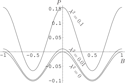
Figure 1: $P=C_{\tilde{t}}|\langle F_{S}\rangle|^{2}R\Lambda^{-3}/\pi$ and $B=\beta/(2\pi)$ for $\lambda^{2}=0$, 0.01, 0.1. The summation over $n$ appearing in (4.198) is taken as $\sum_{n=1}^{1000}$.

The eigenvalue equation (4.198) is invariant under the shift $B\to B^{\prime}=B+1$. For the shift, the left-hand side of (4.198) is explicitly written as

$${1\over\lambda^{2}-(B+1)^{2}}+\sum_{n=2}^{\infty}{1\over\lambda^{2}-(n+B)^{2}}+{1\over\lambda^{2}-B^{2}}+\sum_{n=1}^{\infty}{1\over\lambda^{2}-(n-B)^{2}},$$ (4.199)

which is the same as the original. From this point, invariance under the shift of $B$ with arbitrarily integer is induced. The eigenvalue equation (4.198) is also invariant under $B\leftrightarrow-B$. Thus we deal with values of the twist for $0\leq B\leq 1/2$. As seen in Figure 1, for $B=0$ (or $\beta=0$), a small eigenvalue is generated only for a small $P\propto\alpha$. In other words, then the eigenvalue and $P$ are the same order. When there is a nonzero Scherk-Schwarz twist, an interesting thing occurs. For $B\sim 0.5$, an eigenvalue $\lambda^{2}\sim 0.01$ is generated for $|P|\sim 0.1$ which is the same order as $B$. Even if $|P|$ and $B$ are the same order and not very small, a very small mass-eigenvalue can be generated due to the mixing of effects of $P$ and $B$. Taking the overall $R^{-2}$ back in Eq. (4.185), a TeV-scale mass splitting corresponds to $R^{-1}\sim 1~{}\textrm{TeV}$ for $\lambda\sim 1$ and $R^{-1}\gg\textrm{TeV}$ for $\lambda\ll 1$.

The appearance of small numbers with the mixing can be expected if we concentrate on the upper-left block matrix of Eq. (4.185). In the upper-left block matrix, if $P=0$, $B$ and the eigenvalue of the block matrix are the same order. If $B=0$, $P$ and the eigenvalue of the block matrix are the same order. Then a very small eigenvalue corresponds to the value itself of a very small $B$ or $P$. On the other hand, if $P$ and $B$ are both nonzero and a large mixing occurs, the eigenvalue can be much smaller than the values of $P$ and $B$.

Now we examine $\lambda$ as a function of $P$ for $B=1/2$. Using partial-fraction expansion of trigonometric functions

$$\pi\tan\pi\lambda=-{2\lambda\over\lambda^{2}-{1\over 4}}-\sum_{n=1}^{\infty}{2\lambda\over\lambda^{2}-\left(n+{1\over 2}\right)^{2}}=-\sum_{n=1}^{\infty}{2\lambda\over\lambda^{2}-\left(n-{1\over 2}\right)^{2}},$$ (4.200)

from Eq. (4.198) we obtain

$${\pi\tan\pi\lambda\over\lambda}=-{1\over P}.$$ (4.201)

The function $\lambda^{-1}\tan\pi\lambda$ has any value from $-\infty$ to $\infty$ for $n-{1\over 2}<\lambda<n+{1\over 2}$ for each $n$. Therefore, $\lambda$ in Eq. (4.201) has multiple solutions correspondingly to Kaluza-Klein modes. In Figure 2, behavior of each side of Eq. (4.201) against $\lambda$ is shown.

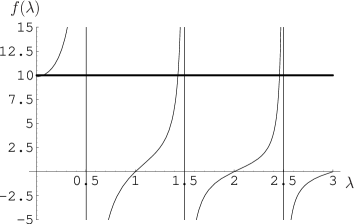
Figure 2: $f(\lambda)=\pi\lambda^{-1}\tan(\pi\lambda)$ (solid line) and $f(x)=-1/P$ (bold line). For illustration, the graph is shown for $P=-0.1$. In the right graph the neighborhood of the intersection for the lowest eigenvalue is magnified.

As seen in Figure 2, the mixing of $B$ and $|P|$ of order ${\cal O}(0.1)$ generates $\lambda$ of order ${\cal O}(0.01)$. A smaller lowest-eigenvalue can be generated by the mixing depending on the value of $P$. For a very small $\lambda$, with the expansion of $\tan(\pi\lambda)=(\pi\lambda)+(\pi\lambda)^{3}/3+\cdots$, Eq. (4.201) is

$$\pi^{2}+{\pi^{4}\lambda^{2}\over 3}+\cdots=-{1\over P},$$ (4.202)

up to ${\cal O}(\lambda^{4})$. To the order $\lambda^{2}$, the solution of the lowest-eigenvalue is obtained as

$$\lambda^{2}=-{3\over\pi^{4}}\left({1\over P}+\pi^{2}\right).$$ (4.203)

Because the left-hand side is positive, there is a lower bound to $P$,

$$P>-{1\over\pi^{2}}.$$ (4.204)

The existence of such a lower bound is seen in Figure 1.

In order to analyze the others of multiple solutions, we take the $n$-th eigenvalue (except for the lowest (4.203)) as $\lambda_{n}=n+{1\over 2}-\Delta_{n}$ to solve a small $\Delta_{n}$ perturbatively. The perturbation is valid especially for a large $n$ because $\Delta_{n}/n$ is very small for a large $n$. With this normalization, Eq. (4.201) is

$$\tan(\Delta_{n}\pi)=-{P\over n+\textrm{${1\over 2}$}-\Delta_{n}}.$$ (4.205)

By the expansion $\tan(\Delta_{n}\pi)=(\Delta_{n}\pi)+(\Delta_{n}\pi)^{3}/3+\cdots$, Eq. (4.205) is

$$\Delta_{n}^{2}-(n+\textrm{${1\over 2}$})\Delta_{n}-\textrm{${P\over\pi}$}=0,$$ (4.206)

up to ${\cal O}(\Delta_{n}^{3})$. We obtain the solution for $\Delta_{n}$,

$$\Delta_{n} \!\!\!=\!\!\! {1\over 2}\left[(n+\textrm{${1\over 2}$})\pm\sqrt{(n+\textrm{${1\over 2}$})^{2}+\textrm{${4P\over\pi}$}}\right]$$ (4.207)

$$\!\!\!=\!\!\! -{P\over(n+\textrm{${1\over 2}$})\pi}+{P^{2}\over(n+\textrm{${1\over 2}$})^{3}\pi^{2}}+\cdots,$$

where the ellipses denote higher order terms in the expansion with $P/(n+{1\over 2})^{2}$. The minus sign in the first line of Eq. (4.207) has been chosen so that the equation at the first-order of $\Delta_{n}$ is fulfilled.

Within the above approximation, we obtain the stop mass-eigenvalues squared

$$m_{\tilde{t}}^{2}=-{3\over R^{2}\pi^{4}}\left({1\over P}+\pi^{2}\right),~{}~{}{1\over R^{2}}\left(n+\textrm{${1\over 2}$}+{P\over(n+\textrm{${1\over 2}$})\pi}\right)^{2},$$ (4.208)

for $B=1/2$. For a generic $n$, the Kaluza-Klein mass is obtained as

$$m_{\tilde{t}}^{2}={1\over R^{2}}\left(n+\Delta\right)^{2},~{}~{}\Delta\approx 0.4-0.5.$$ (4.209)

as found in Figure 2.

The Higgs boson mass corrections

In Eq. (3.24) in Section 3, we wrote down the upper bound involving Kaluza-Klein modes. The analysis was based on the simplification that the $n$-th top and stop Kaluza-Klein masses are $n^{2}/R^{2}$ and ($m_{\tilde{t}}^{2}+n^{2}/R^{2}$), respectively. This structure of Kaluza-Klein masses are somehow different from the result given in Eqs. (4.208) and (4.209). We here derive the Higgs boson mass corrections for the lightest top and stop masses

$$m_{t}^{2}=|y_{t}|^{2}v_{2}^{2},\quad m_{\tilde{t}}^{2}=-{3\over R^{2}\pi^{4}}\left({1\over P}+\pi^{2}\right),$$ (4.210)

respectively and the $n$-th Kaluza-Klein top and stop masses

$$m_{t,n}^{2}={n^{2}\over R^{2}},\quad m_{\tilde{t},n}^{2}\approx{(n+\textrm{${1\over 2}$})^{2}\over R^{2}},$$ (4.211)

respectively. For the lightest top and stop with the masses (4.210), the correction to the Higgs boson mass is of the form (3.14),

$$\Delta_{t}={3\sqrt{2}m_{t}^{4}G_{F}\over 2\pi^{2}\sin^{2}\beta}\ln\left({m_{\tilde{t}}^{2}\over m_{t}^{2}}\right),$$ (4.212)

where $m_{t}$ and $m_{\tilde{t}}$ are given in Eq. (4.210). For the Kaluza-Klein mode, we adopt a calculation technique employed in Ref. [13] in which the potential

$$V={1\over 2}\textrm{Tr}\int{d^{4}p\over(2\pi)^{4}}\sum_{n=-\infty}^{\infty}\ln\left({p^{2}+M^{2}(\phi)+(n+q_{b})^{2}/R^{2}\over p^{2}+M^{2}(\phi)+(n+q_{f})^{2}/R^{2}}\right),$$ (4.213)

is led to

$$V \!\!\!=\!\!\! {1\over 128\pi^{6}R^{4}}\textrm{Tr}\left[V(q_{f},\phi)-V(q_{b},\phi)\right],$$ (4.214)

$$\!\!\!\!\!\!\!\!V(q,\phi) \!\!\!=\!\!\! (2\pi R)^{2}M^{2}(\phi)\textrm{Li}_{3}(e^{2i\pi q}e^{-2\pi R\sqrt{M^{2}(\phi)}})$$ (4.215)

$$+6\pi R\sqrt{M^{2}(\phi)}\textrm{Li}_{4}(e^{2i\pi q}e^{-2\pi R\sqrt{M^{2}(\phi)}})+3\textrm{Li}_{5}(e^{2i\pi q}e^{-2\pi R\sqrt{M^{2}(\phi)}})+\textrm{H.c.}.$$

where $\textrm{Li}_{n}(z)=\sum_{k=1}^{\infty}{z^{k}/k^{n}}$. While the zero-mode potential (3.9) is

$$U_{t}=6\int{d^{4}p\over(2\pi)^{4}}\ln\left({p^{2}+m_{\tilde{t}}^{2}+|y_{t}H_{2}^{0}|^{2}\over p^{2}+|y_{t}H_{2}^{0}|^{2}}\right),$$ (4.216)

with the stop mass (4.210), the potential contributed from Kaluza-Klein modes with the masses (4.211) can be written as

$$U_{t\,\textrm{\scriptsize KK}} \!\!\!=\!\!\! U_{\textrm{\scriptsize sum}}-U_{\textrm{\scriptsize sub}},$$ (4.217)

$$U_{\textrm{\scriptsize sum}} \!\!\!=\!\!\! 6\int{d^{4}p\over(2\pi)^{4}}\sum_{n=-\infty}^{\infty}\ln\left({p^{2}+|y_{t}H_{2}^{0}|^{2}+(n+\textrm{${1\over 2}$})^{2}/R^{2}\over p^{2}+|y_{t}H_{2}^{0}|^{2}+n^{2}/R^{2}}\right),$$ (4.218)

$$U_{\textrm{\scriptsize sub}} \!\!\!=\!\!\! 6\int{d^{4}p\over(2\pi)^{4}}\ln\left({p^{2}+|y_{t}H_{2}^{0}|^{2}+1/(4R^{2})\over p^{2}+|y_{t}H_{2}^{0}|^{2}}\right).$$ (4.219)

Using the formula

$$V(q_{b}=1/2,\phi) \!\!\!=\!\!\! -{(2\pi R)^{4}M^{4}(\phi)\over 4}\ln 2+\cdots,$$ (4.220)

$$V(q_{f}=0,\phi) \!\!\!=\!\!\! \left({3\over 16}-{1\over 4}\ln(2\pi R\sqrt{M^{2}(\phi)})\right)(2\pi R)^{4}M^{4}(\phi)+\cdots,$$ (4.221)

up to $M^{2}(\phi)$-linear term and higher order terms ${\cal O}((RM(\phi))^{5/2})$, we find the corrections for the Higgs boson mass,

$$\Delta_{\textrm{\scriptsize sum}}=2v_{2}^{2}U_{\textrm{\scriptsize sum}}^{\prime\prime}(v_{2}^{2}) \!\!\!=\!\!\! -{3\over 2\pi^{2}}{m_{t}^{4}\over v_{2}^{2}}\ln(\pi Rm_{t}),$$ (4.222)

$$\Delta_{\textrm{\scriptsize sub}}=2v_{2}^{2}U_{\textrm{\scriptsize sub}}^{\prime\prime}(v_{2}^{2}) \!\!\!=\!\!\! -{3\over 2\pi^{2}}{m_{t}^{4}\over v_{2}^{2}}\ln(2Rm_{t}).$$ (4.223)

Thus the Kaluza-Klein mode corrections are

$$\Delta_{t\,\textrm{\scriptsize KK}}=\Delta_{\textrm{\scriptsize sum}}-\Delta_{\textrm{\scriptsize sub}}={3\sqrt{2}m_{t}^{4}G_{F}\over\pi^{2}\sin^{2}\beta}\ln{2\over\pi}.$$ (4.224)

From this equation and the zero-mode contribution (4.212), we obtain the upper bound to the lightest Higgs boson mass,

$$m_{h^{0}}^{2}\leq m_{Z}\cos^{2}2\beta+{3\sqrt{2}m_{t}^{4}G_{F}\over 2\pi^{2}}\ln{(2m_{\tilde{t}})^{2}\over(\pi m_{t})^{2}},$$ (4.225)

with $m_{\tilde{t}}^{2}$ given in Eq. (4.210),

$$m_{\tilde{t}}^{2}=-{3\over R^{2}\pi^{4}}\left({1\over P}+\pi^{2}\right).$$ (4.226)

In Eq. (4.225), the Kaluza-Klein mode contribution is independent of $R$ and only $R$-dependence arises from the contribution of the lightest top and stop. The factor $\ln(m_{\tilde{t}}^{2}/m_{t}^{2})$ must not be too large for some $R$. For $B=1/2$, a large $R^{-1}$ can be allowed if $P^{-1}\sim-\pi^{2}$.

Here we estimate the values of radiative corrections. For $m_{t}=181~{}\textrm{GeV}$ and $m_{\tilde{t}}\sim 1000~{}\textrm{GeV}$ (composed of various values of $R$ and $P$ via Eq. (4.226)), the lightest mode contribution gives

$${3\sqrt{2}m_{t}^{4}G_{F}\over 2\pi^{2}}\ln\left({m_{\tilde{t}}^{2}\over m_{t}^{2}}\right)\approx(96\textrm{GeV})^{2}.$$ (4.227)

On the other hand, the Kaluza-Klein contribution makes

$${3\sqrt{2}m_{t}^{4}G_{F}\over 2\pi^{2}}\ln{4\over\pi^{2}}\approx-(50~{}\textrm{GeV})^{2}.$$ (4.228)

Such a negative Kaluza-Klein contribution can be generated because in Eq. (4.218) the argument of the logarithm function is smaller than unity for $n<0$. These contributions $(96\textrm{GeV})^{2}-(50\textrm{GeV})^{2}=(82\textrm{GeV})^{2}$ can change the upper bound to the mass of the lightest Higgs boson into an allowed region.

In the present model, gauge bosons propagate in bulk. The gauge coupling is sensitive to energies over the inverse compactification scale [37]-[46]. As a fundamental theory appears before gauge couplings become very small or very large, the number of Kaluza-Klein modes can be of at most ${\cal O}(100)$. Thus an ultraviolet momentum cutoff may be introduced in the theory. Our result for the radiative correction to the Higgs boson mass is independent of such a cutoff.

5 Conclusion

We have studied corrections to the mass of the lightest Higgs boson in a Kaluza-Klein effective theory. For the simple spectrum, it has been explicitly shown how contributions of Kaluza-Klein modes to the Higgs boson mass correction are summed. There the summation over infinite numbers of Kaluza-Klein mode contributions converges. In other cases, a finite radiative correction has been obtained using a calculation technique employed in the context with the summation over zero mode and Kaluza-Klein modes and a momentum integral.

While $N=1$ supersymmetry is oriented differently on each brane depending on a Scherk-Schwarz twist, an $F$-term on a brane has been introduced. For these two sources, stop mass matrix is non-diagonal with respect to Kaluza-Klein modes and also with respect to SU(2)_R. We have pointed out that a very small eigenvalue can be accommodated in the diagonalized basis. Thus the mass splitting between zero-mode stop and top can be around $1~{}$TeV even for a large $R^{-1}$. A large inverse compactification scale may be motivated by four-dimensional MSSM gauge coupling unification. It has also been shown that the eigenvalue equation becomes a simple form with trigonometric functions for the Scherk-Schwarz parameter $\beta=\pi$. In this case we have presented multiple solutions that correspond to Kaluza-Klein modes. With these solutions, we have estimated radiative corrections to the lightest Higgs boson mass.

In the context of extra dimensions, the mass splitting may be related to the inverse scale of compactification. The stop mass can be

$$m_{\tilde{t}}\sim c\times{1\over R},$$ (5.1)

where $c$ is a numerical factor. On the other hand, Kaluza-Klein masses are proportional to $R^{-1}$. From these properties, the correction of Kaluza-Klein modes to the lightest Higgs boson mass squared is independent of $R$ as in Eqs. (3.21) and (4.224). This Kaluza-Klein contribution can be around over $3m_{t}^{4}G_{F}/(\sqrt{2}\pi^{2})=(52~{}\textrm{GeV})^{2}$. Together with zero-mode contribution, it lifts the upper bound to the lightest Higgs boson in an allowed region, although the value of zero mode contribution depends on $R$.

Finally, we mention stabilization of the scale $R$. A simple setup to stabilize compactification radius is to take a constant superpotential into account in a warped extra dimension [19, 49, 50]. It may be interesting to examine the issue of the Higgs boson mass for the mixing of two supersymmetry breaking sources in a warped model with radius stabilization.

Acknowledgments

I am grateful to Masud Chaichian for a careful reading of the manuscript.

References

- [1] Stephen P. Martin, arXiv:hep-ph/9709356.
- [2] E. A. Mirabelli and M. E. Peskin, Phys. Rev. D 58, 065002 (1998) [arXiv:hep-th/9712214].
- [3] L. Randall and R. Sundrum, Nucl. Phys. B 557, 79 (1999) [arXiv:hep-th/9810155].
- [4] D. E. Kaplan, G. D. Kribs and M. Schmaltz, Phys. Rev. D 62, 035010 (2000) [arXiv:hep-ph/9911293].
- [5] Z. Chacko, M. A. Luty, A. E. Nelson and E. Ponton, JHEP 0001, 003 (2000) [arXiv:hep-ph/9911323].
- [6] D. Marti and A. Pomarol, Phys. Rev. D 64, 105025 (2001) [arXiv:hep-th/0106256].
- [7] V. Di Clemente, S. F. King and D. A. J. Rayner, Nucl. Phys. B 617, 71 (2001) [arXiv:hep-ph/0107290].
- [8] V. Di Clemente, S. F. King and D. A. J. Rayner, Nucl. Phys. B 646, 24 (2002) [arXiv:hep-ph/0205010].
- [9] J. Scherk and J. H. Schwarz, Phys. Lett. B 82, 60 (1979).
- [10] J. Scherk and J. H. Schwarz, Nucl. Phys. B 153, 61 (1979).
- [11] I. Antoniadis, Phys. Lett. B 246, 377 (1990).
- [12] A. Pomarol and M. Quiros, Phys. Lett. B 438, 255 (1998) [arXiv:hep-ph/9806263].
- [13] A. Delgado, A. Pomarol and M. Quiros, Phys. Rev. D 60, 095008 (1999) [arXiv:hep-ph/9812489].
- [14] R. Barbieri, L. J. Hall and Y. Nomura, Nucl. Phys. B 624, 63 (2002) [arXiv:hep-th/0107004].
- [15] J. A. Bagger, F. Feruglio and F. Zwirner, Phys. Rev. Lett. 88, 101601 (2002) [arXiv:hep-th/0107128].
- [16] J. Bagger, F. Feruglio and F. Zwirner, JHEP 0202, 010 (2002) [arXiv:hep-th/0108010].
- [17] C. Biggio, F. Feruglio, A. Wulzer and F. Zwirner, JHEP 0211, 013 (2002) [arXiv:hep-th/0209046].
- [18] N. Haba, Y. Hosotani and Y. Kawamura, Prog. Theor. Phys. 111, 265 (2004) [arXiv:hep-ph/0309088].
- [19] N. Maru, N. Sakai and N. Uekusa, Phys. Rev. D 74, 045017 (2006) [arXiv:hep-th/0602123].
- [20] D. Diego, G. von Gersdorff and M. Quiros, Phys. Rev. D 74, 055004 (2006) [arXiv:hep-ph/0605024].
- [21] H. Hatanaka, T. Inami and C. S. Lim, Mod. Phys. Lett. A 13, 2601 (1998) [arXiv:hep-th/9805067].
- [22] I. Antoniadis, K. Benakli and M. Quiros, Nucl. Phys. B 583, 35 (2000) [arXiv:hep-ph/0004091].
- [23] A. Delgado and M. Quiros, Phys. Lett. B 484, 355 (2000) [arXiv:hep-ph/0004124].
- [24] R. Barbieri, L. J. Hall and Y. Nomura, Phys. Rev. D 63, 105007 (2001) [arXiv:hep-ph/0011311].
- [25] N. Arkani-Hamed, L. J. Hall, Y. Nomura, D. Tucker-Smith and N. Weiner, Nucl. Phys. B 605, 81 (2001) [arXiv:hep-ph/0102090].
- [26] A. Delgado and M. Quiros, Nucl. Phys. B 607, 99 (2001) [arXiv:hep-ph/0103058].
- [27] D. M. Ghilencea and H. P. Nilles, Phys. Lett. B 507, 327 (2001) [arXiv:hep-ph/0103151].
- [28] A. Delgado, G. von Gersdorff and M. Quiros, Nucl. Phys. B 613, 49 (2001) [arXiv:hep-ph/0107233].
- [29] V. Di Clemente and Y. A. Kubyshin, Nucl. Phys. B 636, 115 (2002) [arXiv:hep-th/0108117].
- [30] D. M. Ghilencea, H. P. Nilles and S. Stieberger, New J. Phys. 4, 15 (2002) [arXiv:hep-th/0108183].
- [31] D. M. Ghilencea, S. Groot Nibbelink and H. P. Nilles, Nucl. Phys. B 619, 385 (2001) [arXiv:hep-th/0108184].
- [32] D. M. Ghilencea, JHEP 0503, 009 (2005) [arXiv:hep-ph/0409214].
- [33] D. M. Ghilencea and H. M. Lee, JHEP 0509, 024 (2005) [arXiv:hep-ph/0505187].
- [34] G. Bhattacharyya, S. K. Majee and A. Raychaudhuri, Nucl. Phys. B 793, 114 (2008) [arXiv:0705.3103 [hep-ph]].
- [35] C. S. Lim and N. Maru, Phys. Lett. B 653, 320 (2007) [arXiv:0706.1397 [hep-ph]].
- [36] S. Weinberg, The Quantum Theory of Fields, Volume III Supersymmetry, Cambridge University Press, 2005, section 28.5.
- [37] K. R. Dienes, E. Dudas and T. Gherghetta, Phys. Lett. B 436, 55 (1998) [arXiv:hep-ph/9803466].
- [38] K. R. Dienes, E. Dudas and T. Gherghetta, Nucl. Phys. B 537, 47 (1999) [arXiv:hep-ph/9806292].
- [39] L. J. Hall and Y. Nomura, Phys. Rev. D 64, 055003 (2001) [arXiv:hep-ph/0103125].
- [40] Y. Nomura, D. R. Smith and N. Weiner, Nucl. Phys. B 613, 147 (2001) [arXiv:hep-ph/0104041].
- [41] A. Hebecker and J. March-Russell, Nucl. Phys. B 613, 3 (2001) [arXiv:hep-ph/0106166].
- [42] R. Contino, L. Pilo, R. Rattazzi and E. Trincherini, Nucl. Phys. B 622, 227 (2002) [arXiv:hep-ph/0108102].
- [43] G. Bhattacharyya, A. Datta, S. K. Majee and A. Raychaudhuri, Nucl. Phys. B 760, 117 (2007) [arXiv:hep-ph/0608208].
- [44] N. Arkani-Hamed, D. E. Kaplan, H. Murayama and Y. Nomura, JHEP 0102, 041 (2001) [arXiv:hep-ph/0012103].
- [45] N. Uekusa, Phys. Rev. D 75, 064014 (2007) [arXiv:hep-th/0701159].
- [46] N. Uekusa, arXiv:0803.1537 [hep-ph].
- [47] N. Arkani-Hamed, T. Gregoire and J. G. Wacker, JHEP 0203, 055 (2002) [arXiv:hep-th/0101233].
- [48] A. Hebecker, Nucl. Phys. B 632, 101 (2002) [arXiv:hep-ph/0112230].
- [49] N. Maru, N. Sakai and N. Uekusa, Phys. Rev. D 75, 125014 (2007) [arXiv:hep-th/0612071].
- [50] N. Uekusa, Mod. Phys. Lett. A 23, 603 (2008) [arXiv:0704.2490 [hep-th]].