Fractional derivatives of random walks: Time series with long-time memory

Abstract

We review statistical properties of models generated by the application of a (positive and negative order) fractional derivative operator to a standard random walk and show that the resulting stochastic walks display slowly-decaying autocorrelation functions. The relation between these correlated walks and the well-known fractionally integrated autoregressive (FIGARCH) models, commonly used in econometric studies, is discussed. The application of correlated random walks to simulate empirical financial times series is considered and compared with the predictions from FIGARCH and the simpler FIARCH processes. A comparison with empirical data is performed.

I Introduction

In recent years, there has been a surging interest in the application of non-integer order differential operators to describe different types of temporal and spatial anomalies displayed by complex systems GionaRoman:1992 ; FracFokkerPlanck:1998 ; OldhamSpanier:1974 ; Podlubny:1999 ; Metzler:2000 ; Hilfer:2000 ; Gorenflo:2002 ; Gorenflo:2007 ; Scherer:2007 . For example, a fractional diffusion equation suitably describes the asymptotic behavior of independent random walkers on random fractal structures GionaRoman:1992 , and also corresponding fractional Fokker-Planck equations have been used to model anomalous behavior FracFokkerPlanck:1998 . Several recent reviews can be found in literature covering a vast field of applications (see e.g. Metzler:2000 ; Hilfer:2000 ). A treatment from a mathematical point of view can be found in OldhamSpanier:1974 ; Podlubny:1999 . Closely related to the present work is the subject of fractional derivative operators as discussed within the framework of random walks Gorenflo:2002 ; Gorenflo:2007 and anomalous transport phenomena Scherer:2007 .

Random walks play also an essential role in modeling the time evolution of stock prices. The literature in the field is huge and we just mention few papers related with the present work onefactormodel ; Gopikrishnan1998 ; Borland:1998 ; MantegnaStanley ; Bouchaud:2001 ; Podobnik2006 ; Roman2006 ; Scalas:2006 ; McCauley:2007 . The different features studied include stock-index cross-correlations onefactormodel , probability distribution functions of log-returns Gopikrishnan1998 ; Borland:1998 ; MantegnaStanley ; Bouchaud:2001 ; Podobnik2006 ; Roman2006 ; Scalas:2006 ; McCauley:2007 , leverage effect Bouchaud:2001 , stock-stock cross-correlations and market internal structure Roman2006 , tick-by-tick behavior Scalas:2006 , non-stationarity issues McCauley:2007 .

A succesful and widely used model to describe price variations is based on an autoregressive process with conditional heteroskedasticity (ARCH) due to Engle (see e.g. arch ), of which simple variants have been recently suggested RomanPorto2001 ; DosePortoRoman2003 . Further variants of ARCH models have been recently discussed with regards to volatility tarch ; tarch:Palatella2004 . ARCH type models have been generalized to incorporate a long-time memory in the surrogate time series, in an attempt to mimick the strong autocorrelations observed in volatility and absolute returns Granger1980 ; Bollerslev:1986 ; Engle/Bollerslev:1986 ; Baillie1996 ; Zumbach2004 ; Tang2006 .

The issue of long-time autocorrelations, or long time memory, in time series is intimately related with the concept of Hurst exponent, introduced by Hurst many years ago to describe the persistence observed in the behavior of Nile floods Hurst:1951 . Motivated by these ideas, Mandelbrot introduced few years later a long-time memory model known as fractional Brownian motion (FBM), being stationary on all time scales, as an attempt to model such anomalous phenomena Mandelbrot:1968 . Rigorous mathematical aspects of FBM can be found in textbooks fBm:math , the latter including also a discussion of Lévy processes with long-time memory. A recent work considers other aspects of the FBM model Perez2006-fBm .

The problem of accurately determining the Hurst exponent of a time series has been the subject of intense activity, started with the description of persistence in DNA sequences in which the detrended fluctuation analysis (DFA) has been introduced Peng:1994 . Further developments were achieved based on Haar wavelets Kantelhardt:1995 and its generalization to higher orders PRL1998 . In the present work, we will make use of Haar wavelet techniques to analyse the surrogate time series and determining the associated Hurst exponents.

In this work, we apply a fractional derivation (and integration) operator to an uncorrelated random walk, obtained within a simple ARCH prescription, to generate a surrogate financial time series with uncorrelated variations on all time lags, but having a slowly decaying auto-correlation for the absolute variations, representing the absolute returns. The new process is denoted as fractional random walk ARCH (FRWARCH) and we show that it has finite second moments, in contrast to FIGARCH processes characterized by an infinite variance. We will conclude that FRWARCH can become a useful tool in econometrics applications.

The paper is organized as follows. In Sect. II, we briefly review the fractional derivative operator and its main properties. In Sect. III, we discuss the effects of applying a fractional derivative (and fractional integration) operator to a standard random walk. The scaling properties of the resulting fractional random walk are discussed. Sect. IV is devoted to FRWARCH, for which the associated probability distribution functions and auto-correlations are studied. In Sect. V, we review the widely used FIGARCH process and discuss several of its properties in comparison with those of FRWARCH. In Sect. VI we briefly consider, for completeness, the simpler fractionally integrated ARCH models currently used in literature. In Sect. VII we present a brief comparison of FRWARCH and FIGARCH with empirical data to see how they actually perform in more realistic situations. Reference is made to a simpler generalized ARCH model without long-range memory, but having a slow decaying autocorrelation function, to better understand the role of memory in the models presented here. Finally, Sect. VIII summarizes the main conclusions of the work.

II Fractional derivative operator

Let us consider a time-dependent function $y(t)$ recorded at times $t=i\tau$, where $0\leq i\leq N$ and $\tau$ is the time resolution. For simplicity, we will indicate the associated time series as $y_{i}$.

In the following, we study the fractional derivative (finite difference) operator of fractional order $\alpha$, $D_{\tau}^{(\alpha)}$, known in literature as the Grünwald-Letnikov scheme (see e.g. Gorenflo:2002 ; Scherer:2007 ), which is defined as

$$D_{\tau}^{(\alpha)}y_{n}={1\over\tau^{\alpha}}\sum_{i=0}^{n}(-1)^{i}{\alpha\choose i}y_{n-i}$$ (1)

where

$${\alpha\choose i}={\Gamma(\alpha+1)\over\Gamma(i+1)\Gamma(\alpha+1-i)}$$ (2)

is the binomial coefficient and $\Gamma(x)$ is the Gamma function Abramowitz:1972 .

For the numerical implementation of Eq. (1), it is more convenient to work out an equivalent expression for the binomial coefficients in Eq. (2). This will also allow us to make contact with long-range memory models known from the financial literature. Using the properties of the $\Gamma(x)$ function Abramowitz:1972 , one can show that

$${\alpha\choose i}={\alpha(\alpha-1)(\alpha-2)...(\alpha-i+1)\over i!},$$ (3)

where the numerator is a polynomial of $i$th degree in $\alpha$. Using Eq. (3), Eq. (1) becomes

$$D_{\tau}^{(\alpha)}y_{n} = {1\over\tau^{\alpha}}\left[~{}y_{n}\right.-\alpha y_{n-1}+{\alpha\over 2!}(\alpha-1)y_{n-2}-\dots$$ (4)

$$+ (-1)^{n}{\alpha\over n!}(\alpha-1)\dots(\alpha-n+1)y_{0}\left.\right].$$

In what follows, we will consider values of $\alpha$ in the range $-1<\alpha<1$. Indeed, it is easy to see from Eq. (4) that the case $\alpha=1$ corresponds to the (Euler) first order derivative of $y_{n}$, i.e.,

$$D_{\tau}^{(1)}y_{n}={1\over\tau}(y_{n}-y_{n-1}),$$ (5)

while the value $\alpha=-1$ yields the integral of $y_{n}$,

$$D_{\tau}^{(-1)}y_{n}=\tau(y_{n}+y_{n-1}+y_{n-2}+\dots+y_{0})=\sum_{i=0}^{n}y_{i}\tau.$$ (6)

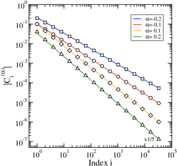
Figure 1: (color online) The absolute value of the coefficients $|C_{i}^{(\alpha)}|$ vs index $i$, for different values of the fractional order $\alpha=-0.2$ (squares), -0.1 (circles), 0.1 (diamonds) and 0.2 (triangles). The symbols represent the numerically evaluated coefficients using Eq. (3) and the straight lines the asymptotic result, Eq. (9). The results for $\alpha=0.2$ have been multiplied (down shifted) by a factor 1/5 for clarity.

It is also instructive to derive the asymptotic behavior of the coefficients in the expansion of the fractional operator. To do this, we write Eq. (3) in the form

$${\alpha\choose i}=(-1)^{i}{(0-\alpha)(1-\alpha)(2-\alpha)...(i-1-\alpha)\over i!}.$$ (7)

Now, using the relation $\prod_{j=0}^{i-1}(j+z)=\Gamma(i+z)/\Gamma(z)$ Abramowitz:1972 in Eq. (7), with $z=-\alpha$, the coefficient $C_{i}^{(\alpha)}\equiv(-1)^{i}{\alpha\choose i}$ can be written as

$$C_{i}^{(\alpha)} = {\Gamma(i+z)\over\Gamma(z)~{}i!}$$ (8)

$$= {\Gamma(i-\alpha)\over\Gamma(-\alpha)\Gamma(i+1)}=-{\alpha\over\Gamma(1-\alpha)}{\Gamma(i-\alpha)\over\Gamma(i+1)},$$

where the known relations $\Gamma(1+z)=z\Gamma(z)$ and $i!=\Gamma(i+1)$ have been used. Exploiting the large argument expansion $\Gamma(az+b)\simeq\exp(-az)(az)^{az+b-1/2}$, one can obtain the asymptotic behavior of $C_{i}^{(\alpha)}$ for large $i$ as

$$C_{i}^{(\alpha)}\simeq-{\alpha\over\Gamma(1-\alpha)}i^{-(1+\alpha)},\qquad i\gg 1,$$ (9)

which is positive for $\alpha<0$ and negative for $\alpha>0$. Results for $|C_{i}^{(\alpha)}|$ are plotted in Fig. 1 in double logarithmic scale for few representative values of $\alpha$. To be noted is the rather quick approach of the actual value of $C_{i}^{(\alpha)}$ to its asymptotic form Eq. (9). This feature can be used in numerical calculations where $C_{i}^{(\alpha)}$ can be replaced by Eq. (9) when the difference between the two is sufficiently small.

It is natural to refer to $D_{\tau}^{(\alpha)}$ as a fractional derivative operator for values $0<\alpha<1$ and as a fractional integral operator when $-1<\alpha<0$. This can be seen in the case that $y_{n}\simeq n^{\gamma}$. In fact, the action of the fractional operator, which will be denoted as

$$D_{\tau}^{(\alpha)}y_{n}\equiv y_{n}^{(\alpha)}={1\over\tau^{\alpha}}\sum_{i=0}^{n}C_{i}^{(\alpha)}y_{n-i},$$ (10)

can be estimated for large $n$ using the asymptotic behavior for $C_{i}^{(\alpha)}$, Eq. (9). Roughly, we can write $y_{n}^{(\alpha)}\simeq\int_{1}^{n}dx~{}x^{-(1+\alpha)}~{}(n-x)^{\gamma}$. When $\gamma\geq 0$ and $n\gg 1$, the largest contribution to the integral comes from the smallest values of $x$, yielding $y_{n}^{(\alpha)}\sim~{}n^{\gamma}\int_{1}^{n}dx~{}x^{-(1+\alpha)}\sim n^{\gamma-\alpha}$. Thus,

$$D_{\tau}^{(\alpha)}y_{n}\simeq n^{\gamma-\alpha}.$$ (11)

We show in Fig. 2 numerical examples of the fractional operation $D_{1}^{(\alpha)}y_{n}$ (i.e. $\tau=1$) in the case $y_{n}=1$ ($\gamma=0$), as an illustration of the result Eq. (11). Note that for a constant function $y_{n}$, the slope of the curves is just minus the order of the fractional operator. To be noted also is the rather quick approach of the fractional operator result Eq. (10) to its asymptotic behavior Eq. (11), already for small values of $n$.

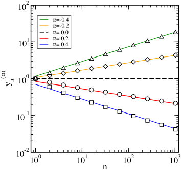
Figure 2: (color online) The fractional function $y_{n}^{(\alpha)}=D_{\tau}^{(\alpha)}y_{n}$ vs index $n$, in the case $y_{n}=1$ (i.e. $\gamma=0$), $\tau=1$, for different values of the fractional order: $\alpha=0.4$ (squares), 0.2 (circles), -0.2 (diamonds) and -0.4 (triangles). The symbols represent the numerical results using Eq. (4), and the straight lines the asymptotic form, Eq. (11). The dashed line corresponds to the original series $y_{n}$.

III Fractional random walks

Let us consider the case in which $y_{n}$ represents a standard random walk (RW), and assume the time resolution $\tau=1$ for convenience. Specifically, $y_{n}$ is constructed as a sum of independent, equally distributed random numbers, $\eta$. Without loss of generality, let us assume the latter are drawn from a Gaussian distribution of zero mean and unit standard deviation, i.e. $\big{<}\eta\big{>}=0$ and $\big{<}\eta^{2}\big{>}=1$, yielding $\sigma_{\eta}=1$. Thus,

$$y_{n}=\sum_{i=1}^{n}\eta_{i},\qquad 1\leq n\leq N,$$ (12)

where we take $y_{0}=0$ for simplicity. We are interested in studying the behavior of the associated fractional random walks (FRW’s), obtained by applying the fractional operator $D_{1}^{(\alpha)}$ to the random walk ‘profile’ $y_{n}$, Eq. (12), $D_{1}^{(\alpha)}y_{n}=y_{n}^{(\alpha)}$.

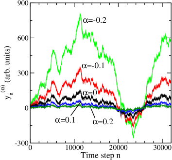
Figure 3: (color online) Fractional random walks: Plots of $y_{n}^{(\alpha)}$ versus time step $n$, for selected values of $\alpha$ as indicated on the plot. The standard RW corresponding to $\alpha=0$, $y_{n}^{(0)}\equiv y_{n}$, is also shown for comparison. The walks consist of $N=32000$ steps each.

Examples of fractional walks $y_{n}^{(\alpha)}$ are illustrated in Fig. 3. As is apparent from the figure, the amplitude of the fractional walks increases for negative $\alpha$ with respect to the uncorrelated case $y_{n}$, while for positive $\alpha$ the amplitude of the walks gets smaller. The question is whether the fractional walks are also statistically different from the uncorrelated case in the sense that long-range autocorrelations are present. Before discussing this quest, let us consider next the distribution function of the increments of a FRW.

III.1 Probability distribution functions

The increments of a fractional random walk are denoted as

$$\Delta y_{n}^{(\alpha)}=y_{n}^{(\alpha)}-y_{n-1}^{(\alpha)}.$$ (13)

For a standard random walk, as in Eq. (12), one simply has $\Delta y_{n}=\eta_{n}$, which is a local function of the time step $n$, i.e. independent of the previous values of $\eta_{i}$, $i<n$. In contrast, for any fractional order $\alpha$ ($\neq 0$), we find

$$\Delta y_{n}^{(\alpha)} = \sum_{i=0}^{n}C_{i}^{(\alpha)}y_{n-i}-\sum_{i=0}^{n-1}C_{i}^{(\alpha)}y_{n-1-i}$$ (14)

$$= C_{n}^{(\alpha)}y_{0}+\sum_{i=0}^{n-1}C_{i}^{(\alpha)}(y_{n-i}-y_{n-1-i})$$

$$= \sum_{i=0}^{n-1}C_{i}^{(\alpha)}\eta_{n-i},$$

where we have taken $y_{0}=0$. Thus, for fractional $\alpha$, the increments of the fractional random walk, $\Delta y_{n}^{(\alpha)}$, require the knowledge of the whole history of the walk, $\{\eta_{i}\}$, with $1\leq i\leq n$. This result suggests that FRW’s may possess long-range autocorrelations, as we will indeed see below.

The probability distribution function (PDF) of the increments, denoted as $G(g)$, is a function of the scaled variable $g\equiv g_{n}=(\Delta y_{n}^{(\alpha)}-\big{<}\Delta y_{n}^{(\alpha)}\big{>})/\sigma_{\alpha}$, where $\sigma_{\alpha}$ is the standard deviation of $\Delta y_{n}^{(\alpha)}$. If $\eta$ is normally distributed, $G(\eta)=G_{0}(\eta)=(2\pi)^{-1/2}\exp(-\eta^{2}/2)$, so is also $G(g)$. This does not hold in general for distributions $G(\eta)\neq G_{0}(\eta)$ because the coefficients $C_{i}^{(\alpha)}$ in Eq. (14), weighting the $\eta_{n-i}$’s differently, can yield effectively non-indentically distributed random numbers and the central limit theorem does not hold. To see this in a simple case, consider that $C_{i}^{(\alpha)}=\exp(-i/\alpha)$. Now, if $\alpha\to 0$ then $G(g)=G(\eta)$. Also for finite $\alpha\ll 1$, the distribution $G(g)$ will not be Gaussian. In the present case, we illustrate this behavior by assuming that $G(\eta)=\exp(-|\eta|)$. The corresponding PDF’s for $g$ are shown in Fig. 4 in the case $\alpha=-0.2$ for series of different length $N$, where $0\leq n\leq N$. As one can see from the figure, $G(g)$ remains exponentially distributed attaining the form $G(g)\simeq A\exp(-|g|/A)$, with $A\simeq 0.7$.

Figure 4: (color online) PDF, $G(g)$, for fractional random walks variations $\Delta y_{n}^{(\alpha)}$ as a function of the scaled variable $g=(\Delta y_{n}^{(\alpha)}-\big{<}\Delta y_{n}^{(\alpha)}\big{>})/\sigma_{\alpha}$ in the case $\alpha=-0.2$ (see Fig. 3), for series of different length $N$ ($0\leq n\leq N$) indicated in the inset. The continuous line is the normal distribution, while the dashed line is the exponential form $f(g)=A_{1}\exp(-|g|/A2)$, with $A_{1}=0.72$ and $A_{2}=0.7$.

III.2 Auto-correlations

Since for a standard RW the profile behaves, in a statistical sense, as $y_{n}\sim n^{1/2}$, actually meaning that $\big{<}(y_{n}-y_{n+m})^{2}\big{>}\sim|m|$, the fractional random walk obeys

$$y_{n}^{(\alpha)}\simeq n^{1/2-\alpha},$$ (15)

corresponding to $\big{<}(y_{n}^{(\alpha)}-y_{n+m}^{(\alpha)})^{2}\big{>}\sim|m|^{1-2\alpha}$. Identifying in Eq. (15) the power of $n$ with the Hurst exponent $H$ Hurst:1951 we find,

$$H={1\over 2}-\alpha,\qquad{\rm and}\qquad\alpha={1\over 2}-H.$$ (16)

Here, we are interested in cases where $0<H<1$, yielding for $\alpha$ the range of variation $-1/2<\alpha<1/2$. The case $H=1/2$ corresponds to standard (uncorrelated) behavior, values $H>1/2$ indicate persistence or long-time autocorrelations, while values $H<1/2$ yield anti-persistence or negative autocorrelations.

The Hurst exponent also determines the behavior of the auto-correlation function of the increments $\Delta y_{n}^{(\alpha)}$, $\mathcal{C}_{\alpha}(m)$, which is given by $\mathcal{C}_{\alpha}(m)=\big{<}g_{n}g_{n+m}\big{>}$. If long-range memory is indeed present, the autocorrelation function is expected to obey the scaling behavior $\mathcal{C}_{\alpha}(m)\sim|m|^{-2(1-H)}$ (see e.g. Peng:1994 ; PRL1998 ), yielding

$$\mathcal{C}_{\alpha}(m)\simeq-{\rm sign}(\alpha)~{}|m|^{-(1+2\alpha)},\qquad|m|\gg 1.$$ (17)

To detect the presence of long-range memory for a fractional random walk $y_{n}^{(\alpha)}$, we apply the method known in literature as the fluctuation analysis (FA) PRL1998 based on Haar wavelets (HW) Kantelhardt:1995 , consisting in studying the scaling behavior of $y_{n}^{(\alpha)}$ on the time scale $t$. To do this, the total number of points in the series, $N$, is divided into consecutive non-overlaping segments of length $\ell\geq 1$, corresponding to the time scale $t=\ell\tau$. Inside each segment $s$, $1\leq s\leq N/\ell$, the average of $y_{n}^{(\alpha)}$, denoted as $B_{s}(\ell)$, is evaluated according to

$$B_{s}(\ell)=\frac{1}{\ell}\sum_{j=1}^{\ell}y^{(\alpha)}_{(s-1)\ell+j}.$$ (18)

The FAHW approach consists in studying the fluctuations of the profile on the time scale $\ell=t/\tau$, defined as

$$F(\ell)=\big{<}\big{[}B_{s}(\ell)-B_{s-1}(\ell)\big{]}^{2}\big{>}^{1/2},$$ (19)

corresponding to the first-order Haar wavelet, and the average is performed over all consecutive boxes $s$ and $s-1$. To be noted is that Eq. (19) can be generalized to higher order wavelets PRL1998 .

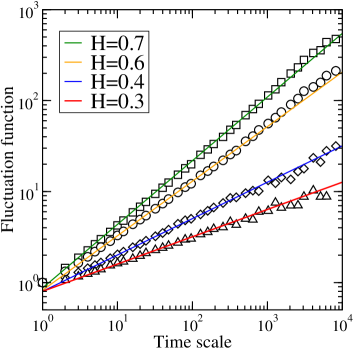
Figure 5: (color online) Fluctuation analysis of fractional random walks: Plotted is the fluctuation function $F(\ell)/F(1)$ vs time scale $\ell$ for different values of fractional order: $\alpha=0.2$ (triangles), 0.1 (diamonds), -0.1 (circles) and -0.2 (squares). The straight lines have slopes $H=1/2-\alpha$ given by Eq. (16). The series considered consist of $N=10^{5}$ time steps each.

The dependence of $F(\ell)$ on $\ell$ is expected to obey a scaling behavior of the form

$$F(\ell)\sim\ell^{H},$$ (20)

from which one can obtain the Hurst exponent $H$. Results for the fractional orders considered in Fig. 3 are reported in Fig. 5. The results support the expectations of the existence of long-range memory for FRW’s.

IV Fractional random walks for financial time series

It is well known that daily log-returns, i.e. the variation of the logarithm of asset price $P_{n}$ at day $n$, denoted as $\Delta S_{n}=\ln P_{n}-\ln P_{n-1}$, is not correlated with its variations $\Delta S_{n^{\prime}\neq n}$ and the corresponding PDF displays power-law tails, $G(g)\sim|g|^{-\beta}$ with $\beta\approx 4$ (see e.g. Gopikrishnan1998 ; Roman2006 ). In addition, absolute log-returns, that is $|\Delta S_{n}|$, appear to be long-range auto-correlated (see e.g. MantegnaStanley ; FBMRomanPortoPrepr ). We aim at modeling these features using the FRW described above for negative values of $\alpha$.

In order to obtain a PDF for log-returns displaying power-law tails, we resort to a simple auto-regressive conditional heteroskedastic model (ARCH) arch . We define the log-returns according to

$$\Delta S_{n}=\sigma_{n}\eta_{n},\qquad n\geq 1,$$ (21)

where $\eta_{n}$ are uncorrelated random numbers drawn from a normal distribution with zero mean and unit variance, i.e. $\big{<}\eta_{n}^{2}\big{>}=1$ and $\big{<}\Delta S_{n}\Delta S_{m}\big{>}=\big{<}(\Delta S)^{2}\big{>}\delta_{n,m}$. The standard deviation $\sigma_{n}$ changes in time according to the ARCH prescription,

$$\sigma_{n}^{2}=a+b~{}(\Delta X_{n-1}^{(\alpha)})^{2},$$ (22)

where $\Delta X_{n-1}^{(\alpha)}$ is proportional to the fractional integral of $\Delta S_{n-1}$, Eq. (10),

$$\Delta X_{n-1}^{(\alpha)}={1\over A_{n-1}(\alpha)}D_{1}^{(\alpha)}\Delta S_{n-1},\qquad\alpha<0,$$ (23)

and the factor $A_{n-1}(\alpha)=\sqrt{\sum_{i=0}^{n-1}(C_{i}^{(\alpha)})^{2}}$ ensures the constancy of the 2nd moment $\big{<}(\Delta X_{n-1}^{(\alpha)})^{2}\big{>}$. Indeed, using Eq. (10) the latter becomes

$$\big{<}(\Delta X_{n-1}^{(\alpha)})^{2}\big{>} = {1\over A^{2}_{n-1}(\alpha)}\sum_{i=0}^{n-1}\left(C_{i}^{(\alpha)}\right)^{2}\big{<}\big{(}\Delta S_{n-1-i}\big{)}^{2}\big{>},$$ (24)

$$\equiv \big{<}\big{(}\Delta S\big{)}^{2}\big{>}=\sigma_{\rm A}^{2},$$

where we find $\sigma_{\rm A}^{2}=a/(1-b)$ according to Eq. (22). Plots of $A_{n}(\alpha)$ are shown in Fig. 6. The present combination of a FRW with ARCH will be denoted for brevity FRWARCH.

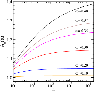
Figure 6: (color online) The normalization coefficients $A_{n}(\alpha)$ versus $n$ for different values of $\alpha$ (from top to bottom): $\alpha=-0.4$, $-0.37$, $-0.35$, $-0.30$, $-0.20$ and $-0.10$. Notice the slow convergence of the coefficient for values $\alpha\to-0.5$.

In the following, we discuss numerical results to illustrate the implementation of FRWARCH. We consider the fractional order $\alpha=-0.4$, together with the ARCH parameters $a=0.5$ and $b=0.7$. To improve the accuracy of the numerically obtained PDF of $\Delta S_{n}$, we have considered walks of up to $N=10^{5}$ time steps and averaged over 100 configurations. The results for the PDF, $G(g)$, are plotted in Fig. 7 as a function of the scaled variable $g$. A simple fit has been conducted to the numerical results suggesting a broad distribution function with power-law tails, $G(g)\sim|g|^{-\beta}$, for $|g|\gg 1$, with $\beta\simeq 3.7$, the latter consistent with the value expected analytically RomanPorto2001 ; DosePortoRoman2003 ; gammabeta .

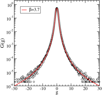
Figure 7: (color online) PDF, $G(g)$, for FRWARCH variations $\Delta S_{n}$ as a function of the scaled variable $g=(\Delta S_{n}-\big{<}\Delta S_{n}\big{>})/\sigma_{{}_{\rm A}}$, in the case $a=0.5$, $b=0.7$ and $\alpha=-0.4$. The surrogate series considered consist of $N=10^{5}$ time steps each and averages over 100 configurations were performed. The continuous line is a fit with the form: $f=f_{0}/(1+|g/g_{0}|^{\beta})$, with $f_{0}=0.51$, $g_{0}=0.86$ and $\beta=3.7$. Here, we find $\sigma_{{}_{\rm A}}\simeq 1.30$, in agreement with Eq. (24).

The fluctuation analysis of FRWARCH time series is reported in Fig. 8, where we plot the function $F(\ell)$ as a function of time scale $\ell$ for $\Delta S_{n}$ and its absolute value $|\Delta S_{n}|$, together with the behavior of the fractional process $\Delta X_{n}^{(\alpha)}$, Eq. (23). As expected, log-returns $\Delta S_{n}$ display uncorrelated behavior ($H_{\rm\Delta S}\simeq 0.5$), while the corresponding absolute returns show persistence on long time scales with an effective exponent $H_{\rm|\Delta S|}\simeq 0.8$.

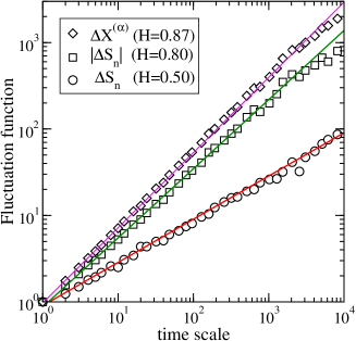
Figure 8: (color online) Fluctuation analysis for FRWARCH time series in the case $\alpha=-0.4$ (see Fig. 7). Plotted is the fluctuation function $F(\ell)/F(1)$ vs time scale $\ell$ for: Log-returns (circles), absolute log-returns (squares) and fractional random process, Eq. (23), (diamonds). The straight lines have slopes $H$ as indicated in the inset. The fluctuation analysis (FAHW) was done on a single time series of length $N=10^{5}$.

We also include the results for $\Delta X_{n}^{(\alpha)}$ indicating that for the fractional process the effective Hurst exponent, $H_{\rm\Delta X}\simeq 0.87$, is close to the expected value $H=1/2-\alpha=0.9$. We conclude that the long-time memory induced in absolute returns is a bit weaker than the one for the fractional process $\Delta X_{n}^{(\alpha)}$. However, the value of $H_{\rm|\Delta S|}\simeq 0.8$ is still consistent with the time decay of the autocorrelation function observed in empirical data for which the corresponding Hurst exponent typically varies within the range $0.7\lesssim H_{\rm|\Delta S|}\lesssim 0.9$ Roman2006 ; FBMRomanPortoPrepr .

V FIGARCH revisited

We briefly review the main properties of FIGARCH models Baillie1996 relevant for our present discussion. Let us start with the GARCH model Bollerslev:1986 , which is considered here in its simplest form. It is defined analogously to Eqs. (21) and (22), where now

$$\sigma_{n}^{2}=a+b~{}(\Delta S_{n-1})^{2}+c~{}\sigma_{n-1}^{2},$$ (25)

and $a,b,c$ are positive constants. The mean variance becomes

$$\sigma^{2}_{\mathrm{G}}=\frac{a}{1-(b+c)},$$ (26)

which is finite provided that $b+c<1$. In order to discuss the FIGARCH model, one resorts to the fractional differencing operator, defined as

$$(1-L)^{\theta} = 1-\theta L-\frac{1}{2!}\theta(1-\theta)L^{2}$$ (27)

$$~{}~{}~{}~{}~{}~{}~{}~{}~{}-\frac{1}{3!}\theta(1-\theta)(2-\theta)L^{3},\dots$$

$$= 1-\sum_{i=1}^{\infty}{\rm C}_{i}(\theta)L^{i},$$

where $0<\theta<1$, ${\rm C}_{i}(\theta)>0$ and $L$ is the lag operator, defined according to $L^{i}x^{2}_{n}=x^{2}_{n-i}$. Analogously to Eqs. (3), (8) and (9), the coefficients ${\rm C}_{i}(\theta)$ above behave for large $i$ according to

$${\rm C}_{i}(\theta)\sim{\theta\over\Gamma(1-\theta)}i^{-(1+\theta)},\qquad i\gg 1.$$ (28)

Note that ${\rm C}_{i}(\theta)=-C_{i}^{(\alpha)}$, for $\alpha>0$, as can be seen from Eq. (8). Finally, taking $L=1$ in Eq. (27), one finds the general sum-rule, $R(\theta)=\sum_{i=1}^{\infty}{\rm C}_{i}(\theta)=1$, valid for $0<\theta<1$.

The standard way of introducing FIGARCH is to write Eq. (25) using the lag operator $L$ in the form

$$(1-bL-cL)(\Delta S_{n})^{2}=a+(1-cL)[(\Delta S_{n})^{2}-\sigma_{n}^{2}],$$ (29)

and inserting the differencing operator $(1-L)^{\theta}$ in the left-hand side of the above relation, yielding,

$$(1-bL-cL)(1-L)^{\theta}(\Delta S_{n})^{2}=a+(1-cL)[(\Delta S_{n})^{2}-\sigma_{n}^{2}].$$

This is a generalization of the $\theta=1$ integrated GARCH (or IGARCH) model Baillie1996 to the case of a fractional exponent $0<\theta<1$.

Expanding the operator $(1-L)^{\theta}$ according to Eq. (27), we find

$$\sigma_{n}^{2} = a+b~{}(\Delta S_{n-1})^{2}+c~{}\sigma_{n-1}^{2}$$

$$+ \sum_{i=1}^{\infty}{\rm C}_{i}(\theta)\left[(\Delta S_{n-i})^{2}-(b+c)(\Delta S_{n-1-i})^{2}\right],$$

which, using the relation ${\rm C}_{i-1}(\theta)/{\rm C}_{i}(\theta)=i/(i-1-\theta)$, becomes

$$\sigma_{n}^{2} = a+(b+\theta)~{}(\Delta S_{n-1})^{2}+c~{}\sigma_{n-1}^{2}$$ (31)

$$+ \sum_{i=2}^{\infty}{\rm C}_{i}(\theta)~{}f_{i}(\theta,b,c)~{}(\Delta S_{n-i})^{2},$$

where

$$f_{i}(\theta,b,c)={(i-1)(1-b-c)-(\theta+b+c)\over i-1-\theta}.$$ (32)

Stability of the process is achieved when the coefficients $f_{i}(\theta,b,c)$, Eq. (32), are positive yielding the minimal condition

$$\theta+2(b+c)<1.$$ (33)

From Eq. (V), we can write the mean variance for FIGARCH as

$$\sigma^{2}_{\mathrm{F}}=\frac{a}{[1-(b+c)]~{}[1-R(\theta)]},$$ (34)

which diverges for all $0<\theta\leq 1$, because $R(\theta)=1$. In the case $0<\theta<1/2$, the autocorrelation function of $\sigma_{n}^{2}$ for a FIGARCH process decays as the power-law Baillie1996

$$\mathcal{C}(\tau)\sim|\tau|^{-(1-2\theta)},\qquad|\tau|\gg 1.$$ (35)

Writing the latter as $\mathcal{C}(\tau)\sim|\tau|^{-2(1-H)}$ (see above Eq. (17)), we find the relation $\theta=H-1/2$.

In practical calculations, the sum in Eq. (31) has a finite number of terms, with an upper memory cut-off that we denote as $M_{0}$. For finite $M_{0}$, the sum $R(\theta)<1$ and as a result the mean variance of the process is finite. In order to improve the convergence of the finite $M_{0}$ case to FIGARCH, one can use renormalized coefficients Baillie1996 ; Zumbach2004 ,

$$\tilde{\rm C}_{i}(\theta)={{\rm C}_{i}(\theta)\over\sum_{i=1}^{M_{0}}{\rm C}_{i}(\theta)},$$ (36)

so that $\tilde{R}(\theta)=\sum_{i=1}^{M_{0}}\tilde{\rm C}_{i}(\theta)=1$. The final expression for $\sigma_{n}^{2}$ then reads,

$$\sigma_{n}^{2} = a+(b+\tilde{\theta})~{}(\Delta S_{n-1})^{2}+c~{}\sigma_{n-1}^{2}$$

$$+ \sum_{i=2}^{M_{0}}\tilde{\rm C}_{i}(\theta)~{}f_{i}(\theta,b,c)~{}(\Delta S_{n-i})^{2},$$

where $\tilde{\theta}=\theta/\sum_{i=1}^{M_{0}}{\rm C}_{i}(\theta)$.

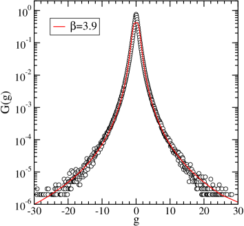
Figure 9: (color online) PDF, $G(g)$, for FIGARCH variations $\Delta S_{n}$ as a function of the scaled variable $g=(\Delta S_{n}-\big{<}\Delta S_{n}\big{>})/\sigma_{{}_{\rm F}}$, in the case $a=0.01$, $b=0.33$ and $\theta=0.3$. The surrogate series considered consist of $N=10^{5}$ time steps each, with a memory cut-off of $M_{0}=10^{5}$ time steps. (Note that each time series is actually $2N$ long, so that each of the $N$ time steps considered in the average process is a function of its previous $N$ steps.) Averages over 100 configurations were performed. The continuous line has the form: $f=f_{0}/(1+|g/g_{0}|^{\beta})$, with $f_{0}=0.42$, $g_{0}=1.08$ and $\beta=3.9$. Here, we find $\sigma_{{}_{\rm F}}\simeq 1.20$ and $\tilde{\theta}=0.307$.

In order to make contact with the FRW results discussed in Sect. IV, we consider the simpler case $c=0$ in Eq. (31), and take $a=0.01$ (in order to obtain a mean standard deviation similar to FRWARCH), $b=0.33$ (in order to get a power-law PDF as in Fig. 7) and $\theta=0.3$. The latter is chosen to yield the same value of $H=0.8$ characterizing the autocorrelation of absolute returns obtained from FRWARCH in the case $\alpha=-0.4$. Note also that the chosen value of $b$ obeys the boundary condition Eq. (33).

Results for the PDF of $\Delta S_{n}$, obtained in the case $N=M_{0}=10^{5}$, are shown in scaled form in Fig. 9. Also here, $G(g)\sim|g|^{-\beta}$, for $|g|\gg 1$, with $\beta\simeq 3.9$, similar to FRWARCH in Fig. 7. Finally, results of the fluctuation analysis are displayed in Fig. 10, supporting the expectation that for log-returns no correlations are present, while for absolute log-returns the effective Hurst exponent is consistent with $H=1/2+\theta=0.8$.

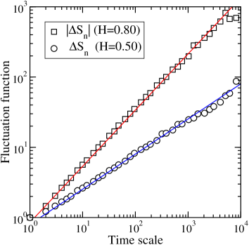
Figure 10: (color online) Fluctuation analysis for FIGARCH time series in the case $\theta=0.3$. Plotted is the fluctuation function $F(\ell)/F(1)$ vs time scale $\ell$ for: Log-returns (circles) and absolute log-returns (squares). The straight lines have slopes $H$ as indicated in the inset. The fluctuation analysis (FAHW) was done on a single time series of length $N=10^{5}$ with $M_{0}=10^{5}$ steps.

VI FIARCH revisited

There are other models currently used in literature regarding long-time memory of absolute log-returns and variable volatility. We briefly comment on them in order to better assess the impact of FRWARCH suggested here. Let us consider fractionally integrated ARCH process GrangerDing:1996 , variants of which have been studied recently Podobnik2006 ; Podobnik2007 . The model is based on the equations

$$\Delta S_{n} = \sigma_{n}\eta_{n},\qquad n\geq 1,$$ (38)

$$\sigma_{n} = \sigma_{0}\sum_{i=1}^{M_{0}}\tilde{\rm C}_{i}(\theta){|\Delta S_{n-i}|\over\big{<}|\Delta S_{n}|\big{>}},$$ (39)

where $\eta_{n}$ are independent normally distributed random numbers ($\big{<}\eta_{n}^{2}\big{>}=1$) and $0<\theta<1/2$ as for FIGARCH. According to the sum rule $\sum_{i=1}^{M_{0}}\tilde{\rm C}_{i}(\theta)=1$, see Eq. (36), Eq. (39) yields $\big{<}\sigma_{n}\big{>}=\sigma_{0}$. Thus, log-returns $\Delta S_{n}$ are uncorrelated to each other while absolute returns, $|\Delta S_{n}|$, display long-time memory. As one can see from Eq. (39), the only free parameters are $\theta$ and $\sigma_{0}$ Mzero , in contrast to the three parameters for FRWARCH. This has consequences on the shape of the PDF as we can see from the numerical results reported in Fig. 11.

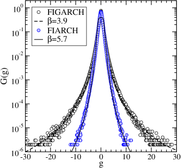
Figure 11: (color online) PDF, $G(g)$, for FIARCH variations $\Delta S_{n}$ as a function of the scaled variable $g=(\Delta S_{n}-\big{<}\Delta S_{n}\big{>})/\sigma_{{}_{\rm F}}$, in the case $\sigma_{0}=1.2$ and $\theta=0.3$ (full circles). The FIARCH series consisted of $N=10^{5}$ time steps each, with a memory cut-off of $M_{0}=10^{5}$ time steps. Averages over 100 configurations were performed. The continuous line has the form: $f=f_{0}/(1+|g/g_{0}|^{\beta})$, with $f_{0}=0.39$, $g_{0}=1.22$ and $\beta=5.7$. Here, we find $\big{<}\sigma_{n}^{2}\big{>}^{1/2}\simeq 1.30$ and $\tilde{\theta}=0.307$. For comparison, results from FIGARCH (open circles, taken from Fig. 9) have been included.

The resulting PDF for FIARCH is indeed consistent with a power-law distribution at the tails, but the power-law exponent turns out to be large, here $\beta\approx 6$, and can not be controlled by tuning a model parameter. Indeed, the value of $\theta=0.3$ is fixed by the condition that $H=0.8$. Results of fluctuation analysis for FIARCH (not shown here) confirm that in this case $H\approx 0.8$. Thus, it appears that additional degrees of freedom, in terms of model parameters, are required in Eq. (39) in order to obtain PDF with varying shapes.

To do this, we suggest a slight generalization of Eq. (39) to the form,

$$\sigma_{n}=\sigma_{0}\sum_{i=1}^{M_{0}}\tilde{\rm C}_{i}(\theta){|\Delta S_{n-i}|\over\big{<}|\Delta S_{n}|\big{>}}+b~{}|\Delta S_{n-1}|,$$ (40)

where the mean standard deviation now can be obtained as, $\big{<}\sigma_{n}\big{>}=\sigma_{0}+b~{}\big{<}|\Delta S_{n-1}|\big{>}=\sigma_{0}+b~{}\big{<}\sigma_{n-1}\big{>}\big{<}|\eta_{n-1}|\big{>}$, yielding

$$\big{<}\sigma_{n}\big{>}={\sigma_{0}\over 1-b~{}\big{<}|\eta_{n}|\big{>}}.$$ (41)

Note that for a normal distribution $\big{<}|\eta_{n}|\big{>}=\sqrt{2/\pi}\approx 0.8$.

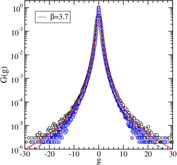
Figure 12: (color online) PDF, $G(g)$, for modified FIARCH variations $\Delta S_{n}$ as a function of the scaled variable $g=(\Delta S_{n}-\big{<}\Delta S_{n}\big{>})/\sigma_{{}_{\rm F}}$, in the case $\sigma_{0}=0.67$, $b=0.38$ and $\theta=0.3$ (full circles). The FIARCH series consisted of $N=10^{5}$ time steps each, with a memory cut-off of $M_{0}=10^{5}$ time steps. Averages over 100 configurations were performed. The dashed line has the form: $f=f_{0}/(1+|g/g_{0}|^{\beta})$, with $f_{0}=0.51$, $g_{0}=0.75$ and $\beta=3.7$. Here, we find $\big{<}\sigma_{n}^{2}\big{>}^{1/2}\simeq 1.30$ and $\tilde{\theta}=0.307$. For comparison, results from FRWARCH (open circles and continuous line, taken from Fig. 7) have been included.

Although the additional parameter $b$ actually helps in getting different decaying power-law exponents $\beta$ for the PDF, the model behaves similarly as FIGARCH in the sense that there is no an a priori way to estimate $b$ and this has to be done case by case. The numerical examples investigated (see Fig. 12) suggest that appropriate set of parameters can be found but at the expense of a numerical search.

VII Comparison to empirical data

In this section, we discuss results for FRWARCH and FIGARCH with regards to empirical data. For the latter, we take daily data for the Dow Jones Index, $I_{\rm DJ}(n)$, from 1st October 1928 till 16 May 2008 yahoo , consisting of $19994$ values. As the working variable, we consider the daily changes of the logarithm of the index, $\Delta S_{n}\equiv\ln I_{\rm DJ}(n)-\ln I_{\rm DJ}(n-1)$. The corresponding PDF is shown by the full circles in Fig. 13. To be noted is that non-stationarity issues may play a role for the Dow Jones Index as discussed in PlovdivRomanPorto . Here, we disregard such corrections and assume the series as stationary.

In the following we consider series of $N=20000$ values. Regarding FRWARCH, we use: $a=0.5$, $b=0.7$ and $\alpha=-0.4$. FIGARCH results are obtained for the case: $a=0.015$, $b=0.2$ and $\theta=0.4$ (here also $c=0$). In addition to these long-memory models, we consider for illustration a short-memory model such as the GARCH version discussed in Eq. (25), for the model parameters: $a=0.2$, $b=0.09$ and $c=0.9$. Alternatively, we will also discuss the set $b=0.9$ and $c=0.09$. Results for the PDF’s are shown in Fig. 13. To be noted is that both FRWARCH and FIGARCH yield PDF’s in good agreement with the empirical one. The results from GARCH are not that satisfactory, for the chosen set of paramters. If we take instead the alternative set ($b=0.9$ and $c=0.09$), the agreement becomes comparable to that from FRWARCH and FIGARCH. The reason for the first choice is based on the behavior of the fluctuation function for absolute returns, as we see below.

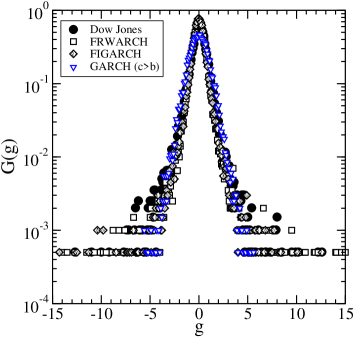
Figure 13: (color online) PDF, $G(g)$, for variations $\Delta S_{n}$ as a function of the scaled variable $g=(\Delta S_{n}-\big{<}\Delta S_{n}\big{>})/\sigma$ for: Dow Jones Index (full circles), FRWARCH (open squares), FIGARCH (filled diamonds), and GARCH (open triangles down). The model parameters are indicated in the text.

The fluctuation function of absolute log-returns for the Dow Jones Index is displayed by the full circles in Fig. 14. We find power-law behavior over about three decades with a Hurst exponent $H\simeq 0.9$, indicating a strong persistence in the autocorrelation function of absolute log-returns. Similar behavior is displayed by $|\Delta S_{n}|$ for FRWARCH (open squares), where the latter almost overlap with the empirical ones. Also FIGARCH yields results in good agreement with the Dow Jones values, although the agreement is not as good as for FRWARCH. In contrast, GARCH yields good results only for time scales below about 100 days. On larger times, the GARCH fluctuation function displays uncorrelated behavior with exponent $H=1/2$, indicating the existence of only short-range autocorrelations in the time series, as expected. If we use the second set of values (i.e. $b=0.9$ and $c=0.09$) for GARCH, the PDF improves considerably, but the fluctuation function crosses over the uncorrelated regime ($H=1/2$) already at about 10 days, yielding a poor fluctuation behavior. These results suggest that a ’long-range’ memory is a necessary ingredient in a surrogate model, as the one described by FRWARCH or FIGARCH.

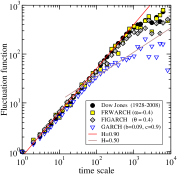
Figure 14: (color online) Fluctuation analysis versus time scale [days] of absolute returns, for: Dow Jones Index (full circles), FRWARCH (open squares), FIGARCH (filled diamonds), and GARCH (open triangles down). The straight lines have slopes $H=0.9$ and $H=0.5$, and are displayed for illustration.

VIII Conclusions

Fractional derivatives represent a conceptually simple scheme that allow us to build, from a standard random walk, stochastic processes with long-range autocorrelations. The long-memory built into the walks is controlled by the order of the fractional operator. Positive orders correspond to fractional derivatives and negative ones to fractional integrations. The former lead to fractional random walks (FRW) with negative (or anti-persistent) autocorrelations and the latter to positive (or persistent) autocorrelations. Long-time autocorrelations decay as a power-law for long time lags, the exponent of which depends on the Hurst exponent associated to the walks, the latter being a function of the fractional operator order. Examples have been studied to illustrate the use of fluctuation analysis based on Haar wavelets to determine the corresponding Hurst exponents. The results indicate that a constant Hurst exponent is consistent with a wide range of time scales, suggesting that FRW are essentially stationary for most practical purposes. A FRW model has been discussed for describing the behavior of both log-returns and their absolute values observed in empirical data of financial assets, which is based on a simple autoregressive (ARCH) scheme and denoted as FRWARCH. Absolute log-returns, as well as volatility, display strong autocorrelations, and the proposed FRW model seems to capture the essential features. Statistical properties of the present model have been compared with the predictions of a FIGARCH and FIARCH processes, to illustrate the difficulties that are found in practical calculations. We may conclude that FRWARCH turns out to be as accurate as FIGARCH regarding long-time memory features and it appears to be more stable than the latter with regard to distribution functions of log-returns. We therefore suggest that FRWARCH is suitable for simulating empirically observed slowly-decaying absolute log-returns autocorrelations, competing with the presently available models in the financial literature, as also demonstrated by a direct confrontation with daily close data from the Dow Jones Index.

References

- (1) M. Giona and H.E. Roman, Physica A 185, 87 (1992)
- (2) K.M. Kolwankar and A.D. Gangal, Phys. Rev. Lett. 80, 214 (1998)
- (3) K.B. Oldham and J. Spanier, Fractional Calculus (New York Academic, New York, 1974)
- (4) I. Podlubny, Fractional Differential Equations (Academic Press, San Diego, CA, 1999)
- (5) R. Metzler and J. Klafter, Phys. Rep. 339, 1 (2000)
- (6) R. Hilfer, Ed., Applications of Fractional Calculus in Physics (World Scientific, Singapore, 2000)
- (7) R. Gorenflo, F. Mainardi, D. Moretti and P. Paradisi, Nonlinear Dynamics 29, 129 (2002)
- (8) R. Gorenflo, F. Mainardi, D. Moretti, G. Pagnini and P. Paradisi, ArXiv preprint cond-mat/0702072v2 (2007)
- (9) R. Scherer, S.L. Kalla, L. Boyadjiev and B. Al-Saqabi, Applied Numerical Mathematics (2007) (in press).
- (10) Y.J. Campbell, A.W. Lo and A.C. Mackinlay, The Econometrics of Financial Markets (Princeton University Press, Princeton, 1997)
- (11) P. Gopikrishnan, M. Meyer, L.A.N. Amaral and H.E. Stanley, Eur. Phys. J. B 3, 139 (1998)
- (12) L. Borland, Phys. Rev. E 57, 6634 (1998)
- (13) R.N. Mantegna and H.E. Stanley, An Introduction to Econophysics (Cambridge University Press, Cambridge, 2000)
- (14) J.P. Bouchaud, A. Matacz and M. Potters, Phys. Rev. Lett. 87, 228701 (2001)
- (15) B. Podobnik, D. Fu, T. Jagric, I. Grosse and H.E. Stanley, Physica A 362, 465 (2006)
- (16) H.E. Roman, M. Albergante, M. Colombo, F. Croccolo, F. Marini and C. Riccardi, Phys. Rev. E 73, 036129 (2006)
- (17) E. Scalas, Physica A 362, 225 (2006)
- (18) J.L. McCauley, G.H. Gunaratne and K.E. Bassler, Physica A 379, 1 (2007)
- (19) R. Engle, ARCH, Selected Readings (Oxford University, Oxford, 1995)
- (20) H.E. Roman and M. Porto, Phys. Rev. E 63, 036128 (2001)
- (21) C. Dose, M. Porto and H.E. Roman, Phys. Rev. E 67, 067103 (2003)
- (22) R.F. Engle and A.J. Patton, Quantitative Finance 1, 237 (2001)
- (23) L. Palatella, J. Perelló, M. Montero and J. Masoliver, Eur. Phys. J. B 38, 671 (2004)
- (24) C.W.J. Granger, J. Econometrics 14, 227 (1980)
- (25) T. Bollerslev, J. Econometrics 31, 307 (1986)
- (26) R.F. Engle and T. Bollerslev, Econometric Review 5, 1 (1986)
- (27) R.T. Baillie, T. Bollerslev and H.O. Mikkelsen, J. Econometrics 74, 3 (1996)
- (28) G. Zumbach, Quantitative Finance 4, 70 (2004)
- (29) T.-L. Tang and S.-J. Shieh, Physica A 366, 437 (2006)
- (30) H.E. Hurst, Proc.-Inst. Civ. Eng. 1, 519 (1951)
- (31) B.B. Mandelbrot and J.W. Van Ness, SIAM Review 10, 422 (1968)
- (32) G. Samorodnitsky and M.S. Taqqu, Stable Non-Gaussian Random Processes: Stochastic Models with Infinite Variance (Chapman and Hall/CRC, Boca Raton, 1994)
- (33) D.G. Pérez, L. Zunino, M. Garavaglia and O.A. Rosso, Physica A 365, 282 (2006)
- (34) C.-K. Peng, S.V. Buldyrev, S. Havlin, M. Simons, H.E. Stanley and A.L. Goldberger, Phys. Rev. E 49, 1685 (1994)
- (35) J.W. Kantelhardt, H.E. Roman and M. Greiner, Physica A 220, 219 (1995)
- (36) E. Koscielny-Bunde, A. Bunde, S. Havlin, H.E. Roman, Y. Goldreich and H.-J. Schellnhuber, Phys. Rev. Lett. 81, 729 (1998)
- (37) Handbook of Mathematical Functions, edited by M. Abramowitz and I.A. Stegun (Dover, New York, 1972)
- (38) H.E. Roman and M. Porto, Int. J. Mod. Phys. C (2008)
- (39) The ARCH parameter is related to the decaying exponent according to RomanPorto2001 ; DosePortoRoman2003 : , yielding when .
- (40) C.W.J. Granger and Z. Ding, J. Econometrics 73, 61 (1996)
- (41) B. Podobnik, D.F. Fu, H.E. Stanley, P.Ch. Ivanov, Eur. Phys. J. B 56, 47 (2007)
- (42) The parameter is not free in the sense that it should be taken as large as possible in order that the results become independent of its value.
- (43) The historical daily data can be downloaded from: http://finance.yahoo.com/
- (44) H.E. Roman and M. Porto, Int. J. of Pure and Applied Mathematics 42, 249 (2008)