Complete Einstein metrics are geodesically rigid

Abstract

We prove that every complete Einstein (Riemannian or pseudo-Riemannian) metric $g$ is geodesically rigid: if any other complete metric $\bar{g}$ has the same (unparametrized) geodesics with $g$, then the Levi-Civita connections of $g$ and $\bar{g}$ coincide.

MSC: 83C10, 53C27, 53A20, 53B21, 53C22, 53C50, 70H06, 58J60, 53D25,70G45.

1 Introduction

1.1 Definitions and results

Let $(M^{n},g)$ be a connected Riemannian or pseudo-Riemannian manifold of dimension $n\geq 3$. We say that a metric $\bar{g}$ on $M^{n}$ is geodesically equivalent to $g$, if every geodesic of $g$ is a (reparametrized) geodesic of $\bar{g}$. We say that they are affine equivalent, if their Levi-Civita connections coincide. We say that $g$ is Einstein, if $R_{ij}=\tfrac{R}{n}\cdot g_{ij},$ where $R_{ij}$ is the Ricci tensor of the metric $g$, and $R:=R_{ij}g^{ij}$ is the scalar curvature. Our main result is

Theorem 1.

Let $g$ and $\bar{g}$ be complete geodesically equivalent metrics on a connected manifold $M^{n}$, $n\geq 3$. If $g$ is Einstein, then they are affine equivalent, or for a certain constants $c$, $\bar{c}\in\mathbb{R}$ the metrics $c\cdot g$ and $\bar{c}\cdot\bar{g}$ are Riemannian metrics of sectional curvature $1$ (and, in particular, the manifolds $(M^{n},c\cdot g)$ and $(M^{n},\bar{c}\cdot\bar{g})$ are finite quotients of the standard sphere with the standard metric).

For dimension $\geq 5$, the assumption that the metrics are complete is important: if one of them is not complete, one can construct counterexamples (essentially due to [14, 37]). For dimensions 3 and 4, (a natural modification of) Theorem 1 is true also locally:

Theorem 2.

Let $g$ and $\bar{g}$ be geodesically equivalent metrics on a connected 3- or 4-dimensional manifold $M$. If $g$ is Einstein, then they are affine equivalent, or have constant sectional curvature.

Theorem 2 was announced in [21, 39], with the extended sketch of the proof. The proof from [21, 39] is very complicated: they prolonged (= covariantly differentiated) the basic equations (8) 6 times , and used the condition that the metric is Einstein at every stage of the prolongation.

Our proof of Theorem 2 is a relatively easy Linear Algebra (inspired by [8, 13]) combined with a certain statement which is a relatively easy generalization of a certain result of Levi-Civita.

Remark 1.

Theorem 1 is also true in dimension 2 provided the scalar curvature of $g$ is constant. Without this additional assumption Theorem 1 is evidently wrong, since every 2-dimensional metric satisfies $R_{ij}=\tfrac{R}{2}\cdot g_{ij}.$

1.2 History and motivation

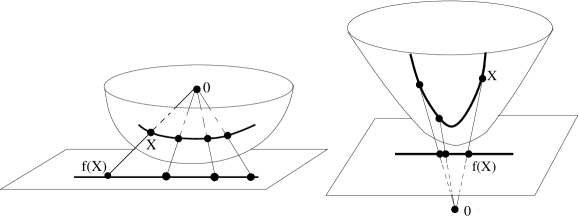
Figure 1: Surfaces of constant curvature are (locally) geodesically equivalent

The first examples of geodesically equivalent metrics are due to Lagrange [20]. He observed that the radial projection $f(x,y,z)=\left(-\frac{x}{z},-\frac{y}{z},-1\right)$ takes geodesics of the half-sphere $S^{2}:=\{(x,y,z)\in\mathbb{R}^{3}:\ \ x^{2}+y^{2}+z^{2}=1,\ z<0\}$ to the geodesics of the plane $E^{2}:=\{(x,y,z)\in\mathbb{R}^{3}:\ \ z=-1\}$, see the left-hand side of Figure 1, since geodesics of both metrics are intersection of the 2-plane containing the point $(0,0,0)$ with the surface. Later, Beltrami [5] generalized the example for the metrics of constant negative curvature, and for the pseudo-Riemannian metrics of constant curvature. In the example of Lagrange, he replaced the half sphere by the half of one of the hyperboloids $H_{\pm}^{2}:=\{(x,y,z)\in\mathbb{R}^{3}:\ \ x^{2}+y^{2}-z^{2}=\pm 1\},$ with the restriction of the Lorenz metrics $dx^{2}+dy^{2}-dz^{2}$ to it. Then, the geodesics of the metric are also intersections of the 2-planes containing the point $(0,0,0)$ with the surface, and, therefore, the stereographic projection sends it to the straight lines of the appropriate plane, see the right-hand side of Figure 1 with the (half of the) hyperboloid $H^{2}_{-}$.

Though the examples of the Lagrange and Beltrami are two-dimensional, one can easily generalize them for every dimension.

One of the possibilities in Theorem 1 is geodesically equivalent metrics of constant positive Riemannian curvature on closed manifold. Examples of such metrics are also due to Beltrami [4], we describe their natural multi-dimensional generalization. Consider the sphere

$$S^{n}\stackrel{{\scriptstyle{\rm def}}}{{=}}\{(x_{1},x_{2},...,x_{n+1})\in\mathbb{R}^{n+1}:\ x_{1}^{2}+x_{2}^{2}+...+x_{n+1}^{2}=1\}$$

with the metric $g$ which is the restriction of the Euclidean metric to the sphere. Next, consider the mapping $a:S^{n}\to S^{n}$ given by $a:v\mapsto\frac{A(v)}{\|A(v)\|}$, where $A$ is an arbitrary non-degenerate linear transformation of $\mathbb{R}^{n+1}$.

The mapping is clearly a diffeomorphism taking geodesics to geodesics. Indeed, the geodesics of $g$ are great circles (the intersections of 2-planes that go through the origin with the sphere). Since $A$ is linear, it takes planes to planes. Since the normalization $w\mapsto\frac{w}{\|w\|}$ takes punctured planes to their intersections with the sphere, the mapping $a$ takes great circles to great circles. Thus, the pullback $a^{*}g$ is geodesically equivalent to $g$. Evidently, if $A$ is not proportional to an orthogonal transformation, $a^{*}g$ is not affine equivalent to $g$.

H. Weyl was probably the first who asked (in the popular paper [51]) whether an Einstein metric can admit geodesically equivalent metric $\bar{g}$ which is nonproportional to $g$. He gave an answer (essentially due to [50]) in the pseudo-Riemannian case assuming that the metrics $g$ and $\bar{g}$ have the same light cone at every point. Later, this question was studied by many geometers and physicists (a simple search in mathscinet gives about 50 papers and few books). In particular, Petrov [41] proved that Ricci-flat 4-dimensional Einstein metrics of Lorenz signature can not be geodesically equivalent, unless they are affine equivalent. It is one of the results he obtained the Lenin prize (the most important scientific award of Soviet Union) in 1972 for. He also explicitly asked [42, Problem 5 on page 355] whether the result remains true in other dimensions.

As we will prove in Lemma 3, the assumption that the second metric is Einstein is not important, since it is automatically fulfilled. By Theorem 2, the result of Petrov remains true for 4-dimensional metrics of other signatures. As we already mentioned in Section 1.1, the counterexamples independently constructed by Mikes [37] and Formella [14] show, that the result of Petrov fails in higher dimensions (so one indeed needs certain additional assumptions, for example the assumption that the metrics are complete as in Theorem 1, which is a standard assumption in problems motivated by physics.)

Resent references include Barnes [3], Hall and Lonie [15, 18, 19], Hall [16, 17]. They studied the existence of projective transformations of Ricci-flat metrics, which is a stronger condition than the existence of geodesically equivalent metrics (projective transformations of $g$ allow to construct $\bar{g}$ geodesically equivalent to $g$. Moreover, if $g$ is Einstein, then $\bar{g}$ is automatically Einstein as well, which essentially simplifies all formulas).

One can find more historical details in the surveys [2, 12, 38] and in the introductions to the papers [28, 29, 31, 34, 35, 36].

Acknowledgments.   The results were obtained because Gary Gibbons asked the second author to check whether certain explicitly given Einstein metrics admit geodesic equivalence (these metrics admit integrals quadratic in velocities, and geodesic equivalence could lay behind the existence of such integrals, see [24, 25, 26, 27, 30, 32, 33, 43]).

There exists a algorithmic method to understand whether an explicitly given metric admits an nontrivial geodesic equivalence (assuming we can explicitly differentiate components of the metrics, and perform algebraic operations). Unfortunately, the method is highly computational, and applying it to the metrics suggested by Gibbons, which are given by quite complicated formulas, resulted so huge output, that we could not convince even ourself that everything is correct. Therefore, we started to look for a theory that could simplify the calculations, and solve the problem in the whole generality.

We thank Gary Gibbons for his question. The second author thanks Oxford, Cambridge, and Loughborough Universities, and MSRI for hospitality, and R. Bryant, A. Bolsinov, and M. Eastwood for useful discussions. Both authors were partially supported by Deutsche Forschungsgemeinschaft (Priority Program 1154 — Global Differential Geometry), and by FSU Jena.

2 Proof of Theorem 1

2.1 Schema of the proof

In Section 2.2 we list standard facts from theory of geodesically equivalent metrics, and introduce notation we will use through the paper. Most of these facts can be found in the book of Sinjukov [46], but unfortunately they are spread over the text, and it in not clear under which assumption they are true (Sinjukov always assumes real-analicity, but actually needs smoothness). All the facts could be obtained by relatively simple tensor calculations, we will indicate how.

The main result of Section 2.3 are Corollaries 3, 4. In Section 2.4 we explain that the ODE along geodesics given by Corollary 4 (that controls the reparametrization that makes $g$-geodesics from $\bar{g}$-geodesics) can not have solutions such that they satisfy the condition that both metrics are complete provided that the Einstein metric $g$ is pseudo-Riemannian, or Riemannian of nonpositive scalar curvature.

Corollary 3 will be used in Section 2.5: we will see that combining Corollary 3 with an nontrivial result of Tanno [48] immediately gives Theorem 1 under additional assumption that the metric is Riemannian of positive scalar curvature.

2.2 Standard formulas we will use

We work in tensor notations with the background metric $g$. That means, we sum with respect to repeating indexes, use $g$ for raising and lowing indexes (unless we explicitly mention), and use the Levi-Civita connection of $g$ for covariant differentiation.

As it was known already to Levi-Civita [22], two connections $\Gamma=\Gamma_{jk}^{i}$ and $\bar{\Gamma}=\bar{\Gamma}_{jk}^{i}$ have the same unparameterized geodesics, if and only if their difference is a pure trace: there exists a $(0,1)$-tensor $\phi$ such that

$$\bar{\Gamma}_{jk}^{i}=\Gamma_{jk}^{i}+\delta_{k}^{i}\phi_{j}+\delta_{j}^{i}\phi_{k}.$$ (1)

The reparameterization of the geodesics for $\Gamma$ and $\bar{\Gamma}$ connected by (1) are done according to the following rule: for a parametrized geodesic $\gamma(\tau)$ of $\bar{\Gamma}$, the curve $\gamma(\tau(t))$ is a parametrized geodesic of $\Gamma$, if and only if the parameter transformation $\tau(t)$ satisfies the following ODE:

$$\phi_{\alpha}\dot{\gamma}^{\alpha}=\frac{1}{2}\frac{d}{dt}\left(\log\left(\left|\frac{d\tau}{dt}\right|\right)\right).$$ (2)

(We denote by $\dot{\gamma}$ the velocity vector of $\gamma$ with respect to the parameter $t$, and assume summation with respect to repeating index $\alpha$.)

If $\Gamma$ and $\bar{\Gamma}$ related by (1) are Levi-Cevita connections of metrics $g$ and $\bar{g}$, then one can find explicitly (following Levi-Civita [22]) a function $\phi$ on the manifold such that its differential $\phi_{,i}$ coincides with the covector $\phi_{i}$: indeed, contracting (1) with respect to $i$ and $j$, we obtain $\bar{\Gamma}_{\alpha i}^{\alpha}=\Gamma_{\alpha i}^{\alpha}+(n+1)\phi_{i}$. From the other side, for the Levi-Civita connection $\Gamma$ of a metric $g$ we have $\Gamma_{\alpha k}^{\alpha}=\tfrac{1}{2}\frac{\partial\log(|det(g)|)}{\partial x_{k}}$. Thus,

$$\phi_{i}=\frac{1}{2(n+1)}\frac{\partial}{\partial x_{i}}\log\left(\left|\frac{\det(\bar{g})}{\det(g)}\right|\right)=\phi_{,i}$$ (3)

for the function $\phi:M\to\mathbb{R}$ given by

$$\phi:=\frac{1}{2(n+1)}\log\left(\left|\frac{\det(\bar{g})}{\det(g)}\right|\right).$$ (4)

In particular, the derivative of $\phi_{i}$ is symmetric, i.e., $\phi_{i,j}=\phi_{j,i}$.

The formula (1) implies that two metrics $g$ and $\bar{g}$ are geodesically equivalent if and only if for a certain $\phi_{i}$ (which is, as we explained above, the differential of $\phi$ given by (4)) we have

$$\bar{g}_{ij,k}-2\bar{g}_{ij}\phi_{k}-\bar{g}_{ik}\phi_{j}-\bar{g}_{jk}\phi_{i}=0,$$ (5)

where “comma” denotes the covariant derivative with respect to the connection $\Gamma$. Indeed, the left-hand side of this equation is the covariant derivative with respect to $\bar{\Gamma}$, and vanishes if and only if $\bar{\Gamma}$ is the Levi-Civita connection for $\bar{g}$.

The equations (5) can be linearized by a clever substitution: consider $a_{ij}$ and $\lambda_{i}$ given by

$$a_{ij} = e^{2\phi}\bar{g}^{\alpha\beta}g_{\alpha i}g_{\beta j},$$ (6)

$$\lambda_{i} = -e^{2\phi}\phi_{\alpha}\bar{g}^{\alpha\beta}g_{\beta i},$$ (7)

where $\bar{g}^{\alpha\beta}$ is the tensor dual to $\bar{g}_{\alpha\beta}$:  $\bar{g}^{\alpha i}\bar{g}_{\alpha j}=\delta_{j}^{i}$. It is an easy exercise to show that the following linear equations on the symmetric $(0,2)-$tensor $a_{ij}$ and $(0,1)-$tensor $\lambda_{i}$ are equivalent to (5).

$$a_{ij,k}=\lambda_{i}g_{jk}+\lambda_{j}g_{ik}.$$ (8)

Remark 2.

For dimension 2, the substitution (6,7) was already known to R. Liouville [23] and Dini [11], see [9, Section 2.4] for details and a conceptual explanation. For arbitrary dimension, the substitution (6,7) and the equation (8) are due to Sinjukov [46]. Geometry staying behind is explained in [13].

Note that it is possible to find a function $\lambda$ such that its differential is precisely the the $(0,1)-$tensor $\lambda_{i}$: indeed, multiplying (8) by $g^{ij}$ and summing with respect to repeating indexes $i,j$ we obtain $(g^{ij}a_{ij})_{,k}=2\lambda_{k}$. Thus, $\lambda_{i}$ is the differential of the function

$$\lambda:=\tfrac{1}{2}g^{\alpha\beta}a_{\alpha\beta}.$$ (9)

In particular, the covariant derivative of $\lambda_{i}$ is symmetric: $\lambda_{i,j}=\lambda_{j,i}$.

Integrability conditions for the equation (8) (we substitute the derivatives of $a_{ij}$ given by (8) in the formula $a_{ij,lk}-a_{ij,kl}=a_{i\alpha}R^{\alpha}_{jkl}+a_{\alpha j}R^{\alpha}_{ikl}$, which is true for every $(0,2)-$tensor $a_{ij}$) were first obtained by Solodovnikov [47] and are

$$a_{i\alpha}R^{\alpha}_{jkl}+a_{\alpha j}R^{\alpha}_{ikl}=\lambda_{l,i}g_{jk}+\lambda_{l,j}g_{ik}-\lambda_{k,i}g_{jl}-\lambda_{k,j}g_{il}.$$ (10)

For further use let us recall the fact which can also be obtained by simple calculations: the Ricci-tensors of connections related by (1) are connected by the formula

$$\bar{R}_{ij}=R_{ij}-(n-1)(\phi_{i,j}-\phi_{i}\phi_{j}),$$ (11)

where $R_{ij}$ is the Ricci-tensor of $\Gamma$ and $\bar{R}_{ij}$ is the Ricci-tensor of $\bar{\Gamma}$.

2.3 Local results

Within the whole paper we work on a smooth manifold of dimension $n\geq 3$.

Lemma 1 (Folklore).

Let $a_{ij}$ be a solution of (8) for the metric $g$. Then, it commutes with the Ricci-tensor:

$$a^{\alpha}_{i}R_{\alpha j}=a^{\alpha}_{j}R_{i\alpha}.$$ (12)

Proof. Consider the equations (10). We “cycling” the equation with respect to $i,k,l$: we sum it with itself after renaming the indexes according to $(i\mapsto k\mapsto l\mapsto i)$ and with itself after renaming the indexes according to $(i\mapsto l\mapsto k\mapsto i)$. The first term at the left-hand side of the equation will disappear because of the Bianchi equality $R^{\alpha}_{ikl}+R^{\alpha}_{kli}+R^{\alpha}_{lik}=0$, the right-hand side vanishes completely, and we obtain

$$a_{\alpha i}R^{\alpha}_{jkl}+a_{\alpha k}R^{\alpha}_{jli}+a_{\alpha l}R^{\alpha}_{jik}=0.$$ (13)

Multiplying with $g^{jk}$, using the symmetries of the curvature tensor, and summing over the repeating indexes we obtain $a_{\alpha i}R^{\alpha}_{l}-a_{\alpha l}R^{\alpha}_{i}=0$ implying the claim, ∎

Lemma 2.

Suppose the curvature tensor of the metric $g$ satisfies

$$R^{\alpha}_{ijk,\alpha}=0.$$

Then, for every solution $a_{ij}$ of (8) such that $\lambda_{i}\neq 0$ at a point $p\in M^{n}$, in a sufficiently small neighborhood $U(p)$ of $p$ we have

$$\lambda_{k,j}=\stackrel{{\scriptstyle 1}}{{c}}g_{kj}+\stackrel{{\scriptstyle 2}}{{c}}R_{kj}+\stackrel{{\scriptstyle 3}}{{c}}a_{kj}+\stackrel{{\scriptstyle 4}}{{c}}a^{\alpha}_{j}R_{\alpha k},$$ (14)

where the coefficients $\stackrel{{\scriptstyle 1}}{{c}}$, $\stackrel{{\scriptstyle 2}}{{c}}$, $\stackrel{{\scriptstyle 3}}{{c}}$, $\stackrel{{\scriptstyle 4}}{{c}}$ are given by the formulas

$$\stackrel{{\scriptstyle 1}}{{c}}=\frac{-\lambda_{\alpha}a^{\alpha}_{\beta}\xi^{\beta}R+2\lambda\lambda^{\ \ \ \beta}_{\alpha,\beta}\xi^{\alpha}+a^{\alpha}_{\beta}R^{\beta}_{\alpha}-4\lambda_{\alpha,}^{\ \ \alpha}}{4n};\ \ \stackrel{{\scriptstyle 2}}{{c}}=\tfrac{1}{4}\lambda_{\alpha}a^{\alpha}_{\beta}\xi^{\beta};\ \ \stackrel{{\scriptstyle 3}}{{c}}=-\tfrac{1}{4}\lambda^{\ \ \ \beta}_{\alpha,\beta}\xi^{\alpha};\stackrel{{\scriptstyle 4}}{{c}}=-\tfrac{1}{4}a^{\alpha}_{\beta}R_{\alpha}^{\beta},$$

where $\xi$ is an arbitrary vector field such that $\lambda_{i}\xi^{i}=1$.

Remark 3.

The assumptions of the lemma are automatically fulfilled for Einstein spaces. Indeed, the second Bianchi identity for the curvature tensor is

$$R^{h}_{ijk,l}+R^{h}_{ikl,j}+R^{h}_{ilj,k}=0.$$

Contracting with respect to $h$ and $l$, we obtain

$$R^{\alpha}_{ijk,\alpha}+\underbrace{R^{\alpha}_{ik\alpha,j}}_{-R_{ik,j}}+\underbrace{R^{\alpha}_{i\alpha j,k}}_{R_{ij,k}}=0.$$

If the metric is Einstein, then the second and the third components of the equation vanishes, and we obtain $R^{\alpha}_{ijk,\alpha}=0$. Moreover, we see that actually the condition $R_{ik,j}-R_{ij,k}=0$ is a necessary and sufficient condition for $R^{\alpha}_{ijk,\alpha}=0$.

Remark 4.

The tensor $R_{ik,j}-R_{ij,k}$ is called projective Yano tensor, and plays important role in the theory of geodesically equivalent metrics; in particular, it is projectively invariant in dimension 2 [23, 9], and is an essential part of the so-called tractor approach for the investigation of geodesically equivalent metrics [13].

Proof of Lemma 2. Consider the solution $a_{ij}$ of the equation (8). Let us take the covariant derivative of the equations (10) (the index of differentiation is “$m$”), and replace the covariant derivative of $a$ by formula (8). We obtain

$$\begin{array}[]{l}\ \ \ \lambda_{\alpha}R^{\alpha}_{jkl}g_{im}+\lambda_{i}R_{mjkl}+a_{\alpha i}R^{\alpha}_{jkl,m}+\lambda_{\alpha}R^{\alpha}_{ikl}g_{jm}+\lambda_{j}R_{mikl}+a_{\alpha j}R^{\alpha}_{ikl,m}\\ =\lambda_{l,im}g_{jk}+\lambda_{l,jm}g_{ik}-\lambda_{k,im}g_{jl}-\lambda_{k,jm}g_{il}.\end{array}$$ (15)

We multiply with $g^{lm}$, sum with respect to repeating indexes $l,m$, and use $R^{\alpha}_{ijk,\alpha}=0.$ We obtain:

$$\lambda_{\alpha}R^{\alpha}_{ikj}+\lambda_{\alpha}R^{\alpha}_{jki}-\lambda_{i}R_{jk}-\lambda_{j}R_{ik}=\lambda^{\ \ \ \alpha}_{i,\alpha}g_{jk}+\lambda^{\ \ \ \alpha}_{j,\alpha}g_{ik}-\lambda_{k,ij}-\lambda_{k,ji}.$$ (16)

We now alternate the equation (16) with respect to $k,j$ to obtain

$$\begin{array}[]{l}\ \ \ 4\lambda_{\alpha}R^{\alpha}_{ikj}=\lambda^{\ \ \ \alpha}_{j,\alpha}g_{ik}-\lambda^{\ \ \ \alpha}_{k,\alpha}g_{ij}-\lambda_{k}R_{ij}+\lambda_{j}R_{ik}.\end{array}$$ (17)

Let us now rename the indexes $i\mapsto k\mapsto j\mapsto\alpha$ in (17), multiply the result by $a^{\alpha}_{i}$, use the symmetries of the curvature tensor and sum over the repeating index $\alpha$. We obtain

$$\begin{array}[]{lcl}\ \ \ 4a^{\alpha}_{i}R_{\alpha jk\beta}\lambda^{\beta}&=&4a^{\alpha}_{i}R_{kj\alpha}^{\beta}\lambda_{\beta}\\ &=&a^{\alpha}_{i}\left(\lambda^{\ \ \ \beta}_{\alpha,\beta}g_{kj}-\lambda^{\ \ \ \alpha}_{k,\alpha}g_{ij}-\lambda^{\ \ \ \beta}_{j,\beta}g_{k\alpha}-\lambda_{j}R_{\alpha k}+\lambda_{\alpha}R_{jk}\right)\\ &=&a^{\alpha}_{i}\lambda^{\ \ \ \beta}_{\alpha,\beta}g_{kj}-\lambda^{\ \ \ \beta}_{j,\beta}a_{ki}-\lambda_{j}a^{\alpha}_{i}R_{\alpha k}+\lambda_{\alpha}a^{\alpha}_{i}R_{kj}.\end{array}$$ (18)

Now we multiply the equation (10) by $\lambda^{l}$ and sum over the repeating index $l$. We see that the first component of the result is precisely the left-hand side of (18); we replace it by the right-hand side of (18). We obtain

$$\begin{array}[]{lll}0&=&\left(a^{\alpha}_{i}\lambda^{\ \ \ \beta}_{\alpha,\beta}-4\lambda^{\alpha}\lambda_{\alpha,i}\right)g_{kj}-\lambda^{\ \ \ \beta}_{j,\beta}a_{ki}+\lambda_{j}\left(-a^{\alpha}_{i}R_{\alpha k}+4\lambda_{k,i}\right)+\lambda_{\alpha}a^{\alpha}_{i}R_{kj}\\ &+&\left(a^{\alpha}_{j}\lambda^{\ \ \ \beta}_{\alpha,\beta}-4\lambda^{\alpha}\lambda_{\alpha,j}\right)g_{ki}-\lambda^{\ \ \ \beta}_{i,\beta}a_{kj}+\lambda_{i}\left(-a^{\alpha}_{j}R_{\alpha k}+4\lambda_{k,j}\right)+\lambda_{\alpha}a^{\alpha}_{j}R_{ki}\end{array}$$ (19)

We now alternate (18) with respect to $k,j$, rename $k\longleftrightarrow i$, and add the result to (19). After dividing by 2 for cosmetic reasons, and using that by Lemma 1 the tensor $a^{\alpha}_{i}R_{\alpha k}$ is symmetric with respect to $i,k$, we obtain

$$\left(a^{\alpha}_{i}\lambda^{\ \ \ \beta}_{\alpha,\beta}-4\lambda^{\alpha}\lambda_{\alpha,i}\right)g_{kj}+\lambda_{\alpha}a^{\alpha}_{i}R_{kj}-\lambda^{\ \ \ \beta}_{i,\beta}a_{kj}+\lambda_{i}\left(-a^{\alpha}_{j}R_{\alpha k}+4\lambda_{k,j}\right)=0.$$ (20)

We multiply (20) by $g^{kj}$ and sum over the repeating indexes $k,j$. We obtain (after dividing by $n$)

$$\left(a^{\alpha}_{i}\lambda^{\ \ \ \beta}_{\alpha,\beta}-4\lambda^{\alpha}\lambda_{\alpha,i}\right)=-\tfrac{R}{n}\lambda_{\alpha}a^{\alpha}_{i}+\frac{2\lambda}{n}\lambda^{\ \ \ \beta}_{i,\beta}-\lambda_{i}\frac{\left(-a^{\alpha}_{\beta}R_{\alpha}^{\beta}+4\lambda_{\alpha,}^{\ \ \alpha}\right)}{n}=0,$$ (21)

where $R:=R_{\alpha\beta}g^{\alpha\beta}$ is the scalar curvature of $g$. Substituting the expression for $\left(a^{\alpha}_{i}\lambda^{\ \ \ \beta}_{\alpha,\beta}-4\lambda^{\alpha}\lambda_{\alpha,i}\right)$ from (21) in (20), we obtain

$$\begin{array}[]{ccl}0&=&\lambda_{\alpha}a^{\alpha}_{i}\left(R_{kj}-\tfrac{R}{n}g_{kj}\right)+\lambda_{i,\beta}^{\ \ \ \beta}\left(\frac{2\lambda}{n}g_{kj}-a_{kj}\right)\\ &-&\lambda_{i}\left(\frac{-a^{\alpha}_{\beta}R_{\alpha}^{\beta}+4\lambda_{\alpha,}^{\ \ \alpha}}{n}g_{kj}+a^{\alpha}_{j}R_{\alpha k}-4\lambda_{k,j}\right)\end{array}$$ (22)

Since $\lambda_{i}\neq 0$ at a point $p$, then $\lambda_{i}\xi^{i}=1$ for a certain vector field $\xi$ in a sufficiently small neighborhood $U(p)$. Contracting the equation (22) with this $\xi^{i}$, we obtain

$$\begin{array}[]{ccl}0&=&\lambda_{\alpha}a^{\alpha}_{i}\xi^{i}\left(R_{kj}-\tfrac{R}{n}g_{kj}\right)+\xi^{i}\lambda_{i,\beta}^{\ \ \beta}\left(\frac{2\lambda}{n}g_{kj}-a_{kj}\right)\\ &-&\lambda_{i}\left(\frac{-a^{\alpha}_{\beta}R_{\alpha}^{\beta}+4\lambda_{\alpha,}^{\ \ \ \alpha}}{n}g_{kj}+a^{\alpha}_{j}R_{\alpha k}-4\lambda_{k,j}\right)\end{array}$$ (23)

We see that $\lambda_{j,k}$ is a linear combination of $a^{\alpha}_{j}R_{\alpha k}$, $g_{jk}$, $R_{jk}$ and $a_{kj}$ as we want. The coefficients in the linear combination are as in the formula below , ∎

$$4\lambda_{k,j}=a_{\alpha k}R^{\alpha}_{j}+\frac{-\lambda_{\alpha}a^{\alpha}_{\beta}\xi^{\beta}R+2\lambda\lambda^{\ \ \ \beta}_{\alpha,\beta}\xi^{\alpha}+a^{\alpha}_{\beta}R^{\beta}_{\alpha}-4\lambda_{\alpha}^{\alpha}}{n}g_{jk}+\lambda_{\alpha}a^{\alpha}_{\beta}\xi^{\beta}R_{jk}-\lambda^{\ \ \ \beta}_{\alpha,\beta}\xi^{\alpha}a_{kj}.$$

Corollary 1.

Assume $g$ is an Einstein metric. Let $a_{ij}$ be a solution of (8). Assume $\lambda_{i}\neq 0$ at a point $p$. Then, in a sufficiently small neighborhood of $p$, $\lambda_{i,j}$ is a linear combination of $g_{ij}$ and $a_{ij}$:

$$\lambda_{i,j}=\mu g_{ij}+Ka_{ij},$$ (24)

where the coefficients $K:=-\tfrac{R}{n(n-1)}$ and $\mu:=\frac{\lambda_{\alpha,}^{\ \alpha}-2K\lambda}{n}$.

Proof. By assumption, in a small neighborhood of $p$ we have $\lambda_{i}\neq 0$; this implies that $a_{ij}$ is not proportional to $g_{ij}$, because by the result of Weyl [50] if two metrics are geodesically and conformally equivalent, then they are proportional (with a constant coefficient of proportionality).

As we explained in Remark 3, the assumptions of the lemma are fullfilled if the metric is Einstein. Moreover, if the metric is Einstein, then the second term of the right-hand side of (14) is proportional to $g$, and the last term is proportional to $a$ implying that $\lambda_{i,j}$ is a linear combination of $g_{ij}$ and $a_{ij}$. We need to calculate the coefficients of the linear combination.

Substituting the condition that the metric is Einstein in (17) we obtain

$$\begin{array}[]{l}\lambda_{\alpha}R^{\alpha}_{ikj}=\tau_{j}g_{ik}-\tau_{k}g_{ij},\end{array}$$ (25)

where

$$\tau_{i}:=\tfrac{1}{4}\left(\lambda_{i,\alpha}^{\ \ \ \alpha}+\tfrac{R}{n}\lambda_{i}\right).$$ (26)

Contracting the equation (26) with $g^{ij}$ we obtain $(n-1)\tau_{j}=-\tfrac{R}{n}\lambda_{j}$ implying

$$\tau_{j}=-\tfrac{R}{n(n-1)}\lambda_{j}.$$ (27)

Now, since the metric is Einstein, the first bracket in the sum (22) is zero, and the term $a^{\alpha}_{\beta}R_{\alpha}^{\beta}$ equals $\tfrac{R}{n}\delta_{\alpha}^{\beta}a^{\alpha}_{\beta}=2\tfrac{R}{n}\lambda$, so the formula (22) reads

$$\lambda_{i,\beta}^{\ \ \ \beta}\left(\frac{2\lambda}{n}g_{kj}-a_{kj}\right)-\lambda_{i}\left(\frac{-2\lambda\tfrac{R}{n}+4\lambda_{\alpha,}^{\ \alpha}}{n}g_{kj}+\tfrac{R}{n}a_{kj}-4\lambda_{k,j}\right)=0$$ (28)

Combining (26) and (27), we obtain

$$\lambda_{i,\beta}^{\ \ \ \beta}=\left(4k-\tfrac{R}{n}\right)\lambda_{i}.$$ (29)

Substituting this in (28), we obtain

$$\left(4k-\tfrac{R}{n}\right)\left(\frac{2\lambda}{n}g_{kj}-a_{kj}\right)\lambda_{i}-\left(\frac{-2\lambda\tfrac{R}{n}+4\lambda_{\alpha,}^{\ \alpha}}{n}g_{kj}+\tfrac{R}{n}a_{kj}-4\lambda_{k,j}\right)\lambda_{i}=0.$$ (30)

Since by assumption $\lambda_{i}\neq 0$, we obtain (24), ∎

Remark 5.

Assume $g$ is an Einstein metric. Let $a_{ij}$ be a solution of (8). Then,

$$\lambda_{\alpha}Y^{\alpha}_{ijk}=0,$$ (31)

where $Y^{h}_{ijk}:=R^{h}_{ijk}-\tfrac{R}{n(n-1)}\left(\delta^{h}_{j}g_{ik}-\delta^{h}_{k}g_{ij}\right)$ is the so-called concircular curvature of $g$ introduced by Yano [52].

Proof. Substituting (27) in (25), we obtain the claim, ∎

Corollary 2.

Assume $g$ is an Einstein metric. Let $a_{ij}$ be a solution of (8). Consider $K:=-\tfrac{R}{n(n-1)}$ and the function $\mu:=\frac{\lambda_{\alpha,}^{\ \ \alpha}-2K\lambda}{n}$. Then, the function $\mu$ satisfies the equation

$$\mu_{,i}=2K\lambda_{i}.$$ (32)

Remark 6.

In particular, under the assumptions of Corollary 2, for a certain $\mbox{\rm const}\in\mathbb{R}$, the function $\lambda+\mbox{\rm const}$ is an eigenfunction of the laplacian of $g$.

Proof of Corollary 2. If $\lambda$ is constant in a neighborhood of a point, the equation (32) is automatically fulfilled. Below we will assume that $\lambda$ is not constant. Differentiating the definition of $\mu$ and multiplying by $n$ for cosmetic reasons, we obtain

$$n\mu_{,i}=2\lambda_{\alpha,\ i}^{\ \ \alpha}-2K\lambda_{i}.$$ (33)

By definition of curvature we have $\lambda_{i,jk}-\lambda_{i,kj}=\lambda_{\alpha}R^{\alpha}_{ijk}$. Contracting this with $g^{ij}$, and using $R_{ij}=\tfrac{R}{n}g_{ij}$, we obtain

$$\lambda_{\alpha,\ \ k}^{\ \ \alpha}-\lambda_{k,\alpha}^{\ \ \ \alpha}=-\tfrac{R}{n}\lambda_{k}.$$

The formula (29) gives us $\lambda_{k,\alpha}^{\ \ \ \alpha}$, whose substitution gives

$$\lambda_{\alpha,\ k}^{\ \ \alpha}=\left(-2\tfrac{R}{n}+4K\right)\lambda_{k}.$$

Substituting this in (33), we obtain $\mu_{,i}=-\tfrac{2R}{n(n-1)}\lambda_{i}=2K\lambda_{i},$ ∎

Corollary 3.

Let $g$ and $\bar{g}$ be geodesically equivalent metrics, assume $g$ is an Einstein metric. Then, the function $\lambda$ given by (9) satisfies

$$\lambda_{,ijk}-K\cdot\left(2\lambda_{,k}g_{ij}+\lambda_{,j}g_{ik}+\lambda_{,i}g_{jk}\right)=0,$$ (34)

where $K:=-\tfrac{R}{n(n-1)}$.

Proof. If $\lambda$ is constant in a neighborhood of $p$, the equation is automatically fulfilled. Then, it is sufficient to prove Corollary 3 at points $p$ such that $\lambda_{i}(p)\neq 0$.

Covariantly differentiating (24), we obtain $\lambda_{i,jk}=\mu_{,k}g_{ij}+Ka_{ij,k}$. Substituting $\mu_{,k}$ by (32), and $a_{ij,k}$ by (8), we obtain the claim, ∎

Lemma 3.

Let $g$ and $\bar{g}$ be geodesically equivalent. Assume $g$ is Einstein, and assume that $\lambda_{i}\neq 0$ at a point $p$.

Then, the restriction of $\bar{g}$ to a sufficiently small neighborhood $U(p)$ is Einstein as well. Moreover, the following formula holds (at every point of $U(p)$).

$$\phi_{i,j}-\phi_{i}\phi_{j}=\tfrac{R}{n(n-1)}g_{ij}-\tfrac{\bar{R}}{n(n-1)}\bar{g}_{ij},$$ (35)

where $\bar{R}$ is the scalar curvature of the metric $\bar{g}$.

Proof. We covariantly differentiate (7) (the index of differentiation is “j”); then we substitute the expression (5) for $\bar{g}_{ij,k}$ to obtain

$$\begin{array}[]{ccl}\lambda_{i,j}&=&-2e^{2\phi}\phi_{j}\phi_{\alpha}\bar{g}^{\alpha\beta}g_{\beta i}-e^{2\phi}\phi_{\alpha,j}\bar{g}^{\alpha\beta}g_{\beta i}+e^{2\phi}\phi_{\alpha}\bar{g}^{\alpha\gamma}\bar{g}_{\gamma l,j}\bar{g}^{l\beta}g_{\beta i}\\ &=&-e^{2\phi}\phi_{\alpha,j}\bar{g}^{\alpha\beta}g_{\beta i}+e^{2\phi}\phi_{\alpha}\phi_{\gamma}\bar{g}^{\alpha\gamma}\bar{g}_{ij}+e^{2\phi}\phi_{j}\phi_{l}\bar{g}^{l\beta}g_{\beta i}\end{array},$$ (36)

where $\bar{g}^{\alpha\beta}$ is the tensor dual to $\bar{g}_{\alpha\beta}$. We now substitute $\lambda_{i,j}$ from (24), use that $a_{ij}$ is given by (6), and divide by $e^{2\phi}$ for cosmetic reasons to obtain

$$e^{-2\phi}\mu g_{ij}+K\bar{g}^{\alpha\beta}g_{\alpha j}g_{\beta_{i}}=-\phi_{\alpha,j}\bar{g}^{\alpha\beta}g_{\beta i}+\phi_{\alpha}\phi_{\gamma}\bar{g}^{\alpha\gamma}\bar{g}_{ij}+\phi_{j}\phi_{l}\bar{g}^{l\beta}g_{\beta i}.$$ (37)

Multiplying with $g^{i\xi}\bar{g}_{\xi k}$, we obtain

$$\phi_{k,j}-\phi_{k}\phi_{j}=(\phi_{\alpha}\phi_{\beta}\bar{g}^{\alpha\beta}-e^{-2\phi}\mu)\bar{g}_{kj}-Kg_{kj}.$$ (38)

Let us now show that the coefficient ${\bar{K}}{}:=-\tfrac{\phi_{\alpha}\phi_{\beta}\bar{g}^{\alpha\beta}-e^{-2\phi}\mu}{n-1}$ is constant. Substituting (38) in (11), and using $R_{ij}=\tfrac{R}{n}g_{ij}$, we obtain

$$\bar{R}_{ij}=\tfrac{R}{n}g_{ij}-\tfrac{R}{n}g_{ij}-(\phi_{\alpha}\phi_{\beta}\bar{g}^{\alpha\beta}-e^{-2\phi}\mu)\bar{g}_{ij}.$$

We see that $\bar{R}_{ij}$ is proportional to $\bar{g}_{ij}$. Then, $\bar{g}$ is an Einstein metric; in particular, $\bar{K}:=-\tfrac{\phi_{\alpha}\phi_{\beta}\bar{g}^{\alpha\beta}-e^{-2\phi}\mu}{n-1}$ is a constant equal to $-\tfrac{\bar{R}}{n(n-1)}$, and (38) gives us the formula

$$\bar{K}\bar{g}_{ij}=Kg_{ij}+\phi_{i,j}-\phi_{i}\phi_{j},$$ (39)

which is evidently equivalent to (35), ∎

Corollary 4.

Let $g$ and $\bar{g}$ be geodesically equivalent metrics, assume $g$ is an Einstein metric. Consider a (parametrized) geodesic $\gamma$ of the metric $g$, and denote by $\dot{\phi}$, $\ddot{\phi}$ and $\dddot{\phi}$ the first, second and third derivatives of the function $\phi$ given by (4) along the geodesic. Then, along the geodesic, the following ordinary differential equation holds:

$$\begin{array}[]{lcl}\dddot{\phi}&=&4Kg(\dot{\gamma},\dot{\gamma})\dot{\phi}+6\dot{\phi}\ddot{\phi}-4(\dot{\phi})^{3}\end{array},$$ (40)

where $g(\dot{\gamma},\dot{\gamma}):=g_{ij}\dot{\gamma}^{i}\dot{\gamma}^{j}$.

Proof. If $\phi\equiv 0$ in a neighborhood $U$, the equation is automatically fulfilled. Then, it is sufficient to prove Corollary 4 assuming $\phi_{i}$ is not constant.

The formula (35) is evidently equivalent to (39), which is evidently equivalent to

$$\phi_{i,j}=\bar{K}\bar{g}_{ij}-Kg_{ij}+\phi_{i}\phi_{j}.$$ (41)

Taking covariant derivative of (41), we obtain

$$\phi_{i,jk}=\bar{K}\bar{g}_{ij,k}+2\phi_{i,k}\phi_{j}+2\phi_{j,k}\phi_{i}.$$ (42)

Substituting the expression for $\bar{g}_{ij,k}$ from (5), and substituting $\bar{K}\bar{g}_{ij}$ given by (39), we obtain

$$\begin{array}[]{lcl}\phi_{i,jk}&=&\bar{K}(2\bar{g}_{ij}\phi_{k}+\bar{g}_{ik}\phi_{j}+\bar{g}_{jk}\phi_{i})+2\phi_{i,k}\phi_{j}+2\phi_{j,k}\phi_{i}\\ &=&K(2g_{ij}\phi_{k}+g_{ik}\phi_{j}+g_{jk}\phi_{i})+2(\phi_{k}\phi_{i,j}+\phi_{i}\phi_{j,k}+\phi_{j}\phi_{k,i})-4\phi_{i}\phi_{j}\phi_{k}\end{array}$$ (43)

Contracting with $\dot{\gamma}^{i}\dot{\gamma}^{j}\dot{\gamma}^{k}$ and using that $\phi_{i}$ is the differential of the function (4) we obtain the desired ODE (40), ∎

Corollary 5.

Let $\bar{g}$ (on a connected $M^{n\geq 3})$ be geodesically equivalent to an Einstein metric $g$, but is not affine equivalent ot $g$. Then, the restrictions of $g$ and $\bar{g}$ to any neighborhood are also not affine equivalent.

Remark 7.

The assumption that $g$ is Einstein is important: Levi-Civita’s description of geodesically equivalent metrics [22] immediately gives counterexamples.

Proof of Corollary 5. Suppose $\phi_{i}\neq 0$ at a point $p$. Consider a geodesic $\gamma(t)$ such that $\gamma(0)=p$, $\dot{\gamma}^{\alpha}(0)\phi_{\alpha}\neq 0$. By Lemma 4, the function $\phi_{i}\dot{\gamma}^{i}$ satisfies equation (40) along the geodesic. Since $\dot{\phi}(0)\neq 0$, then $\dot{\phi}(t)\neq 0$ for almost every $t$. Then, $\phi_{i}\neq 0$ at almost every point of geodesic. Since every point can be reached from the point $p$ by a sequence of geodesics, $\phi_{i}\neq 0$ at almost every point, ∎

2.4 Proof of Theorem 1 for Riemannian metrics of nonpositive scalar curvature, and for pseudo-Riemannian metrics

Assume the metric $g$ on a connected $M^{n\geq 3}$ is Einstein and is either Riemannian (i.e., positive defined) with nonpositive scalar curvature, or essentially pseudo-Riemannian (i.e., there exists light-like vectors). Let $\bar{g}$ be geodesically equivalent to $g$. Assume both metrics are complete. Our goal is to show that $\phi$ given by (4) is constant, because in view of (1) this implies that the metrics are affine equivalent.

Consider a parameterized geodesic $\gamma(t)$ of $g$. If the metric $g$ is pseudo-Riemannian, we additionally assume that $\gamma$ is a light-like geodesic i.e., $\dot{\gamma}^{i}\dot{\gamma}^{j}g_{ij}=0$. Since the metrics are geodesically equivalent, for a certain function $\tau:\mathbb{R}\to\mathbb{R}$ the curve $\gamma(\tau)$ is a geodesic of $\bar{g}$. Since the metrics are complete, the reparameterization $\tau(t)$ is a diffeomorphism $\tau:\mathbb{R}\to\mathbb{R}$. Without loss of generality we can think that $\dot{\tau}:=\frac{d}{dt}\tau$ is positive, otherwise we replace $t$ by $-t$. Then, the equation (2) along the geodesic reads

$$\phi(t)=\tfrac{1}{2}\log(\dot{\tau}(t))+\mbox{\rm const}_{0}.$$ (44)

Now let us consider the equation (40). Substituting

$$\phi(t)=-\tfrac{1}{2}\log(p(t))+\mbox{\rm const}_{0}$$ (45)

in it (since $\dot{\tau}>0$, the substitution is global), we obtain

$$\dddot{p}=4Kg(\dot{\gamma},\dot{\gamma})\dot{p}.$$ (46)

Since the length of the tangent vector is preserved along a geodesic, $g(\dot{\gamma},\dot{\gamma})$, and therefore $4Kg(\dot{\gamma},\dot{\gamma})$ is a constant. The assumptions above imply that this constant is nonnegative.

Indeed, if the metric is essentially pseudo-Riemannian, this constant is zero, since $\gamma$ is an light-like geodesic. If the metric is Riemannian of nonpositive curvature, $g(\dot{\gamma},\dot{\gamma})\geq 0$, and $K\geq 0$, so their product is nonnegative.

The equation (46) can be solved. We will first consider the case $Kg(\dot{\gamma},\dot{\gamma})=0$- In this case, the solution of (46) is $p(t)=C_{2}t^{2}+C_{1}t+C_{0}$. Combining (45) with (44), we see that $\dot{\tau}=\frac{1}{C_{2}t^{2}+C_{1}t+C_{0}}$. Then

$$\tau(t)=\int_{t_{0}}^{t}\frac{d\xi}{C_{2}\xi^{2}+C_{1}\xi+C_{0}}\ \ +\mbox{\rm const}.$$ (47)

We see that if the polynomial $C_{2}t^{2}+C_{1}t+C_{0}$ has real roots (which is always the case if $C_{2}=0$, $C_{1}\neq 0$), then the integral explodes in finite time. If the polynomial has no real roots, but $C_{2}\neq 0$, the function $\tau$ is bounded. Thus, the only possibility for $\tau$ to be a diffeomorphism is $C_{2}=C_{3}=0$ implying $\tau(t)=\tfrac{1}{C_{0}}t+\mbox{\rm const}_{1}$ implying $\dot{\tau}=\tfrac{1}{C_{0}}$ implying $\phi$ is constant along the geodesic.

Now, let us consider the case $Kg(\dot{\gamma},\dot{\gamma})>0$. In this case, the general solution of the equation (46) is

$$C+C_{+}e^{2\sqrt{Kg(\dot{\gamma},\dot{\gamma})}t}+C_{-}e^{-2\sqrt{Kg(\dot{\gamma},\dot{\gamma})}t}.$$ (48)

Then, the function $\tau$ satisfies the ODE $\dot{\tau}=\frac{1}{C+C_{+}e^{2\sqrt{Kg(\dot{\gamma},\dot{\gamma})}t}+C_{-}e^{-2\sqrt{Kg(\dot{\gamma},\dot{\gamma})}t}}$ implying

$$\tau(t)=\int_{t_{0}}^{t}\frac{d\xi}{C+C_{+}e^{2\sqrt{Kg(\dot{\gamma},\dot{\gamma})}\xi}+C_{-}e^{-2\sqrt{Kg(\dot{\gamma},\dot{\gamma})}\xi}}\ \ +\mbox{\rm const}.$$ (49)

If one of the constants $C_{+},C_{-}$ is not zero, the integral (49) is bounded from one side, or explodes in finite time. Thus, the only possibility for $\tau$ to be a diffeomorphism of $\mathbb{R}$ on itself is $C_{+}=C_{-}=0$. Finally, $\phi$ is a constant along the geodesic $\gamma$.

Since every point of a connected manifold can be reached by a sequence of light like geodesics in the pseudo-Riemannian case, or by a sequence of geodesics in the Riemannian case, $\phi$ is a constant, so that $\phi_{i}\equiv 0$, and the metrics are affine equivalent by (1), ∎

Remark 8.

Similar idea was used by Couty [10] in investigation of projective transformations of Einstein manifolds, and by Shen [45] in investigation of Finsler Einstein geodesically equivalent metrics.

2.5 Proof of Theorem 1 for Riemannian metrics of positive scalar curvature

We assume that $g$ is a complete Einstein Riemannian metric of positive scalar curvature on a connected manifold (we do not need that the second metric is complete). Then, by Corollary 3, $\lambda$ is a solution of (34). If the metrics are not affine equivalent, $\lambda$ is not identically constant.

The equation (34) was studied by Obata and Tanno in [40, 48] in a completely different geometrical context. They proved (actually, Tanno [48], because the proof of Obata [40] has a mistake) that a complete Riemannian $g$ such that there exists a nonconstant function $\lambda$ satisfying (34) must have a constant positive curvature. Applying this result in our situation, we obtain the claim, ∎

3 Proof of Theorem 2

It is sufficient to prove Theorem 2 in a neighborhoods of points $p$ such that $\lambda_{i}$ given by (7) does not vanish. Indeed, by Corollary 5, either such points are everywhere dense, or the metrics are affine equivalent. We will first formulate two simple lemmas from Linear Algebra, then prove a simple Lemma 6 which generalizes certain result of Levi-Civita [22], and then obtain Theorem 2 as an easy corollary.

3.1 Two simple lemmas from Linear Algebra

We say that the vector $v^{i}$ lies in kernel of the tensor $Z_{ijkl}$, if $v^{i}Z_{ijkl}=0$.

Lemma 4.

Assume the tensor $Z_{ijkl}$ on $\mathbb{R}^{4}$ has the following symmetries:

$$Z_{ijkl}=Z_{klij}\ ,\ Z_{ijkl}=-Z_{jikl},$$ (50)

and satisfies $Z_{ijkl}g^{ik}=0$. Suppose the vector $v^{i}$ such that $g(v,v):=v^{i}v^{j}g_{ij}\neq 0$ lies in the kernel of $Z_{ijkl}$. Then, $Z=0$.

Remark 9.

The assumption $g(v,v)\neq 0$ is important: one immediately constructs a counterexample. The dimension is also important: the claim fails for dimensions $\geq 5$.

Proof of Lemma 4 is an easy exercise and will be left to the reader. We recommend to consider a basis such that the first vector is $v$ and the metric is given by the matrix

$$\begin{pmatrix}\varepsilon_{1}&&&\\ &\varepsilon_{2}&&\\ &&\varepsilon_{3}&\\ &&&\varepsilon_{4}\end{pmatrix},$$

where all $\varepsilon_{i}\neq 0$. Then, the conditions $v^{i}Z_{ijkl}=0$ and $Z_{ijkl}g^{ik}=0$ are a system of homogeneous linear equations on the components of $Z$ which admits only trivial solution implying the claim, ∎

Lemma 5.

Let $a$ and $Z$ be $n\times n$ matrices over $\mathbb{C}$ such that $Z$ is skew-symmetric and such that their product $aZ$ is symmetric. Let the geometric multiplicity of the eigenvalue $\rho\in\mathbb{C}$ of the matrix $a$ be 1. Then, every vector $v$ from the generalized eigenspace of $\rho$ lies in the kernel of the matrix $Z$.

(Recall that geometric multiplicity of $\rho$ is the dimension of the kernel of $(a-\rho\cdot{\bf 1})$ , and the generalized eigenspace of $\rho$ is the kernel of $(a-\rho\cdot{\bf 1})^{n}$.)

The proof of Lemma 5 is an easy exercise in linear algebra and will be left to the reader. We recommend to consider the basis such that the matrix $a$ is in Jordan form, and then to calculate the matrix $aZ$. One immediately sees that it is block diagonal, and that if the eigenspace is one dimensional then the corresponding block is trivial, ∎

Corollary 6.

Suppose $Z_{ijkl}$ is skew-symmetric with respect to indexes $i,j$. Suppose

$$a_{i}^{\alpha}Z_{\alpha jkl}+a_{j}^{\alpha}Z_{\alpha ikl}=0$$ (51)

for a (1,1)-tensor $a$ satisfying $a_{j}^{\alpha}g_{\alpha i}=a_{i}^{\alpha}g_{\alpha j},$ where (the metric) $g$ is a symmetric nondegenerate $(0,2)$-tensor. We assume that all components of $Z$, $g$, and $a$ are real. Suppose there exists a (possible, complex) eigenvalue $\rho$ with geometric multiplicity $1$. Then, there exists a vector $v$ such that $g_{ij}v^{i}v^{j}\neq 0$ lieing in the kernel of $Z$.

Proof. The condition $a_{j}^{\alpha}Z_{\alpha j}+a_{i}^{\alpha}Z_{\alpha i}=0$ precisely means that the matrix $aZ$ is symmetric. We see that this condition is the condition (51) with “forgotten” indexes $k$ and $l$. Then, by Lemma 5, every vector $v$ from the sum of the generalized eigenspaces of $\rho$ and of its complex-conjugate $\bar{\rho}$ lies in kernel of $Z$. Since the generalized eigenspaces of $\rho$ and of $\bar{\rho}$ are orthogonal to all other generalized eigenspaces because of the condition $a_{j}^{\alpha}g_{\alpha i}=a_{i}^{\alpha}g_{\alpha j},$ and because the direct sum of all all generalized eigenspaces coincides with the whole vector space, the sum of the generalized eigenspaces of $\rho$ and of $\bar{\rho}$ contains a (real) vector $v$ such that $g_{ij}v^{i}v^{j}\neq 0$, ∎

3.2 If all eigenspaces are more than one-dimensional, the metrics are affine equivalent.

Lemma 6.

If geometric multiplicity of every eigenvalue of the solution $a_{ij}$ of (8) is at least two, then the function $\lambda$ given by (9) is constant.

Remark 10.

For Riemannian metrics, the statement is due to Levi-Civita [22]. The proof for the pseudo-Riemannian case is essentially the same, the additional difficulties are due to possible Jordan blocks. In a certain from, it appears in [1].

Proof of Lemma 6. We prove the lemma assuming every Jordan-Block of $a_{j}^{i}$ is as most 3-dimensional, this is sufficient for our four-dimensional goals. The proof for arbitrary dimensions of Jordan blocks can be done by induction.

Let $\rho$ be an eigenvalue of $a_{j}^{i}$; let $u^{i}$ be an eigenvector corresponding to $\rho$. In a small neighborhood of almost every point, $\rho$ a smooth (possibly, complex-valued) function. We will show that the differential $\rho_{,i}$ is proportional to $u_{i}$. If the eigenspace of $\rho$ is more than one-dimensional, this will imply that $\rho_{,i}$ is constant. This implies that if all eigenspaces are more than one-dimensional, the trace of $a_{j}^{i}$ is constant implying the metrics are affine equivalent.

Let $u$ be an eigenvector corresponding to $\rho$, i.e.,

$$u_{\alpha}a^{\alpha}_{i}=\rho u_{i}.$$ (52)

We take the covariant derivative and use (8). We obtain

$$u_{\alpha,j}a^{\alpha}_{i}+u_{\alpha}\lambda^{\alpha}g_{ij}+\lambda_{i}u_{j}=\rho_{,j}u_{i}+\rho u_{i,j}.$$ (53)

We multiply (53) with $u^{i}$ and sum over $i$, to obtain (using (52))

$$2\lambda_{\alpha}u^{\alpha}u_{j}=u_{\alpha}u^{\alpha}\rho_{,j}.$$ (54)

We see that if $u_{\alpha}u^{\alpha}\neq 0$ (which is in particular always the case when the Jordan block corresponding to $\rho$ is 1-dimensional), we are done.

Suppose the Jordan block corresponding to $\rho$ is more than 1-dimensional, i.e., there exists $v_{i}$ such that

$$v_{\alpha}a^{\alpha}_{i}=\rho v_{i}+u_{i}.$$ (55)

Then, $u_{i}$ is automatically a light like vector: indeed, multiplying (55) by $u^{i}$, summing over $i$, and using (52), we obtain

$$u_{\alpha}u^{\alpha}=0.$$ (56)

Differentiating (56), we obtain

$$u_{\alpha,i}u^{\alpha}=0.$$ (57)

Substituting (56) in (54), we obtain $\lambda_{\alpha}u^{\alpha}=0.$ Differentiating (55) and using (8), we obtain

$$v_{\alpha,j}a^{\alpha}_{i}+v_{\alpha}\lambda^{\alpha}g_{ij}+\lambda_{i}v_{j}=\rho_{,j}v_{i}+\rho v_{i,j}+u_{i,j}.$$ (58)

Multiplying (58) by $u^{i}$ and summing over $i$, we obtain

$$v_{\alpha}\lambda^{\alpha}u_{j}=v_{\alpha}u^{\alpha}\rho_{,j}.$$ (59)

We see that if $v_{\alpha}u^{\alpha}\neq 0$, (which is in particular always the case when the Jordan block corresponding to $\rho$ is 2-dimensional), we are done.

Suppose the Jordan block corresponding to $\rho$ is precisely 3-dimensional, i.e., there exists $w_{i}$ such that

$$w_{\alpha}u^{\alpha}\neq 0$$ (60)

and such that

$$w_{\alpha}a^{\alpha}_{i}=\rho w_{i}+v_{i}.$$ (61)

We multiply (61) with $v^{i}$ and sum over $i$, to obtain

$$w_{\alpha}u^{\alpha}=v_{\alpha}v^{\alpha}.$$ (62)

We multiply (61) with $u^{i}$ and sum over $i$, to obtain

$$u_{\alpha}v^{\alpha}=0.$$ (63)

Differentiating (63), we obtain

$$u_{\alpha,i}v^{\alpha}=-u^{\alpha}v_{\alpha,i}.$$ (64)

Moreover, combining (63) with (59), we obtain $\lambda_{\alpha}v^{\alpha}=0.$ Differentiating (61), we obtain

$$w_{\alpha,j}a^{\alpha}_{i}+w_{\alpha}\lambda^{\alpha}g_{ij}+\lambda_{i}w_{j}=\rho_{,j}w_{i}+\rho w_{i,j}+v_{i,j}.$$

Contracting this with $u^{i}$, we obtain

$$w_{\alpha}\lambda^{\alpha}u_{j}=w_{\alpha}u^{\alpha}\rho_{,j}+u^{\alpha}v_{\alpha,j}\stackrel{{\scriptstyle\eqref{12}}}{{=}}w_{\alpha}u^{\alpha}\rho_{,j}-u_{\alpha,i}v^{\alpha}.$$ (65)

We multiply (58) with $v^{i}$ and sum over $i$ to obtain

$$v_{\alpha,j}u^{\alpha}=v_{\alpha}v^{\alpha}\rho_{,j}+u_{\alpha,j}v^{\alpha}.$$ (66)

Using (64), we obtain

$$2v_{\alpha,j}u^{\alpha}=v_{\alpha}v^{\alpha}\rho_{,j}\stackrel{{\scriptstyle\eqref{10}}}{{=}}w_{\alpha}u^{\alpha}\rho_{,j}.$$ (67)

Combining (67) with (65), we obtain $2w_{\alpha}\lambda^{\alpha}u_{j}=3u_{\alpha}w^{\alpha}\rho_{,j}$. Combining this with (60), we obtain that the differential $\rho_{,i}$ is proportional to the eigenvector $u_{i}$. If the eigenspace of $\rho$ is more that one-dimensional, this implies that $\rho_{,i}=0$, ∎

3.3 Proof of Theorem 2

If the dimension is 3, Theorem 2 follows from the well-known fact that every Einstein 3-manifold has constant curvature.

We assume that $g$ is an Einstein metric on $M^{4}$. Let $\bar{g}$ be geodesically equivalent to $g$. We consider the solution $a_{ij}$ of (8) given by (6). Assume that the correspondent $\lambda_{i}\neq 0$ at $p$. We will show that in a small neighborhood of $p$ the metric $g$ has constant curvature implying the metrics $\bar{g}$ and $\hat{g}$ have constant curvature as well by Beltrami Theorem (see for example [31], or the original papers [4] and [44]).

Substituting equation (24) in (10), we obtain $a_{i\alpha}Z^{\alpha}_{jkl}+a_{\alpha j}Z^{\alpha}_{ikl}=0,$ where

$$Z^{i}_{jkl}=R^{i}_{jkl}-K\cdot(\delta^{i}_{l}g_{jk}-\delta^{i}_{k}g_{jl}).$$ (68)

We see that by construction the tensor $Z_{ijkl}$ has the symmetries (50). Since $g$ is Einstein, the tensor $Z_{ijkl}$ satisfies $Z_{ijkl}g^{ik}=0$.

By Lemma 6, at almost every point there exists an eigenvalue of $a_{j}^{i}$ with geometric multiplicity one. Then, by Corollary 6, there exists a vector $v^{i}$ such that $g(v,v)\neq 0$ and such that $v^{i}$ lies in the kernel of $Z$. By Lemma 5, the tensor $Z\equiv 0$ implying in view of (68) the claim, ∎

References

• [1] A. V. Aminova, Pseudo-Riemannian manifolds with general geodesics, Russian Math. Surveys 48 (1993), no. 2, 105–160, MR1239862, Zbl 0933.53002.
• [2] A. V. Aminova, Projective transformations of pseudo-Riemannian manifolds. Geometry, 9. J. Math. Sci. (N. Y.) 113 (2003), no. 3, 367–470.
• [3] A. Barnes, Projective collineations in Einstein spaces, Classical Quantum Gravity 10(1993), no. 6, 1139–1145.
• [4] E. Beltrami, Resoluzione del problema: riportari i punti di una superficie sopra un piano in modo che le linee geodetische vengano rappresentante da linee rette, Ann. Mat., 1(1865), no. 7, 185–204.
• [5] E. Beltrami, Teoria fondamentale degli spazii di curvatura costante, Annali. di Mat., ser II 2(1868), 232–255.
• [6] S. Benenti, Special symmetric two-tensors, equivalent dynamical systems, cofactor and bi-cofactor systems, Acta Appl. Math. 87(2005), no. 1-3, 33–91.
• [7] A. V. Bolsinov, V. S. Matveev, Geometrical interpretation of Benenti’s systems, J. of Geometry and Physics, 44(2003), 489–506, MR1943174, Zbl 1010.37035.
• [8] A. V. Bolsinov, V. Kiosak, V. S. Matveev, Fubini Theorem for pseudo-Riemannian metrics, arXiv:0806.2632.
• [9] R. L. Bryant, G. Manno, V. S. Matveev, A solution of a problem of Sophus Lie: Normal forms of 2-dim metrics admitting two projective vector fields, Math. Ann. 340 (2008), no. 2, 437–463 arXiv:0705.3592 .
• [10] R. Couty, Transformations infinit$\acute{e}$simales projectives, C. R. Acad. Sci. Paris 247(1958), 804–806, MR0110994, Zbl 0082.15302.
• [11] U. Dini, Sopra un problema che si presenta nella teoria generale delle rappresentazioni geografiche di una superficie su un’altra, Ann. Mat., ser.2, 3 (1869), 269–293.
• [12] M. Eastwood, Notes on projective differential geometry, Symmetries and Overdetermined Systems of Partial Differential Equations (Minneapolis, MN, 2006), 41-61, IMA Vol. Math. Appl., 144(2007), Springer, New York.
• [13] M. Eastwood, V. S. Matveev, Metric connections in projective differential geometry, Symmetries and Overdetermined Systems of Partial Differential Equations (Minneapolis, MN, 2006), 339–351, IMA Vol. Math. Appl., 144(2007), Springer, New York. arXiv:0806.3998 .
• [14] S. Formella, GeodΓ€tische Abbildungen der Riemannschen Mannigfaltigkeiten auf Einsteinsche Mannigfaltigkeiten. (German) [Geodesic mappings of Riemannian manifolds onto Einstein manifolds], Tensor (N.S.) 39(1982), 141–147.
• [15] G. S. Hall, D. P. Lonie, Projective collineations in spacetimes, Classical Quantum Gravity 12(1995), no. 4, 1007–1020.
• [16] G. S. Hall, Some remarks on symmetries and transformation groups in general relativity, Gen. Relativity Gravitation 30(1998), no. 7, 1099–1110.
• [17] G. S. Hall, Projective symmetry in FRW spacetimes, Classical Quantum Gravity 17(2000), no. 22, 4637–4644.
• [18] G. S. Hall, D. P. Lonie, The principle of equivalence and projective structure in spacetimes, Classical Quantum Gravity 24(2007), no. 14, 3617–3636.
• [19] G. S. Hall, D. P. Lonie, The principle of equivalence and cosmological metrics, J. Math. Phys. 49(2008), no. 2.
• [20] J.-L. Lagrange, Sur la construction des cartes gΓ©ographiques, NovΓ©aux MΓ©moires de l’AcadΓ©mie des Sciences et Bell-Lettres de Berlin, 1779.
• [21] V. A. Kiosak, Δ¬. Mikesh, On geodesic mappings of Einstein spaces. (Russian) Izv. Vyssh. Uchebn. Zaved. Mat. 2003, , no. 11, 36–41; translation in Russian Math. (Iz. VUZ) 47 (2003), no. 11, 32–37 (2004)
• [22] T. Levi-Civita, Sulle trasformazioni delle equazioni dinamiche, Ann. di Mat., serie $2^{a}$, 24(1896), 255–300.
• [23] R. Liouville, Sur les invariants de certaines Γ©quations diffΓ©rentielles et sur leurs applications, Journal de l’École Polytechnique 59 (1889), 7–76.
• [24] V. S. Matveev, P. J. Topalov, Trajectory equivalence and corresponding integrals, Regular and Chaotic Dynamics, 3 (1998), no. 2, 30–45.
• [25] V. S. Matveev, P. J. Topalov, Geodesic equivalence of metrics on surfaces, and their integrability, Dokl. Math. 60 (1999), no.1, 112-114.
• [26] V. S. Matveev and P. J. Topalov, Metric with ergodic geodesic flow is completely determined by unparameterized geodesics, ERA-AMS, 6 (2000), 98–104.
• [27] V. S. Matveev, P. J. Topalov, Quantum integrability for the Beltrami-Laplace operator as geodesic equivalence, Math. Z. 238(2001), 833–866, MR1872577, Zbl 1047.58004.
• [28] V. S. Matveev, Three-dimensional manifolds having metrics with the same geodesics, Topology 42(2003) no. 6, 1371-1395, MR1981360, Zbl 1035.53117.
• [29] V. S. Matveev, Hyperbolic manifolds are geodesically rigid, Invent. math. 151(2003), 579–609, MR1961339, Zbl 1039.53046.
• [30] V. S. Matveev, Die Vermutung von Obata fΓΌr Dimension $2$, Arch. Math. 82 (2004), 273–281.
• [31] V. S. Matveev, Geometric explanation of Beltrami theorem, Int. J. Geom. Methods Mod. Phys. 3 (2006), no. 3, 623–629.
• [32] V. S. Matveev and P. J. Topalov, Integrability in theory of geodesically equivalent metrics, J. Phys. A., 34(2001), 2415–2433, MR1831306, Zbl 0983.53024.
• [33] V. S. Matveev, Lichnerowicz-Obata conjecture in dimension two, Comm. Math. Helv. 81(2005) no. 3, 541–570.
• [34] V. S. Matveev, On degree of mobility of complete metrics, Adv. Stud. Pure Math., 43(2006), 221–250.
• [35] V. S. Matveev, Proof of projective Lichnerowicz-Obata conjecture, J. Diff. Geom., 75(2007), 459–502.
• [36] V. S. Matveev, Beltrami problem, Lichnerowicz-Obata conjecture and applications of integrable systems in differential geometry, Tr. Semin. Vektorn. Tenzorn. Anal, 26(2005), 214–238.
• [37] J. Mikes, Geodesic mappings of Einstein spaces, (Russian) Mat. Zametki 28(1980), no. 6, 935–938, 962.
• [38] J. Mikes, Geodesic mappings of affine-connected and Riemannian spaces. Geometry, 2., J. Math. Sci. 78(1996), no. 3, 311–333.
• [39] J. Mikes, I. Hinterleitner, V.A. Kiosak, On the Theory of Geodesic Mappings of Einstein Spaces and their Generalizations, AIP Conf. Proc. 861, 428-435.
• [40] M. Obata, Riemannian manifolds admitting a solution of a certain system of differential equations, Proc. U.S.-Japan Seminar in Differential Geometry (Kyoto, 1965) pp. 101–114.
• [41] A. Z. Petrov, On a geodesic representation of Einstein spaces. (Russian) Izv. Vys. Ucebn. Zaved. Matematika 21(1961) no. 2, 130–136.
• [42] A. Z. Petrov, New methods in the general theory of relativity. (Russian) Izdat. β€œNauka”, Moscow 1966
• [43] P. J. Topalov and V. S. Matveev, Geodesic equivalence via integrability, Geometriae Dedicata 96 (2003), 91–115.
• [44] F. Schur, Ueber den Zusammenhang der RΓ€ume constanter Riemann’schen KrΓΌmmumgsmaasses mit den projektiven RΓ€umen, Math. Ann. 27(1886), 537–567.
• [45] Z. Shen, On projectively related Einstein metrics in Riemann-Finsler geometry, Math. Ann. 320(2001), no. 4, 625–647.
• [46] N. S. Sinjukov, Geodesic mappings of Riemannian spaces, (in Russian) β€œNauka”, Moscow, 1979, MR0552022, Zbl 0637.53020.
• [47] A. S. Solodovnikov, Projective transformations of Riemannian spaces, Uspehi Mat. Nauk (N.S.) 11 (1956), no. 4(70), 45–116.
• [48] S. Tanno, Some differential equations on Riemannian manifolds, J. Math. Soc. Japan 30(1978), no. 3, 509–531.
• [49] P. Topalov, Geodesic hierarchies and involutivity, J. Math. Phys. 42(2001), no. 8, 3898–3914.
• [50] H. Weyl, Zur Infinitisimalgeometrie: Einordnung der projektiven und der konformen Auffasung, Nachrichten von der K. Gesellschaft der Wissenschaften zu GΓΆttingen, Mathematisch-Physikalische Klasse, 1921; β€œSelecta Hermann Weyl”, BirkhΓ€user Verlag, Basel und Stuttgart, 1956.
• [51] H. Weyl, Geometrie und Physik, Die Naturwissenschaftler 19(1931), 49–58; β€œHermann Weyl Gesammelte Abhandlungen”, Band 3, Springer-Verlag, 1968.
• [52] K. Yano, Concircular geometry. I – IV. Proc. Imp. Acad. Tokyo 16,(1940). 195–200, 354–360, 442–448, 505–511.